Multivariate Stochastic Volatility Models with Dynamic Correlations: A Monte Carlo Particle Filtering Approach Koiti Yano, Hajime Wago, and Sesho Sato
∗
First draft: 12, Jul., 2007 Current draft: 10, Jun., 2008
Abstract This paper proposes Multivariate Stochastic Volatility models with Dynamic Correlations (MSVDC) based on the Monte Carlo particle filter, proposed by Kitagawa (1996) and Gordon et al. (1993), and a self-organizing state space model, proposed by Kitagawa (1998) and Yano (2008). In our MSVDC, we estimate dynamic correlations of system errors and measurement errors. In empirical analysis, we estimate the time-varying interaction of credit risk (credit default swap) and market risk (stock price index) using MSVDC. We conclude the correlations of returns and volatilities make higher in financial crises. Our finding indicates that it is inadequate to estimate the interaction of credit and market risks based on invariant parameters.
1
Introduction
Basel Accord II assumes that credit risk estimation is independent of market risk estimation. However, credit risk and market risk originate with an enterprise. In this paper, we estimate the time-varying correlation of the returns of credit and market risks and the time-varying correlation of the volatilities of them based on Multivariate Stochastic Volatility models withe Dynamic Correlations (MSVDC). The time-varying and invariant parameters in MSVDCs are inferred by the Monte Carlo Particle filter and a self-organizing state space model, proposed by Kitagawa (1996), Gordon et al. (1993), Kitagawa (1998), Yano (2008), and Yano (2007). Volatility clustering and fat-tails of asset price returns are widely known stylized facts of financial time series 1 . In Mandelbrot (1963), volatility clustering is noted: “large changes tend to be followed by large changes and small changes tend to be followed by small changes.” Moreover, it is widely known that the distribution of asset price returns has fat-tails. Modeling these stylized ∗ Koiti Yano (corresping author): Economic and Social Research Institute, Cabinet Office, Government of Japan.
[email protected] and
[email protected]. Hajime Wago: Kyoto Sangyo University. Seisho Sato: Institute of Statistical Mathematics. This paper represents the personal view of the authors and is not the official view of the Cabinet Office or the Economic and Social Research Institute. This paper is very preliminary. Any Comments are welcome. 1 There are many previous studies on these stylized of financial time series. See Campbell et al. (1997) and references therein.
1
facts, stochastic volatility models are often used in finance theory. Breuer et al. (2005) proposes an integrated measurement of credit and market risk based on GARCH models. In our approach, we adopt multivariate stochastic volatility models with dynamic correlations. In our empirical analysis, the time-varying correlations of the return of TOPIX (Tokyo Stock Price Index) and the return of Credit Default Swap (iTraxx) are estimated. We find the structural changes of the time-varying correlations in the global downturn in stock values, at the end of February, 2007. This paper is organized as follows. In section 2, we describe multivariate stochastic volatility models with dynamic correlations. In section 3, we show empirical analysis on credit default swap (iTraxx)and the return of TOPIX in the Japanese markets. In section 4, we describe conclusions and discussions.
2
Multivariate Stochastic Volatility Models with Dynamic Correlations
2.1
General Case
A multivariate stochastic volatility models in discrete-time approximation is proposed by Harvey et al. (1994). The recent developments of multivariate stochastic volatility models (with dynamic correlations) are surveyed in Asai et al. (2006) and Chib et al. (2008). Our model is a natural extension of Harvey et al. (1994). We suppose that time series ytn is n × 1 vector of the returns of financial time series. The elements of ytn is given by (x ) i,t n yi,t = ϵi,t exp , i = {1, 2, · · · , n}, 2
(1)
′
where ϵt = (ϵ1,t , ϵ2,t , · · · , ϵn,t ) ∼ N (0, Σϵ,t ). Volatilities, xi,t , i = {1, 2, · · · , n}, are generated as follows. xi,t = ϕi xi,t−1 + χi vi,t , i = {1, 2, · · · , n},
(2)
′
where χi and ϕt are constants and vt = (v1,t , v2,t , · · · , vn,t ) ∼ N (0, Σv,t ). We emphasize that Σϵ,t and Σv,t are time-varying. Following Harvey et al. (1994), we set ϕi to unity.
2.2
Bivariate Case
We suppose that time series yt is 2 × 1 vector of the returns of financial time series. The elements of yt is given by
(x ) i,t yi,t = ϵi,t exp , i = {1, 2}, 2
(3) ′
where yi,t is the observation at time t and a measurement error vector ϵt = (ϵ1,t , ϵ2,t ) is a bivariate normal distribution with zero mean and a correlation matrix Σϵ,t in which the diagonal element is unity and the off-diagonal element is denoted ρ12,t , which is time-varying. Volatilities, xi,t , i =
2
{1, 2},are generated as follows. xi,t = xi,t−1 + χi vi,t , i = {1, 2},
(4)
′
where vt = (v1,t , v2,t ) is a bivariate normal distribution with zero mean and a correlation matrix Σv,t in which the diagonal element is unity and the off-diagonal element is denoted σ12,t , which is time-varying, and ϕi,t and χi,t are time-varying parameters. Finally, we specify the time-evolving dynamics of ϕi,t ,χi,t , ρ12,t , and σ12,t as follows. ρ12,t = ρ12,t + γv et ,
(5)
σ12,t = σ12,t + γϵ et , where et is N (0, 1), and ξ1 , ξ2 , γv , and γϵ are constants. In this paper, we call the model “dualdynamic-correlation” (DDC) model. We estimate our model using the Monte Carlo particle filter (MCPF), proposed by Kitagawa (1996), Gordon et al. (1993), and a self-organizing state space model, proposed by Kitagawa (1998), Yano (2008).
3
Estimation Method
In this section, we describe a nonlinear, non-Gaussian, and non-stationary state space model and a self-organizing state space model (MCPF is described in the next subsection).
3.1
Self-organzing State Space Modeling
A nonlinear, non-Gaussian, and non-stationary state space model for the time series Yt , t = {1, 2, · · · , T } is defined as follows. xt = ft (xt−1 , vt ),
(6)
Yt = ht (xt ) + ϵt , where xt is an unknown nx × 1 state vector, vt is nv × 1 system noise vector with a density function q(v|·) 2 , ϵt is nϵ × 1 observation noise vector with a density function r(ϵ|·). The function ft : Rnx × Rnv → Rnx is a possibly nonlinear time-varying function and the function ht : Rnx × Rnϵ → Rny is a possibly nonlinear time-varying function. The first equation of (6) is called a system equation and the second equation of (6) is called an observation equation. We would like to emphasize the functions, ft and ht , are possibly time dependent. A system equation depends on a possibly unknown ns × 1 parameter vector, ξs , and an observation equation depends on a possibly unknown no × 1 parameter vector, ξo . This nonlinear, non-Gaussian, and non-stationary state space model
2 The
system noise vector is independent of past states and current states.
3
specifies the two following conditional density functions. p(xt |xt−1 , ξs ),
(7)
p(Yt |xt , ξo ). We define a parameter vector θ as follows. ξs θ = . ξo
(8)
We denote that θj is the jth element of θ and J(= ns + no ) is the number of elements of θ. This type of state space model (6) contains a broad class of linear, nonlinear, Gaussian, or nonGaussian time series models. In state space modeling, estimating the state space vector xt is the most important problem. For the linear Gaussian state space model, the Kalman filter, which is proposed by Kalman (1960), is the most popular algorithm to estimate the state vector xt . For nonlinear or non-Gaussian state space model, there are many algorithms. For example, the extended Kalman filter (Jazwinski (1970)) is the most popular algorithm and the other examples are the Gaussian-sum filter (Alspach and Sorenson (1972)), the dynamic generalized model (West et al. (1985)), and the non-Gaussian filter and smoother (Kitagawa (1987)). In recent year, MCPF for nonlinear non-Gaussian state space model is a popular algorithm because it is easily applicable to various time series models 3 . In econometric analysis, generally, we don’t know the parameter vector θ. In our framework, the unknown parameter vectors are ξo and ξs 4 . In traditional parameter estimation, maximizing the log-likelihood function of θ is often used. The log-likelihood of θ in MCPF is proposed by Kitagawa (1996). However, MCPF is problematic to estimate the parameter vector θ because the likelihood of the filter contains error from the Monte Carlo method. Thus, you cannot use nonlinear optimizing algorithm like Newton’s method 5 . To solve the problem, Kitagawa (1998) proposes a self-organizing state space model. In Kitagawa (1998), an augmented state vector is defined as follows.
xt zt = . θ
(9)
An augmented system equation and an augmented measurement equation are defined as zt = Ft (zt−1 , vt , ξs ), Yt = Ht (zt , ϵt , ξo ), where
ft (xt−1 , vt ) Ft (zt−1 , vt , ξs ) = θ
3 Many
applications are shown in Doucet et al. (2001). details of ξo and ξs are discussed in the next subsection and appendix C. 5 See Yano (2008). 4 the
4
(10)
and Ht (zt , ϵt , ξo ) = ht (xt ) + ϵt . This nonlinear, non-Gaussian, non-stationary state space model is called a self-organizing state space (SOSS) model. Moreover, Kitagawa (1998) suggest to adopt time-varying parameter approach if we can use a random walk model, θ˜t = θ˜t−1 + v2,t , with v2,t a white noise sequence distributed with a density function p2 (v2,t ), then the nonlinear function Ft is defined by ft (xt−1 , v1,t ) , Ft (zt−1 , vt , ξs ) = θ˜t−1 + v2,t t
where the system noise vector is vt = (v1,t , v2,t ) . In our method we combine time-varying parameters, θ˜t−1 , and invariant parameters, θ. An augmented vector of time-varying/invariant parameters t
is defined Θt−1 = (θ˜t , θ) . The augmented state vector is redefined as follow.
xt
zt = . Θt
(11)
Thus, our nonlinear, non-Gaussian, and non-stationary function Ft is redefined by ft (xt−1 , v1,t ) Ft (zt−1 , vt , ξs ) = θ˜t−1 + v2,t . θ
(12)
Note that the measurement equation is the second equation of (10). In our method, we stress that states, time-varying parameters, and invariant parameters are estimated simultaneously. Therefore, our problem is how to estimate z.
3.2
Monte Carlo Particle Filter
MCPF is a variant of sequential Monte Carlo algorithms. In MCPF, a posterior density function is approximated as “particles” that have weights, as p(zt |Y1:t ) = ∑M
M ∑
1
m m=1 wt
wtm δ(zt − ztm ),
(13)
m=1
where wtm is the weight of a particle ztm , M is the number of particles, and δ is the Dirac’s delta function 6 . Weights wti i = {1, 2, · · · , M } are defined as follows. ¯ ∂ψ ¯ ¯ ¯ wti = r(ψ(yt , zti ))¯ ¯, ∂yt 6 The
Dirac delta function is defined as δ(x) = 0, if x ̸= 0, ∫ ∞ δ(x)dx = 1. ∞
5
(14)
where ψ is the inverse function of the function h 7 . The right hand side of Eq. (14) is the likelihood function of a nonlinear non-Gaussian state space model. In the standard algorithm of MCPF, the particles xit are resampled with sampling probabilities proportional to wt1 , · · · , wtM . Resampling algorithms are discussed in Kitagawa (1996). After resampling, we have wti = 1/M . Therefore, Eq. (13) is rewritten as p(zt |Y1:t ) =
M 1 ∑ δ(zt − zˆtm ), M m=1
(15)
where zˆtm are particles after resampling. Particles xit i = {1, 2, · · · , M } are sampled from a system equation: i zti ∼ p(zt |zt−1 , ξs ).
(16)
The augmented state vector is estimated using MCPF. Thus, states and parameters are estimated simultaneously without maximizing the log-likelihood of Eq. (10) because the parameter vector θ in Eq. (10) is approximated by particles and it is estimated as the state vector in Eq. (9) 8 . On a self-organizing state space model, however, H¨ urseler and K¨ unsch (2001) points out a problem: determination of initial distributions of parameters for a self-organizing state space model. The estimated parameters of a self-organizing state space model comprise a subset of the initial distributions of parameters. We must know the posterior distributions of parameters to estimate parameters adequately. However, the posterior distributions of the parameters are generally unknown. Parameter estimation fails if we do not know appropriate their initial distributions. Yano (2008) proposes a method to seek initial distributions of parameters for a self-organizing state space model using the simplex Nelder-Mead algorithm to solve the problem. In this paper, we use uniform distributions for initial distributions of time-varying parameters because most of time-varying parameter are restricted to be more than zero and less than unity. To seek initial distributions of parameters, we adopt the algorithm, which is proposed by Yano (2008).
4
Empirical Analysis: TOPIX-CDS (iTraxx)
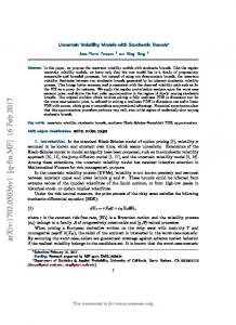
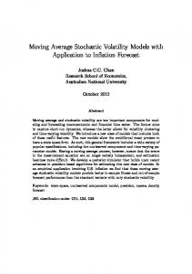
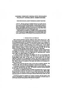
We use the daily returns of CDS index (iTraxx) and TOPIX from 29, Jan., 2007 to 23, May, 2007. The daily returns of them are shown in Fig. 1. [Figure 1 about here.] In the “dual-dynamic-correlation” (DDC) model, the estimates of time-varying correlation, ρ12,t and σ12,t , are shown in Figure 2 [Figure 2 about here.] In the DDC model, the estimates of volatilites, exp(x1,t ) and exp(x2,t ), are shown in Figure 3 [Figure 3 about here.]
7 See 8 The
Kitagawa (1996). justification of an SOSS model is described in Kitagawa (1998).
6
The results of time-varying correlation, ρ12,t and σ12,t , are shown in Fig. 2. These results indicate that the correlations, ρ12,t and σ12,t , change suddenly larger or smaller around 120. The point is the global downturn in stock values, at the end of July, 2007. It indicates that we detect the structural changes in the correlations. We conclude, in financial crises, the correlations of returns and volatilities of financial time series make higher. In the “Single-Dynamic-Correlation-in-Measurement-equation” (SDCM) model, we estimate the model with the dynamic ρ12,t and the invariant σ12 . In Fig. 4, we show the estimates of ρ12,t . [Figure 4 about here.] In the SDCM model, the estimates of volatilities, exp(x1,t ) and exp(x2,t ), are shown in Figure 5 [Figure 5 about here.] In the “Single-Dynamic-Correlation-in-System-equation” (SDCS) model, we estimate the model with the invariant ρ12 and the dynamic σ12,t . In Fig. 6, we show the estimates of σ12,t . [Figure 6 about here.] In the SDCS model, the estimates of volatilities, exp(x1,t ) and exp(x2,t ), are shown in Figure 7 [Figure 7 about here.] We estimate the model with the invariant ρ12 and σ12 . In the “invariant-correlation” (IC) model, the estimates of volatilities, exp(x1,t ) and exp(x2,t ), are shown in Figure 8. [Figure 8 about here.] We compare the log-likelihoods of these models. Table 1 indicates that the log-likelihood of DDC model is largest in the models. [Table 1 about here.]
5
Conclusions
This paper proposes a method to estimate the time-varying interaction of credit and market risks based on the Monte Carlo Particle filter. In this paper, we estimate the time-varying correlation of the returns of credit and market risks and the time-varying correlation of the volatilities of them based on multivariate Stochastic Volatility models withe Dynamic Correlations (MSVDC). The time-varying and invariant parameters in MSVDCs are inferred by the Monte Carlo Particle filter and a self-organizing state space model, proposed by Kitagawa (1996), Gordon et al. (1993), Kitagawa (1998), Yano (2008), and Yano (2007). In our empirical analysis, the time-varying correlations of the return of TOPIX (Tokyo Stock Price Index) and the return of Credit Default Swap (iTraxx) are estimated. We find that the structural changes of the time-varying correlations in the global downturn in stock values, at the end of February, 2007. We conclude, in financial crises, the correlations of returns and volatilities of financial time series make higher. Our findings indicate that any frameworks to estimate the interaction of credit and market risks based on invariant parameters are inadequate. 7
References Alspach, D. L. and H. W. Sorenson (1972). “Nonlinear Bayesian estimation using Gaussian sum approximation”. IEEE Transactions on Automatic Control, 17 pp.439–448. Asai, M., M. McAleer, and J. Yu (2006). “Multivariate Stochastic Volatility: A Review”. Econometric Reviews, 25(2-3) pp.145–175. Breuer, T., M. Jandacka, and G. Krenn (2005). “Towards an Integrated Measurement of Credit Risk and Market Risk”. Proceedings of Banking and Financial Stability: A Workshop on Applied Banking Research. Campbell, J., A. Lo, and C. MacKinlay (1997). The Econometrics of Financial Markets. New Jersey: Princeton University Press. Chib, S., Y. Omori, and M. Asai (2008). “Multivariate Stochastic Volatility”. In T. G. Andersen, R. A. Davis, J. Kreiss, and T. Mikosch, (eds), Handbook of Financial Time Series. New York: Springer-Verlag. in press. A. Doucet, N. de Freitas, and N. Gordon, (eds) (2001). Sequential Monte Carlo Methods in Practice. New York: Springer-Verlag. Gordon, N., D. Salmond, and A. Smith (1993). “Novel approach to nonlinear/non-Gaussian Bayesian state estimation”. IEEE Proceedings-F, 140 pp.107–113. Harvey, A., E. Ruiz, and N. Shephard (1994). “Multivariate Stochastic Variance models”. Review of Economic Studies, 61 pp.247–264. H¨ urseler, M. and H. R. K¨ unsch (2001). “Approximating and maximizing the likelihood for a general state-space model”. In A. Doucet, N. de Freitas, and G. N., (eds), Sequential Monte Carlo Methods in Practice. New York: Springer-Verlag, pp. 159–175. Jazwinski, A. H. (1970). Stochastic Processes and Filtering Theory. New York: Academic Press. Kalman, R. E. (1960). “A new approach to linear filtering and prediction problems”. Transactions of the ASME–Journal of Basic Engineering (Series D), 82 pp.35–45. Kitagawa, G. (1987). “Non-Gaussian State Space Modeling of Nonstationary Time Series”. Journal of the American Statistical Association, 82 pp.1032–1041. Kitagawa, G. (1996). “Monte Carlo filter and smoother for non-Gaussian nonlinear state space models”. Journal of Computational and Graphical Statistics, 5(1) pp.1–25. Kitagawa, G. (1998). “A self-organizing state-space model”. Journal of the American Statistical Association, 93(443) pp.1203–1215. Mandelbrot, B. (1963). “The variation of certain speculative prices”. The Journal of Business, 36 pp.394–419. 8
West, M., P. J. Harrison, and H. S. Migon (1985). “Dynamic generalized linear models and Bayesian forecasting (with discussion)”. Journal of the American Statistical Association, 80 pp.73–97. Yano, K. (2007). “The Monte Carlo particle smoothing and filter initialization based on an inverse system equation”. FSA Discussion Paper Series. No. 2007-1. Yano, K. (2008). “A Self-organizing state space model and simplex initial distribution search”. Computational Statistics, 23 pp.197–216.
9
List of Figures 1 2 3 4 5 6 7 8
The teturns of TOPIX and CDS (iTraxx) [from 2007-Jan-29 DDC model: time-varying correlation (σ12,t and ρ12,t ) . . . DDC model: volatility (exp(x1,t /2) and exp(x2,t /2)) . . . . SDCM model: time-varying correlation (ρ12,t ) . . . . . . . . SDCM model: volatility (exp(x1,t /2) and exp(x2,t /2)) . . . SDCS model: time-varying correlation (σ12,t ) . . . . . . . . SDCS model: volatility (exp(x1,t /2) and exp(x2,t /2)) . . . . IC model: volatility (exp(x1,t /2) and exp(x2,t /2)) . . . . . .
10
to 2007-Aug-31] . . . . . . . . . . . . . . . . . . . . . . . . . . . . . . . . . . . . . . . . . . . . . . . . . . . . . . . . . . . . . . . . . . . . . .
. . . . . . . .
. . . . . . . .
. . . . . . . .
11 12 13 14 15 16 17 18
0 −2 0 −20 −10
iTraxx
10
20 −6
−4
TOPIX
2
Data
0
50
100
150
Time
Figure 1: The teturns of TOPIX and CDS (iTraxx) [from 2007-Jan-29 to 2007-Aug-31]
11
−0.2 −0.6
ρ12,t
0
50
100
150
100
150
0.0 −0.6
σ12,t
0.4
Index
0
50 Index
Figure 2: DDC model: time-varying correlation (σ12,t and ρ12,t )
12
1.6 1.2 0.8
exp(x1,t 2)
0
50
100
150
100
150
150 50 0
exp(x2,t 2)
Index
0
50 Index
Figure 3: DDC model: volatility (exp(x1,t /2) and exp(x2,t /2))
13
0.4 0.2 0.0 −0.6
−0.4
−0.2
ρ12,t
0
50
100
150
Index
Figure 4: SDCM model: time-varying correlation (ρ12,t )
14
1.4 1.1 0.8
exp(x1,t 2)
0
50
100
150
100
150
20 10 0
exp(x2,t 2)
30
Index
0
50 Index
Figure 5: SDCM model: volatility (exp(x1,t /2) and exp(x2,t /2))
15
0.6 0.5 0.4 σ12,t
0.3 0.2 0.1 0.0
0
50
100
150
Index
Figure 6: SDCS model: time-varying correlation (σ12,t )
16
1.6 1.2 0.8
exp(x1,t 2)
0
50
100
150
100
150
60 40 20 0
exp(x2,t 2)
Index
0
50 Index
Figure 7: SDCS model: volatility (exp(x1,t /2) and exp(x2,t /2))
17
1.4 1.2 1.0 0.8
exp(x1,t 2)
0
50
100
150
100
150
10 5 0
exp(x2,t 2)
20
Index
0
50 Index
Figure 8: IC model: volatility (exp(x1,t /2) and exp(x2,t /2))
18
List of Tables 1
Log-likelihood of models . . . . . . . . . . . . . . . . . . . . . . . . . . . . . . . . .
19
20
Table 1: Log-likelihood of models Model DDC Model SDCM Model SDCS Model IC Model
Log-likelihood -368.86 -373.29 -374.32 -379.46
20