Multiview Supervised Dictionary Learning in Speech Emotion

1056

IEEE/ACM TRANSACTIONS ON AUDIO, SPEECH, AND LANGUAGE PROCESSING, VOL. 22, NO. 6, JUNE 2014

Multiview Supervised Dictionary Learning in Speech Emotion Recognition Mehrdad J. Gangeh, Member, IEEE, Pouria Fewzee, Student Member, IEEE, Ali Ghodsi, Mohamed S. Kamel, Life Fellow, IEEE, and Fakhri Karray, Senior Member, IEEE

Abstract—Recently, a supervised dictionary learning (SDL) approach based on the Hilbert-Schmidt independence criterion (HSIC) has been proposed that learns the dictionary and the corresponding sparse coefficients in a space where the dependency between the data and the corresponding labels is maximized. In this paper, two multiview dictionary learning techniques are proposed based on this HSIC-based SDL. While one of these two techniques learns one dictionary and the corresponding coefficients in the space of fused features in all views, the other learns one dictionary in each view and subsequently fuses the sparse coefficients in the spaces of learned dictionaries. The effectiveness of the proposed multiview learning techniques in using the complementary information of single views is demonstrated in the application of speech emotion recognition (SER). The fully-continuous sub-challenge (FCSC) of the AVEC 2012 dataset is used in two different views: baseline and spectral energy distribution (SED) feature sets. Four dimensional affects, i.e., arousal, expectation, power, and valence are predicted using the proposed multiview methods as the continuous response variables. The results are compared with the single views, AVEC 2012 baseline system, and also other supervised and unsupervised multiview learning approaches in the literature. Using correlation coefficient as the performance measure in predicting the continuous dimensional affects, it is shown that the proposed approach achieves the highest performance among the rivals. The relative performance of the two proposed multiview techniques and their relationship are also discussed. Particularly, it is shown that by providing an additional constraint on the dictionary of one of these approaches, it becomes the same as the other. Index Terms—Dictionary learning, emotion recognition, multiview representation, sparse representation, supervised learning.

Manuscript received October 16, 2013; revised February 18, 2014; accepted April 09, 2014. Date of publication April 22, 2014; date of current version May 06, 2014. This work was supported in part by the Natural Sciences and Engineering Research Council (NSERC) of Canada under Canada Graduate Scholarship (CGS D3-378361-2009). The associate editor coordinating the review of this manuscript and approving it for publication was Dr. Dong Yu. M. J. Gangeh was with the Center for Pattern Analysis and Machine Intelligence, Department of Electrical and Computer Engineering, University of Waterloo, Waterloo, ON N2L 3G1, Canada. He is now with the Department of Medical Biophysics, University of Toronto, Toronto, ON M5G 2M9, Canada, and also with the Department of Radiation Oncology, Sunnybrook Health Sciences Center, Toronto, ON M4N 3M5, Canada (e-mail: mehrdad.gangeh@utoronto. ca). P. Fewzee, M. S. Kamel, and F. Karray are with the Center for Pattern Analysis and Machine Intelligence, Department of Electrical and Computer Engineering, University of Waterloo, Waterloo, ON N2L 3G1, Canada (e-mail: [email protected]; [email protected]; [email protected]). A. Ghodsi is with the Department of Statistics and Actuarial Science, University of Waterloo, Waterloo, ON N2L 3G1, Canada (e-mail: [email protected]). Color versions of one or more of the figures in this paper are available online at http://ieeexplore.ieee.org. Digital Object Identifier 10.1109/TASLP.2014.2319157

I. INTRODUCTION HERE are many mathematical models with varying degrees of success to describe data, among which dictionary learning and sparse representation (DLSR) have attracted the interest of many researchers in various fields. Dictionary learning and sparse representation are two closely-related topics that have roots in the decomposition of signals to some predefined bases, such as the Fourier transform. Representation of signals using predefined bases is based on the assumption that these bases are general enough to represent any kind of signal, however, recent research shows that learning the bases1 from data, instead of using off-the-shelf ones, leads to state-of-the-art results in many applications such as texture classification [1]–[3], face recognition [4]–[6], image denoising [7], [8], biomedical tissue characterization [9]–[11], motion and data segmentation [12], [13], data representation and column selection [14], and image super-resolution [15]. In fact, what makes DLSR distinct from the representation using predefined bases is that first, the bases are learned here from the data, and second, only a few components in the dictionary are needed to represent the data (sparse representation). This latter attribute can also be seen in the decomposition of signals using some predefined bases such as wavelets [16]. For a more formal description, let be a finite set of data samples, where is the dimensionality and is the number of data samples. The main goal in classical dictionary learning and sparse representation (DLSR) is to decompose the data over a few dictionary atoms by minimizing a loss function as follows

T

(1) is the dictionary of atoms, and where are the coefficients. The most common loss function in the DLSR literature is the reconstruction error between the original data samples and the decomposed data in the space of the learned dictionary , regularized using a sparsity inducing function to guarantee the sparsity of the coefficients. The most common sparsity inducing function is norm. Hence, (1) can be rewritten as (2) 1Here, the term basis is loosely used as the dictionary can be overcomplete, i.e., the number of dictionary elements can be larger than the dimensionality of the data, and its atoms are not necessarily orthogonal and can be linearly dependent.

2329-9290 © 2014 IEEE. Personal use is permitted, but republication/redistribution requires IEEE permission. See http://www.ieee.org/publications_standards/publications/rights/index.html for more information.

GANGEH et al.: MULTIVIEW SUPERVISED DICTIONARY LEARNING IN SPEECH EMOTION RECOGNITION

where is the th column of . The optimization problem in (2) is mainly based on the minimization of the reconstruction error in mean-squared sense, which is optimal in applications such as denoising, inpainting, and coding [17]. However, the representation obtained from (2) does not necessarily lead to a discriminative representation, which is important in classification tasks. Several approaches have recently been proposed in the literature to include class labels into the optimization problem given in (2) to yield more discriminative representations. These approaches can broadly be grouped into five categories as suggested in [18]2, including: 1) Learning one dictionary per class, where one subdictionary is learned per class and then all these subdictionaries are composed into one. Supervised -means [3], [19], sparse representation-based classification (SRC) [5], metaface [20], and dictionary learning with structured incoherence (DLSI) [21] are in this category. 2) Pruning large dictionaries, in which, initially a very large dictionary is learned in an unsupervised manner, and then the atoms in the dictionary are merged according to some objective function that takes into account the class labels. The supervised dictionary learning approaches based on agglomerative information bottleneck (AIB) [22] and universal visual dictionary [23] are in this category. 3) Learning the dictionary and classifier in one optimization problem, where the optimization problem for the classifier is embedded into the optimization problem given in (2) or its modified version. Discriminative SDL [24] and discriminative K-SVD (DK-SVD) [25] are two techniques in this category. 4) Including class labels in the learning of the dictionary, such as the technique based on information loss minimization (known as info-loss) [26] and the one based on randomized clustering forests (RCF) [27]. 5) Including class labels in the learning of the sparse coefficients or both the dictionary and coefficients such as Fisher discrimination dictionary learning (FDDL) [6]. Recently, a supervised dictionary learning approach has been proposed [18] which is based on the Hilbert Schmidt independence criterion (HSIC) [28], in which the category information is incorporated into the dictionary by learning the dictionary in a space where the dependency between the data and class labels is maximized. The approach has several attractive features such as closed-form formulation for both the dictionary and sparse coefficients, very compact dictionary, i.e., discriminative dictionary at small size, and fast efficient algorithm [18]. Thus, it has been adopted in this paper. There are instances where the data in a dataset is represented in multiple views [29]. This can be due to the availability of several feature sets for the same data such as representation of a document in several languages [30], representation of webpages by both their text and hyperlinks, etc., or due to the availability of information from several modalities, e.g., biometric information for the purpose of authentication that may come from fingerprints, iris, and face. Although single-view representation might be sufficient in a machine learning task for the analysis of the data, complementary information provided by mul2The

interested reader is urged to refer to [18] and the references thereof for a more extensive review on various supervised dictionary learning approaches in the literature and their main advantages and shortcomings.

1057

tiple views usually facilitates the improvement of the learning process. In this paper, we provide the formulation for multiview learning based on the supervised dictionary learning proposed in [18]. Two different methods for multiview representation are proposed and the application to speech emotion recognition using two different feature sets are investigated. Additionally, the multiview approach is extended to continuous labels, i.e., to the case of a regression problem (it was originally proposed for classification tasks using discrete labels [18]). It is worth to note that not all the proposed supervised dictionary learning approaches in the literature can be extended to regression problems. For example, in supervised -means, the discrete labels are needed and it cannot be extended to continuous labels. We will show that the proposed approach can effectively use the complementary information in different feature sets and improve the performance of the recognition system on the AVEC (audio/visual emotion challenge) 2012 emotion recognition dataset compared with some other supervised and unsupervised multiview approaches. The organization of the rest of the paper is as follows: in Section II, the mathematical formulation of the proposed multiview supervised dictionary learning is provided. The application to speech emotion recognition will be discussed in Section III, followed by a discussion of the experimental setup and the results in Section IV. Section V concludes the paper. II. METHODS In this section, the formulation of the proposed multiview supervised dictionary learning (MV-SDL) is provided. To this end, we first briefly review the Hilbert-Schmidt independence criterion (HSIC). Then we provide the formulation for the adopted supervised dictionary learning as being proposed in [18]. Eventually, the mathematical formulation for the proposed MV-SDL is presented. A. Hilbert-Schmidt Independence Criterion HSIC is a kernel-based independence measure between two random variables and [28]. It computes the Hilbert-Schmidt norm of the cross-covariance operators in reproducing kernel Hilbert Spaces (RKHSs) [28], [31]. Suppose that and are two RKHSs in and , respectively. Hence, by the Riesz representation theorem, there are feature mappings and such that and . HSIC can be practically estimated in the RKHSs using a finite number of data samples. Let be independent observations drawn from . The empirical estimate of HSIC can be computed using [28] (3) where

is the trace operator, , and ( is the identity matrix, and is a vector of ones, and hence, is the centering matrix). According to (3), maximizing the

1058

IEEE/ACM TRANSACTIONS ON AUDIO, SPEECH, AND LANGUAGE PROCESSING, VOL. 22, NO. 6, JUNE 2014

empirical estimate of HSIC, i.e., , will lead to the maximization of the dependency between two random variables and .

Algorithm 1 HSIC-Based Supervised Dictionary Learning [18]

B. HSIC-Based Supervised Dictionary Learning

Input: Training data, , test data, , kernel matrix of labels , training data size, , size of dictionary, .

The HSIC-based supervised dictionary learning (SDL) learns the dictionary in a space where the dependency between the data and corresponding class labels is maximized. To this end, it has been proposed in [18] to solve the following optimization problem

Output: Dictionary, data, and .

, coefficients for training and test

1: 2: 3: Compute Dictionary: corresponding to top eigenvalues

s.t.

(4)

where is data samples with the dimensionality of ; is the centering matrix, and its function is to center the data, i.e., to remove the mean from the features; is a kernel on the labels ; and is the transformation that maps the data to the space of maximum dependency with the labels. According to the Rayleigh-Ritz Theorem [32], the solution for the optimization problem given in (4) is the corresponding eigenvectors of the top eigenvalues of . To explain how the optimization problem provided in (4) learns the dictionary in the space of maximum dependency with the labels, using a few manipulations, we note that the objective function given in (4) has the form of empirical HSIC given in (3), i.e.,

(5) where is a linear kernel on the transformed data in the subspace . To derive (5), it is noted that the trace operator is invariant under cyclic permutation, e.g., and also that . Now, it is easy to observe that the form given in (5) is the same as empirical HSIC in (3) up to a constant factor and therefore, it can be easily interpreted as transforming centered data using the transformation to a space where the dependency between the data and class labels is maximized. In other words, the computed transformation constructs the dictionary learned in the space of maximum dependency between the data and class labels. After finding the dictionary , the sparse coefficients can be computed using the formulation given in (2). As explained in [18], (2) can be either solved using iterative methods such as the lasso or in closed-form using soft-thresholding [33], [34] with the soft-thresholding operator , i.e., (6)

eigenvectors of

4: Compute Training Coefficients: For each data sample in the training set, use to compute the corresponding coefficient 5: Compute Test Coefficients: For each data sample in the test set, use to compute the corresponding coefficient where is the th data sample, and are the th elements of and , respectively, and is defined as follows if if otherwise The steps for the computation of the dictionary and coefficients using the HSIC-based SDL is provided in Algorithm 1. The main advantages of the HSIC-based SDL are that the dictionary and coefficients are computed in closed form and separately. Hence, unlike many other SDL techniques in the literature, learning these two do not have to be performed iteratively and alternately. Another remark on the HSIC-based SDL is that unlike many other SDLs in the literature, the labels are not restricted to discrete values and can also be continuous. In other words, the HSIC-based SDL can be easily extended to regression problems, in which the target values are continuous, which is the case in this paper as will be discussed in next sections. C. Multiview Supervised Dictionary Learning In this section, the formulation for two-view supervised dictionary learning is provided; the extension to more than two views is straightforward. The main assumption is that both views agree on the class labels of all instances in the training set. Let and be two views/representations of training samples with the dimensionalities of and , respectively. Having these two representations, the main question is how to perform the learning task using the proposed SDL provided in Algorithm 1. There are two approaches, as follows: Method 1: One approach is to fuse the feature sets from the two views to obtain

, where

. To

GANGEH et al.: MULTIVIEW SUPERVISED DICTIONARY LEARNING IN SPEECH EMOTION RECOGNITION

Algorithm 2 Multiview Supervised Dictionary Learning-Method 1 (MV1)

of

Input: Training data at multiple views, , test data at multiple views, , kernel matrix of labels , training data size, , size of dictionary, . Output: Dictionary, and . data, 1:

.. .

2:

.. .

, coefficients for training and test

Similarly, another subdictionary can be computed by replacing

4: 5: Compute Dictionary: corresponding to top eigenvalues

eigenvectors of

6: Compute Training Coefficients: For each in the fused training set , use data sample to compute the corresponding coefficient 7: Compute Test Coefficients: For each data sample in the fused test set , use to compute the corresponding coefficient learn the supervised dictionary, one needs to use the optimization problem in (4). The columns of , which are the eigenvectors of , construct the dictionary , where is the number of dictionary atoms. Using the formulation given in (2), the sparse coefficients can be subsequently computed for both the training and test sets. These coefficients are submitted to a classifier such as SVM for training or classifying an unknown test sample, respectively. As mentioned in the previous subsection, given the data samples and the dictionary , the formulation given in (2) can be either solved using iterative methods such as the lasso or using a closed-form method such as soft-thresholding given in (6). The latter has the main advantage that it provides the solution in closed form and hence, in lower computation cost compared to iterative approaches like the lasso. Method 2: The alternative approach is to learn one subdictionary from the data samples in each view. In other words, by replacing in (4) we have

s.t.

(7)

By computing the corresponding eigenvectors of the largest , a subdictionary eigenvalues of is obtained, where is the size of the subdictionary for this view.

with the size in (4), i.e.,

s.t.

(8)

and computing the corresponding eigenvectors of the top eigen. By replacing the data values of samples of each view and their corresponding subdictionaries computed in the previous step in the formulation given in (2), the sparse coefficients and can be computed in each view for the training and test samples3. Each of these coefficients can be interpreted as the representation of the data samples in the space of the subdictionary of the corresponding view. These coefficients are then fused such that , where

3:

1059

. Fused coefficients

are

eventually submitted to a classifier such as SVM for training or classifying an unknown test sample. Algorithms 2 and 3 summarize the computation steps for the two multiview approaches proposed in this paper. The connection between the two proposed multiview methods is provided in the Appendix. As proved, by adding an additional constraint on provided in (13) of the appendix, Methods 1 and 2 yield the same results, i.e., the same dictionary and coefficients. This special form of , effectively, decouples the computation of the dictionary and coefficients over two views. In the following sections, the relative performance of these two multiview approaches is shown in the application of emotion recognition. III. SPEECH EMOTION RECOGNITION (SER) Although automatic speech recognition has been around for many years now, it is not always sufficient only to know what is said in a conversation, but sometimes we need to know how something is said. That is due to the fact that a piece of speech can convey much more information than the mere verbal content [35]. Speech emotion recognition attempts to unveil a part of this information, which is related to affection. A natural application of this is to human-computer interaction. That is, to enable computers to adapt to the emotional states of the users, in order to reduce their frustration during interactions [36]. Different modalities (also referred to as social cues) have been used for this purpose, among which only voice cues have led to the discussion of the current section. Given the speech signal , there are two major phases into a solution for speech emotion recognition: 1) extraction of low-level descriptors (LLDs) (acoustic features) from speech, and 2) statistical modeling. Extraction of LLDs is essential, as on the one hand, each speech sample does not convey more than the air pressure recorded by the microphone at a very small fraction of time, therefore one is required to calculate some useful measures of speech that have closer relationship with its affective qualities; on the other hand, speech signals are usually of very high dimensions, hence extracting LLDs also counts as 3The solution can be provided in closed form using (6) as mentioned in Method 1.

1060

IEEE/ACM TRANSACTIONS ON AUDIO, SPEECH, AND LANGUAGE PROCESSING, VOL. 22, NO. 6, JUNE 2014

Algorithm 3 Multiview Supervised Dictionary Learning-Method 2 (MV2) Input: Training data at multiple views, , test data at multiple views, , kernel matrix of labels , training data size, , size of dictionary, . Output: Dictionary, and . data,

, coefficients for training and test

1: 2: for

do

a: b: eigenvalues

eigenvectors of

corresponding to top

c: For each data sample , use corresponding coefficient

in the training set to compute the

d: For each data sample use corresponding coefficient

in the test set , to compute the

3: end for 4: Compute Dictionary:

.. .

.. .

..

.

.. .

.. .

5: Compute Training Coefficients:

6: Compute Test Coefficients:

.. .

a dimensionality reduction stage. Subsequently, at the second stage, given the LLDs, as the covariates (i.e., ), and an affective quality of speech, as the response variable (i.e., in case of discrete affects4, or in case of continuous affects), the idea is to find a mapping between the two: . Later on, this mapping will be used to make predictions on the affective qualities of speech samples. As for the affective qualities, denoted by , two points of view for representing emotional states have been used: categorical and dimensional. According to the categorical view, emotional states [37], [38] can be described using discrete emotion categories such as anger or happiness. On the other hand, a dimensional point of view, also known as the primitive-based point of view, suggests the use of some continuous lower level attributes, e.g., arousal and valence. Theories behind the dimensional representation claim that the space defined by those 4

is the set of nonnegative integers.

dimensions can subsume all the categorical emotional states [39]–[41]. Therefore, depending on the choice of affective qualities, the modeling problem can be recognized as either classification, if the categorical point of view is of interest, or regression, otherwise. Acoustic LLDs are categorized by their domain of extraction. Those which are interpreted in the time and frequency domains are respectively known as prosodic and spectral LLDs. Among prosodic LLDs, pitch, speaking rate, jitter, shimmer, and harmonics-to-noise ratio (HNR) are frequently applied to emotional speech recognition. On the other hand, Mel frequency cepstrum coefficients (MFCC), formant frequencies, energy in different spectral bands (250-650 Hz and 1-4 kHz), and spectral characteristics such as flux, entropy, variance, skewness, and kurtosis, are among the most commonly-used spectral LLDs [42]. A list of about forty LLDs, including prosodic and spectral, has been recently set as a standard [42]–[44], and it appears that the list has been adopted by the research community [45]–[50]. Except for a very few studies [49]–[53], the recent research does not show a major investigation for introduction of new LLDs. On the statistical modeling side, various models and learning algorithms have been used to tackle the problem at hand. Nonetheless, the literature of speech emotion recognition leaves a vast amount of space for experiencing methods based on dictionary learning, particularly those that can incorporate multiple feature sets of different natures, known as multiview dictionary learning. In this work, since we are using two different types of features sets, that is the baseline features of the AVEC 2012, and a set of features that are meant for the analysis of the spectral bands of the speech signal, the multiview dictionary learning approach makes a perfect choice. As for the regression model, we have made use of the lasso, due the sparsity of the linear regression coefficients that it allows, which commonly gives way to a model with better generalization capabilities, and more transparent interpretation of the features space [53]. IV. EXPERIMENTAL RESULTS In this section, first an overview of the emotional speech database used in our experiments is provided, then our choice of acoustic features is described followed by a brief description of some state-of-the-art techniques with which the proposed methods are compared. Eventually, the experiments and the results are presented. A. Dataset Although dozens of emotional speech databases have been collected in the past few years, not all could attract the attention of the research community. SEMAINE, however, has been one of the most well-received databases. A major part of the recent studies on emotional speech recognition [42], [45]–[57] have been conducted relying on the solid-SAL part of the database. Since we have chosen to adopt the database in our experiments, in this subsection, it will be introduced. SEMAINE is recorded using three different sensitive artificial listener (SAL) interaction scenarios [58]: solid SAL, semiautomatic SAL, and automatic SAL. 150 participants (93 female

GANGEH et al.: MULTIVIEW SUPERVISED DICTIONARY LEARNING IN SPEECH EMOTION RECOGNITION

and 57 male) have taken part in the recordings, where their ages range from 22 to 60 ( ). The aim of SAL is to evoke strong emotional responses in a listener by controlling the statements of an operator, i.e., the script is predefined in this scenario. For this purpose, four agents are introduced, and a user can decide which operator to talk to at any time. Each of those agents tries to simulate one of four different emotions: happiness, sadness, anger, and sensibility. Solid SAL [59], [60], on the other hand, is a similar scenario to SAL, for which there is no predefined script given to the operators. Instead, they are free to act as one of the four SAL agents at any time. This is done for the sake of a more natural face-to-face conversation. Despite the relatively young age of the database, it has been a target of various studies already. The main reasons for the attraction towards the SEMAINE are first [42] and second [61] audio/ visual emotion challenge (AVEC), which have set the solid SAL part of the database as the benchmark. For the sake of these challenges, four dimensions were used: arousal, expectation, power, and valence. Our study is conducted based on the fully-continuous sub-challenge (FCSC) of the AVEC 2012. For the FCSC, the features are extracted at 0.5 second intervals, considering only the spoken parts of the recordings [61]. To extract features from the spoken parts of the speech signal, we have used the same timing as provided by the baseline features. In other words, each instant in the SED features vector corresponds to an instant in the baseline feature vector, where the two are extracted from the same window. According to the settings of this challenge, three subsets of the database were used for the training, development, and testing purposes. Since the labels of the test subset were not released to the public, our experiments are performed based on the other two subsets. That is to say, for each experiment, a model is trained using the training set, and it is evaluated using the development set. To be more specific, all training and tuning the parameters are performed on the training set, during which the development set is remained unseen. The performance of the systems is eventually evaluated on the development set, which serves as the test set in the experiments. The number of samples in the training and development sets are 10806 and 9312, respectively. This number of samples comes from 31 and 32 different interaction sessions, for training and developments sets, respectively.

B. Audio Features Different acoustic low-level descriptors (LLDs), also referred to as low-level descriptors, have been employed for the emotional recognition of speech. In the following, a review of the spectral energy distribution is provided, followed by a brief introduction of the baseline features of the AVEC 2012 [61]. In the previous works [53], [62], we have observed the efficiency of the spectral energy distribution as a set of features for analyzing emotional speech, in this work we have decided to combine those with the prevalently used set of features. Farther in this study, we show how the addition of this set of features improves the prediction accuracy of the overall model. 1) Spectral energy distribution (SED): Spectral energy distribution (SED) is comprised of a set of components, where each

1061

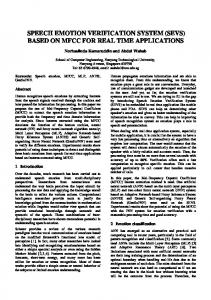
Fig. 1. (a) A speech signal (b) SED component for , and (c) SED com, where is the normalizing factor as introduced in (10). ponent for

component represents the relative energy of the signal in a spe, cific band of the spectrum [53], [62]. For a speech signal the definition of the component is as follows.

(9) is the discrete Fourier transform of ; is the where and unit step function (a.k.a. the Heaviside step function); indicate the lower and upper bounds of the component in the is a normalizing function, the use of which spectrum; and is discussed in the remainder of this section. In this equation, denotes the number of samples of the signal, which by principle equals the length of the signal times its sampling frequency. Fig. 1(a) and 1(b) show an arbitrary speech signal and the SED components of the signal, respectively. In Fig. 1(b), the is assumed to be the identity function, normalizing function therefore the SED components form a binned power spectrum of the speech signal. Regardless of how informative each of the components is, they can take arbitrarily large or small values. In other words, although some intervals appear to carry a relatively minor part of the energy of the signal, they can play a role as important as that of the others, if not more so. Therefore, as a natural solution, we normalize the Fourier transform of the signal over the in the definition of spectrum by incorporating the function the SED: (10) is because The reason why is set to take values from we normalize the amplitude of the speech signal to take values between zero and one; since this property will be preserved by the discrete Fourier transform, raising to the power of inflates

1062

IEEE/ACM TRANSACTIONS ON AUDIO, SPEECH, AND LANGUAGE PROCESSING, VOL. 22, NO. 6, JUNE 2014

. Fig. 1(c) shows the effect of this normalization on SED components. This is similar to the idea of log spectrum, however, this provides a degree of freedom, i.e., , that could be set through cross-validation, given the problem of interest. As for the parameter setting of SED, except the maximum value of the higher bound on the spectrum, which is dictated by the sampling frequency (Nyquist theorem), the length of each interval and the power have to be set according to the modeling criteria. For the purpose of our experiments, extraction of SED components is done from non-overlapping 100 ms windows of speech signal. The spectral interval length is set to 100 Hz. They cover from 0 to 8 kHz. The value of is selected as 0.2. These parameters are all chosen based on a line search. The min, max, median, mean, and standard deviation of the features are used as the statistics computed over the windows of the speech signal. The dimensionality of this SED feature set is 400. 2) AVEC 2012 audio baseline features: The baseline features provided by the AVEC 2012 [61] have the dimensionality of 1841, consisting of 25 energy and spectral-related functionals, 6 voice-related functionals, 25 delta functionals, and 10 coefficients of the voice-related voiced/unvoiced durational features. The details of the features and functionals are provided in [61, Tables 4 and 5]. C. Comparison to the State of the Art In this subsection, the explanation is provided for four approaches in the literature, with which our results are compared. These four approaches are two from dictionary learning and sparse representation literature, one from a recently published paper in multiview emotion recognition, and the AVEC 2012 baseline system [61] as described in the following paragraphs. 1) Unsupervised k-means: Although -means is known as a clustering approach and hence, an unsupervised technique, in dictionary learning and sparse representation (DLSR) literature, it has been used in both unsupervised and supervised paradigms [18], [19]. In this context, if -means is applied to all training samples on all classes, it is considered as an unsupervised dictionary. However, if the cluster centers are computed on the training samples of each class using -means separately, eventually composed into one dictionary, the dictionary obtained is supervised, and the approach is called supervised -means, which is belonging to one dictionary per class category of SDL approaches mentioned in Section I. Supervised -means is designed for discrete labels and it cannot be extended to continuous labels which is the case in speech emotion recognition application using dimensional affects. Hence, here, unsupervised -means has been used as one of the dictionary learning approaches to be compared with the proposed approach. For multiview learning using -means, the feature sets are first fused and then submitted to the -means for computing the dictionary. The sparse coefficients are learned using (2). Since the dictionary is not orthogonal in this case, unlike the proposed approach, (2) can be only computed using iterative approaches and it does not have closed-form solution. 2) Discriminative K-SVD: To provide a comparison with the supervised dictionary learning (SDL) approaches in the

literature, as mentioned in Section I, not all the proposed SDL methods in the literature are extendible to continuous labels. For example, all of the SDL methods in category 1 mentioned in Section I, i.e., one dictionary per class category, need discrete class labels and none of them can be applied to continuous labels. Among the SDL approaches in the literature, we have chosen the discriminative K-SVD (DK-SVD) [25] approach that jointly learns the dictionary and a linear classifier in one optimization problem. Although DK-SVD was originally proposed for classification problem, i.e., for discrete labels, it can be easily extended to regression problems (for continuous labels). It is sufficient to replace the discrete labels in the formulation provided in [25] with continuous labels, all other steps remain unchanged. To implement multiview DK-SVD, the same as multiview -means, the features from single views are fused and then submitted to the DK-SVD formulation provided in [25]. 3) Cross-Modal Factor Analysis (CFA): The proposed multiview SDL approach in this paper is a supervised multiview technique as the class labels are included in the learning process. There are, however, unsupervised approaches in the literature that perform multiview analysis by including the correlation among the views into the learning process without taking into account the class labels. Cross-modal factor analysis (CFA) [63] is one of these approaches, which has recently been introduced in the context of multiview emotion recognition [64]. CFA is an unsupervised approach that includes the relationship between the two views by minimizing the norm distance between the projected points into two orthogonal subspaces. Subsequently, the projected data points into the coupled subspaces are computed and concatenated to jointly represent the data. They are eventually submitted to a regressor for its training using the training set, and subsequently predicting the dimension of an unknown emotion. Unlike other approaches discussed in this paper, CFA does not lead to a sparse representation. 4) AVEC 2012 Baseline System: The AVEC 2012 baseline system [61] is comprising of baseline features submitted to support vector machines regression (SVR). Here, the original baseline feature set is used with a dimensionality of 1841 features, whereas in previous three approaches, the dimensionality is determined by the dictionary size (in unsupervised -means and DK-SVD) or the number of components in the jointly learned subspaces (in CFA), which is far less than the original feature set size in our experiments (maximum 64).

D. Implementation Details Two feature sets described above have been used, i.e., SED and baseline features, as the two views and for a speech emotion recognition (SER) system based on the multiview SDL proposed earlier in this paper. Hence, the two views are and , where is 10806 in the training set (which is used for both training and tuning the parameters) and 9312 in the development set (which serves as the test set) for the FCSC part of the dataset in the experiments. There are four dimensional affects, i.e., arousal (A), expectation (E), power (P), and Valance (V), as the continuous response variables to be predicted. Hence, a regressor is to be deployed in the SER system. The lasso regressor and its

GANGEH et al.: MULTIVIEW SUPERVISED DICTIONARY LEARNING IN SPEECH EMOTION RECOGNITION

1063

Fig. 2. The percentage of correlation coefficient ( ) of the speech expression recognition (SER) systems based on single-view (SV) and multiview (MV) learning approaches. MV1 and MV2 are the multiview SDL techniques based on Algorithms 2 and 3, respectively as discussed in Section II-C. The results are shown at four different dictionary sizes for (a) arousal, (b) expectation, (c) power, (d) valence, and (e) average over all dimensional affects.

GLMNET5 implementation are used in all approaches except for DK-SVD that learns its own linear regressor and AVEC 2012 baseline system that deploys a SVR. The sparsity parameter of the lasso regressor has been optimized over the training set by a 10-fold cross validation. As for the SVR, a linear-kernel is used in the experiments and the trade-off parameter ( ) of the SVR is tuned by a line search over the , and by 5-fold set of values of cross validation on the training set. An RBF kernel is used over 5http://www-stat.stanford.edu/tibs/glmnet-matlab/.

the response variable in each dimension, which serves as the kernel over the target values ( ) to compute in Algorithms 2 and 3. The kernel width of the RBF kernel has been set by using a self-tuning approach similar to what is explained in , which is the average [65], i.e., (Euclidean) distance between a response variable and all others. The training set is used to compute the dictionary. The optimal value of the regularization parameter in soft thresholding ( ) for the proposed multiview dictionary learning methods, which controls the level of sparsity, has been computed by 10-fold

1064

IEEE/ACM TRANSACTIONS ON AUDIO, SPEECH, AND LANGUAGE PROCESSING, VOL. 22, NO. 6, JUNE 2014

cross-validation on the training set. The is then used to compute the coefficients for both training and test sets6. In all experiments, the data in each view is normalized such that each feature is mapped to the range of [0,1]. As suggested in [61], the performance of the SER system is evaluated using Pearson’s correlation coefficient ( ) for each session:

TABLE I THE AVERAGE LEARNING TIME (INCLUDING THE TIME REQUIRED FOR LEARNING THE DICTIONARY AND THE COEFFICIENTS, TUNING THE SPARSITY PARAMETER FOR THE LASSO REGRESSOR, AND EVENTUALLY TRAINING THE REGRESSOR USING TUNED PARAMETERS) AND RECALL TIME (BOTH IN SECONDS) FOR THE SINGLE-VIEW AND MULTIVIEW SER SYSTEMS. THE COMPUTATION TIME IS AVERAGED OVER ALL THE DIMENSIONAL AFFECTS FOR EACH METHOD. THE RESULTS ARE REPORTED FOR FOUR DICTIONARY SIZES 8, 16, 32, AND 64

(11) where, is the total number of data samples in a session; and represent the actual and predicted dimensional affects and are the means of those in a session, respectively; values. The correlation between the predicted and actual values is calculated for each session according to (11). However, since sessions are of different lengths, the contribution of each session in the total correlation should be different. Therefore, to calculate the overall correlation coefficient ( ), we have used the weighted average of session correlations, where sessions’ lengths are used as for the weights: (12) is the total length of sessions (which is equivalent to where and are the length and the total number of data samples), the correlation coefficient of session , respectively, and is the total number of sessions. E. Results and Discussions The correlation coefficients ( ) for HSIC-based SDL at single view (Algorithm 1) and also for the proposed multiview SER systems (Algorithms 2 and 3) and rival multiview approaches computed over the two feature sets, i.e., SED and baseline features, are reported in Fig. 2 for the arousal, expectation, power, and valence dimensions at four dictionary sizes, i.e., 8, 16, 32, and 64. The average over all four dimensions of learning time (including the time required to learn the dictionary and coefficients, the tuning time for the sparsity coefficient of the regressor, and also the time for training the regressor) as well as recall (test) time are provided in Table I. Since there is no dictionary associated with the AVEC 2012 baseline system, the results related to this approach are separately provided in Table II. The values for the statistical test of significance (paired -test) performed pairwise between the proposed multiview approaches and all single view or rival approaches are reported in Table III. As can be seen in Fig. 2, both proposed multiview approaches (MV1 and MV2) benefit from the complementary information in two-view features sets. The performance of the single-view system based on the SED is usually inferior to the one based on the baseline feature set. However, combining these two representations using one of the proposed multiview approaches discussed earlier leads to higher correlation coefficients in all dimensions (except for MV1 in expectation dimension). The results of statistical significance test (Table III) show that both 6One is computed for each data point in the training set. However, the over the whole training set is used to compute the coefficients on averaged the training and test sets as it yields better generalization.

MV1 and MV2 significantly outperform ( ) single view method based on SED features. Moreover, MV2 significantly outperforms the other single view method, which is using baseline features. For the purpose of comparing the proposed multiview SDL methods with the AVEC 2012 baseline system, if we take the average of correlation coefficient over all dimensions and dictionary sizes, MV1 and MV2 achieve an average performance of 15.27% and 16.17%, respectively, whereas the average correlation coefficient over all four dimensions for the AVEC 2012 baseline system is 14.8%, which is less than (although not significant according to Table III) the performance of the proposed methods. Also, since original baseline features, i.e., 1841 features, are used in the AVEC 2012 baseline system, the dimensionality is much higher than the dictionary learning approaches (maximum 64). Consequently, the computational time for both learning and recalling are much longer than all other approaches. For example, the average recall time over all dimensions for the AVEC 2012 baseline system (665 s) is more than 10000 times longer than the same for the proposed MV1 (0.057) and MV2 (0.062 s). Furthermore, the proposed MV2 significantly (see Table III) outperforms other multiview approaches in the literature. Also, the performance of the proposed MV1 is significantly better than MV DK-SVD. Supervised multiview methods, i.e., multiview DK-SVD, MV1, and MV2 particularly benefit from the information in target values’ information (dimensional affects) at small dictionary size as can be observed from the results at the dictionary size of 8 in Fig. 2. For example, for power dimensional affect, MV1 performs about twice as good as the unsupervised multiview techniques, i.e., -means and CFA. By increasing the dictionary size, however, the unsupervised multiview approaches can capture the underlying correlation among the single view feature sets, hence their performance approaches those of the supervised multiview techniques. Nevertheless, the main advantage of better performance at small dictionary sizes is much lower computational cost, as increasing the number of

GANGEH et al.: MULTIVIEW SUPERVISED DICTIONARY LEARNING IN SPEECH EMOTION RECOGNITION

1065

TABLE II THE PERCENTAGE OF CORRELATION COEFFICIENT ( ), LEARNING, AND RECALL TIME (IN SECONDS) FOR THE AVEC 2012 BASELINE SYSTEM USING THE BASELINE FEATURES AND A SUPPORT VECTOR MACHINE REGRESSION (SVR) WITH LINEAR KERNEL

TESTS

TABLE III STATISTICAL SIGNIFICANCE (PAIRED -Test) BETWEEN PROPOSED MULTIVIEW METHODS (MV1 OR MV2) AND SINGLE VIEW OR RIVAL MULTIVIEW APPROACHES. -VALUES ARE SHOWN FOR THE PROPOSED MV METHODS VS. THE SINGLE VIEW OR RIVAL APPROACH

OF

dictionary atoms also increases the computational time. On the other hand, between the two supervised approaches, while the proposed multiview approaches provide a closed-form solution for both the dictionary and coefficients, multiview DK-SVD optimization problem is nonconvex and the solution has to be performed iteratively and alternately for the dictionary and coefficients [25] using an iterative algorithm such as K-SVD [66]. This has two main disadvantages, first, it increases the computation time, and second, the algorithm may get stock in a local minimum solution. The latter disadvantage of DK-SVD algorithm explains its poor performance in expectation dimension for the dictionary sizes of 16, 32, and 64. Moreover, in average, the performance of DK-SVD is far behind the proposed MV1 and MV2. Not to mention that it is learning time is the longest after AVEC 2012 baseline system, as tuning its parameters is very time consuming, and makes this approach unsuitable in the applications where online learning is required. In terms of the complexity of methods, the proposed multiview approaches are the least complex as their solution is closed form for both the dictionary and coefficients. Although learning the dictionary and coefficients does not have to be done iteratively and alternately for the MV -means method, neither the dictionary nor the coefficients can be learned in closed form, which makes both learning and recalling time for this method relatively long (see Table I). As can be seen in Table I, the proposed MV1 and MV2 are computationally much more efficient than the other two dictionary-based multiview approaches, i.e., -means and DK-SVD. Although CFA also offers a closed-form solution using singular value decomposition, unlike MV1 and MV2, it does not lead to a sparse representation in the subspaces. Both CFA and proposed multiview approaches can be kernelized. The formulation for the kernelized CFA has been provided in [64]. A kernelized version of HSIC-based SDL was proposed in [18]. The extension to multiview learning is straightforward and leads to similar algorithms as in Algorithms 2 and 3. However, the kernelized version of the proposed multiview approach will lead to a sparse representation, which is an advantage for the approach compared to the kernelized CFA. The proposed MV1 and MV2 approaches can be easily extended to more than two views as shown in Algorithms 2 and 3. This is not the case for the extension of the CFA to more than two views as the correlation between every two views has to be computed pairwise

using an optimization problem given in [64]. However, this may not lead to unique solutions for the subspaces. Considering that MV1 and MV2 achieve an average correlation coefficient over all dictionary sizes and dimensions of 15.27% and 16.17%, respectively reveals higher performance of MV2 compared to MV1 in average. If we also take into account the computation time, that is learning time for MV2 is faster than MV1, MV2 seems to be the more favorable of the two. As a final remark, it is worth to mention that MV2 learns the dictionary and coefficients in the two views independently, and only fuses the features in the space of leaned dictionaries at the final stage. This is expected to be useful when the two views are independent or not very much correlated. If this is not the case, learning the dictionary in a fused space of two views might be beneficial, as the dictionary learned can share the common properties of both views. This can be especially useful for small dictionary sizes. V. CONCLUSION In this paper, a multiview supervised dictionary learning was proposed for multiview representation analysis of speech emotion recognition. Two different multiview methods were proposed: fusing the feature sets in the original space, and learning one dictionary and corresponding coefficients in this fused space (MV1), or learning one dictionary and the corresponding coefficients in each view, and then fusing the representations in the learned dictionary spaces (MV2). It is shown that both methods benefit from the complementary information in multiple views. However, MV2 learns in the space of each view independently from others, whereas MV1 learns in the space of all views simultaneously. The relative performance of the two proposed multiview SDL approaches was demonstrated in speech emotion recognition (SER). In average, it was shown that MV2 outperforms the MV1 method. However, both proposed multiview approaches could capture the complementary information in both views to improve the performance over single views. In terms of computational cost, the learning time for the MV2 is shorter than the same for MV1 in SER application. But their average recall time is almost the same. The MV2 also provides one additional parameter to tune, which is the relative dictionary sizes

1066

IEEE/ACM TRANSACTIONS ON AUDIO, SPEECH, AND LANGUAGE PROCESSING, VOL. 22, NO. 6, JUNE 2014

in multiple views. This additional parameter gives higher flexibility to this approach as it can be tuned over the training set to achieve higher performance. To avoid spending too much time on tuning this parameter, the relative size of the dictionaries in multiple views can be selected based on the relative performance of their corresponding single views, and assigning more dictionary atoms to those views with higher performance in the single view. APPENDIX A CONNECTION BETWEEN TWO PROPOSED MULTIVIEW METHODS The approach provided in Method 2 can be considered as a special case of Method 1. To better realize how these two approaches are related, in Method 1 can be considered to be of the special form as follows (13) Considering this form of , it is easy to show: 1) The constraint given in (4) is equivalent to two constraints given in (7) and (8):

(14) where is a identity matrix and . From the last equality in (14), it is easy to conclude the constraints given in (7) and (8), i.e., and , where the dimensionality of the identity matrices is explicitly shown in the subscripts to prevent confusion. Consequently, this means that the dictionaries learned by the two methods are the same for the special form of given in (13). 2) The coefficients obtained from Method 1 will also be equivalent to the coefficients

computed

using Method 2. This can be shown by using the formulation given in (2), the special form of given in (13), and by recalling that

as follows7,8:

(15) The bottom line of (15) is effectively consisting of two formulations, i.e., for view and for view . This shows that for the special form of given in (13), 7

is used instead of

in (2) as the dictionary elements are the columns of

. 8Here, -norm is used over a matrix, and it is meant that -norms over each column of the matrix are summed such as what is used in (2).

the coefficients computed using Method 1 are the same as those computed using Method 2. In summary, it can be concluded that by adding an additional constraint on as provided in (13), Methods 1 and 2 yield the same results, i.e., the same dictionary and coefficients. This special form, effectively, decouples the computation of the dictionary and coefficients over two views. REFERENCES [1] M. J. Gangeh, A. Ghodsi, and M. S. Kamel, “Dictionary learning in texture classification,” in Proc. 8th Int. Conf. Image Analysis and Recognition - Volume Part I. Berlin, Heidelberg, Germany: Springer-Verlag, 2011, pp. 335–343. [2] J. Xie, L. Zhang, J. You, and D. Zhang, “Texture classification via patch-based sparse texton learning,” in Proc. 17th IEEE Int. Conf. Image Process. (ICIP), 2010, pp. 2737–2740. [3] M. Varma and A. Zisserman, “A statistical approach to material classification using image patch exemplars,” IEEE Trans. Pattern Anal. Mach. Intell., vol. 31, no. 11, pp. 2032–2047, Nov. 2009. [4] C. Zhong, Z. Sun, and T. Tan, “Robust 3D face recognition using learned visual codebook,” in Proc. IEEE Conf. Comput. Vis. Pattern Recogn. (CVPR), 2007, pp. 1–6. [5] J. Wright, A. Yang, A. Ganesh, S. Sastry, and Y. Ma, “Robust face recognition via sparse representation,” IEEE Trans. Pattern Anal. Mach. Intell., vol. 31, no. 2, pp. 210–227, Feb. 2009. [6] M. Yang, L. Zhang, X. Feng, and D. Zhang, “Fisher discrimination dictionary learning for sparse representation,” in Proc. 13th IEEE Int. Conf. Comput. Vis. (ICCV), 2011, pp. 543–550. [7] M. Elad and M. Aharon, “Image denoising via sparse and redundant representations over learned dictionaries,” IEEE Trans. Image Process., vol. 15, no. 12, pp. 3736–3745, Dec. 2006. [8] J. Mairal, M. Elad, and G. Sapiro, “Sparse representation for color image restoration,” IEEE Trans. Image Process., vol. 17, no. 1, pp. 53–69, Jan. 2008. [9] M. J. Gangeh, L. Sørensen, S. B. Shaker, M. S. Kamel, M. de Bruijne, and M. Loog, “A texton-based approach for the classification of lung parenchyma in CT images,” in Proc. Int. Conf. Med. Image Comput. Comput. Assisted Intervent. (MICCAI). Berlin, Heidelberg, Germany: Springer-Verlag, 2010, pp. 595–602. [10] L. Sørensen, M. J. Gangeh, S. B. Shaker, and M. de Bruijne, “Texture classification in pulmonary CT,” in Lung Imaging and Computer Aided Diagnosis, A. El-Baz and J. S. Sure, Eds. Boca Raton, FL, USA: CRC, 2007, pp. 343–367. [11] M. J. Gangeh, A. Sadeghi-Naini, M. S. Kamel, and G. Czarnota, “Assessment of cancer therapy effects using texton-based characterization of quantitative ultrasound parametric images,” in Proc. Int. Symp. Biomed. Imaging: From Nano to Macro (ISBI), 2013, pp. 1360–1363. [12] S. Rao, R. Tron, R. Vidal, and Y. Ma, “Motion segmentation via robust subspace separation in the presence of outlying, incomplete, or corrupted trajectories,” in Proc. IEEE Conf. Comput. Vis. Pattern Recognit. (CVPR), 2008, pp. 1–8. [13] E. Elhamifar and R. Vidal, “Sparse subspace clustering,” in IEEE Conf. Comput. Vis. Pattern Recognit. (CVPR), 2009, pp. 2790–2797. [14] E. Elhamifar, G. Sapiro, and R. Vidal, “See all by looking at a few: Sparse modeling for finding representative objects,” in Proc. IEEE Conf. Comput. Vis. Pattern Recognit. (CVPR), 2012, pp. 1600–1607. [15] J. Yang, J. Wright, T. Huang, and Y. Ma, “Image super-resolution via sparse representation,” IEEE Trans. Image Process., vol. 19, no. 11, pp. 2861–2873, Nov. 2010. [16] S. Mallat, A Wavelet Tour of signal Processing: The Sparse Way, 3rd ed. ed. New York, NY, USA: Academic, 2009. [17] K. Huang and S. Aviyente, “Sparse representation for signal classification,” in Advances in Neural Information Processing Systems (NIPS). Cambridge, MA, USA: MIT Press, 2007, pp. 609–616. [18] M. J. Gangeh, A. Ghodsi, and M. S. Kamel, “Kernelized supervised dictionary learning,” IEEE Trans. Signal Process., vol. 61, no. 19, pp. 4753–4767, Oct. 2013. [19] M. Varma and A. Zisserman, “A statistical approach to texture classification from single images,” Int. J. Comput. Vis.: Special Issue Texture Anal Synth., vol. 62, no. 1-2, pp. 61–81, 2005. [20] M. Yang, L. Zhang, J. Yang, and D. Zhang, “Metaface learning for sparse representation based face recognition,” in Proc. 17th IEEE Int. Conf. Image Process. (ICIP), 2010, pp. 1601–1604.

GANGEH et al.: MULTIVIEW SUPERVISED DICTIONARY LEARNING IN SPEECH EMOTION RECOGNITION

[21] I. Ramirez, P. Sprechmann, and G. Sapiro, “Classification and clustering via dictionary learning with structured incoherence and shared features,” in Proc. IEEE Conf. Comput. Vis. Pattern Recognit. (CVPR), 2010, pp. 3501–3508. [22] B. Fulkerson, A. Vedaldi, and S. Soatto, “Localizing objects with smart dictionaries,” in Proc. 10th Eur. Conf. Comput. Vis. (ECCV): Part I, 2008, pp. 179–192. [23] J. Winn, A. Criminisi, and T. Minka, “Object categorization by learned universal visual dictionary,” in Proc. 10th IEEE Int. Conf. Computer Vision (ICCV), 2005, pp. 1800–1807. [24] J. Mairal, F. Bach, J. Ponce, G. Sapiro, and A. Zisserman, “Supervised dictionary learning,” in Advances in Neural Information Processing Systems (NIPS). Cambridge, MA, USA: MIT Press, 2008, pp. 1033–1040. [25] Q. Zhang and B. Li, “Discriminative K-SVD for dictionary learning in face recognition,” in Proc. IEEE Conf. Comput. Vis. Pattern Recognit. (CVPR), 2010, pp. 2691–2698. [26] S. Lazebnik and M. Raginsky, “Supervised learning of quantizer codebooks by information loss minimization,” IEEE Trans. Pattern Anal. Mach. Intell., vol. 31, no. 7, pp. 1294–1309, Jul. 2009. [27] F. Moosmann, B. Triggs, and F. Jurie, “Fast discriminative visual codebooks using randomized clustering forests,” in Advances in Neural Information Processing Systems (NIPS). Cambridge, MA, USA: MIT Press, 2006, pp. 985–992. [28] A. Gretton, O. Bousquet, A. Smola, and B. Schölkopf, “Measuring statistical dependence with Hilbert-Schmidt norms,” in Proc. 16th Int. Conf. Algorithmic Learn. Theory (ALT), 2005, pp. 63–77. [29] A. Blum and T. Mitchell, “Combining labeled and unlabeled data with co-training,” in Proc. 11th Annu. Conf. Comput. Learn. Theory, 1998, pp. 92–100. [30] M. R. Amini, N. Usunier, and C. Goutte, “Learning from multiple partially observed views - an application to multilingual text categorization,” in Advances in Neural Information Processing Systems (NIPS). Cambridge, MA, USA: MIT Press, 2009, pp. 28–36. [31] N. Aronszajn, “Theory of reproducing kernels,” Trans. Amer. Math. Soc., vol. 68, no. 3, pp. 337–404, 1950. [32] H. Lütkepohl, Handbook of Matrices. New York, NY, USA: Wiley, 1996. [33] D. L. Donoho and I. M. Johnstone, “Adapting to unknown smoothness via wavelet shrinkage,” J. Amer. Statist. Assoc., vol. 90, no. 432, pp. 1200–1224, 1995. [34] J. Friedman, T. Hastie, H. Hofling, and R. Tibshirani, “Pathwise coordinate optimization,” Ann. Appl. Statist., vol. 1, no. 2, pp. 302–332, 2007. [35] C. Caffi and R. W. Janney, “Toward a pragmatics of emotive communication,” J. Pragmatics, vol. 22, no. 3-4, pp. 325–373, 1994. [36] R. W. Picard, “Affective computing for HCI,” Human-Comput. Interact.: Ergonom. User Interfaces, vol. 1, pp. 829–833, 1999. [37] P. Ekman, Basic Emotions. Sussex, U.K.: Wiley, 1999. [38] R. Cowie, E. Douglas-Cowie, N. Tsapatsoulis, G. Votsis, S. Kollias, W. Fellenz, and J. Taylor, “Emotion recognition in human-computer interaction,” IEEE Signal Process. Mag., vol. 18, no. 1, pp. 32–80, Jan. 2001. [39] J. A. Russell, “A circumplex model of affect,” J. Personal. Social Psychol., vol. 39, pp. 1161–1178, 1980. [40] A. Mehrabian, “Pleasure-arousal-dominance: A general framework for describing and measuring individual differences in temperament,” Current Psychol., vol. 14, pp. 261–292, 1996. [41] J. Fontaine, K. Scherber, E. Roesch, and P. Ellsworth, “The world of emotions is not two-dimensional,” Psychol.Sci., vol. 18, no. 12, pp. 1050–1057, 2007. [42] B. Schuller, M. Valstar, F. Eyben, G. McKeown, R. Cowie, and M. Pantic, “AVEC 2011–the first international audio/visual emotion challenge,” in Affective Computing and Intelligent Interaction, ser. Lecture Notes in Computer Science. Berlin/Heidelberg, Germany: Springer, 2011, vol. 6975, pp. 415–424. [43] B. Schuller, S. Steidl, and A. Batliner, “The Interspeech 2009 emotion challenge,” in Proc. Interspeech, 2009, pp. 312–315. [44] B. Schuller, S. Steidl, A. Batliner, F. Burkhardt, L. Devillers, C. Müller, and S. S. Narayanan, “The Interspeech 2010 paralinguistic challenge,” in Proc. Interspeech, 2010, pp. 2794–2797. [45] R. Calix, M. Khazaeli, L. Javadpour, and G. Knapp, “Dimensionality reduction and classification analysis on the audio section of the semaine database,” in Affective Computing and Intelligent Interaction, ser. Lecture Notes in Computer Science. Berlin/Heidelberg, Germany: Springer, 2011, vol. 6975, pp. 323–331.

1067

[46] L. Cen, Z. Yu, and M. Dong, “Speech emotion recognition system based on L1 regularized linear regression and decision fusion,” in Affective Computing and Intelligent Interaction, ser. Lecture Notes in Computer Science. Berlin/Heidelberg, Germany: Springer, 2011, vol. 6975, pp. 332–340. [47] S. Pan, J. Tao, and Y. Li, “The CASIA audio emotion recognition method for audio/visual emotion challenge 2011,” in Affective Computing and Intelligent Interaction, ser. Lecture Notes in Computer Science. Berlin/Heidelberg, Germany: Springer, 2011, vol. 6975, pp. 388–395. [48] G. Ramirez, T. Baltrušaitis, and L.-P. Morency, “Modeling latent discriminative dynamic of multi-dimensional affective signals,” in Affective Computing and Intelligent Interaction, ser. Lecture Notes in Computer Science. Berlin/Heidelberg, Germany: Springer, 2011, vol. 6975, pp. 396–406. [49] A. Sayedelahl, P. Fewzee, M. Kamel, and F. Karray, “Audio-based emotion recognition from natural conversations based on co-occurrence matrix and frequency domain energy distribution features,” in Affective Computing and Intelligent Interaction, ser. Lecture Notes in Computer Science. Berlin/Heidelberg, Germany: Springer, 2011, vol. 6975, pp. 407–414. [50] R. Sun and E. Moore, “Investigating glottal parameters and teager energy operators in emotion recognition,” in Affective Computing and Intelligent Interaction, ser. Lecture Notes in Computer Science, S. D’Mello, A. Graesser, B. Schuller, and J.-C. Martin, Eds. Berlin/Heidelberg, Germany: Springer, 2011, vol. 6975, pp. 425–434. [51] J. Kim, H. Rao, and M. Clements, “Investigating the use of formant based features for detection of affective dimensions in speech,” in Affective Computing and Intelligent Interaction, ser. Lecture Notes in Computer Science. Berlin/Heidelberg, Germany: Springer, 2011, vol. 6975, pp. 369–377. [52] H. Meng and N. Bianchi-Berthouze, “Naturalistic affective expression classification by a multi-stage approach based on hidden markov models,” in Affective Computing and Intelligent Interaction, ser. Lecture Notes in Computer Science. Berlin/Heidelberg, Germany: Springer, 2011, vol. 6975, pp. 378–387. [53] P. Fewzee and F. Karray, “Elastic net for paralinguistic speech recognition,” in Proc. 14th ACM Int. Conf. Multimodal Interact., 2012, pp. 509–516. [54] A. Cruz, B. Bhanu, and S. Yang, “A psychologically-inspired match-score fusion model for video-based facial expression recognition,” in Affective Computing and Intelligent Interaction, ser. Lecture Notes in Computer Science. Berlin/Heidelberg, Germany: Springer, 2011, vol. 6975, pp. 341–350. [55] M. Dahmane and J. Meunier, “Continuous emotion recognition using gabor energy filters,” in Affective Computing and Intelligent Interaction, ser. Lecture Notes in Computer Science. Berlin/Heidelberg, Germany: Springer, 2011, vol. 6975, pp. 351–358. [56] M. Glodek, S. Tschechne, G. Layher, M. Schels, T. Brosch, S. Scherer, M. Kächele, M. Schmidt, H. Neumann, G. Palm, and F. Schwenker, “Multiple classifier systems for the classification of audio-visual emotional states,” in Affective Computing and Intelligent Interaction, ser. Lecture Notes in Computer Science. Berlin/Heidelberg, Germany: Springer, 2011, vol. 6975, pp. 359–368. [57] F. Eyben, M. Wöllmer, M. Valstar, H. Gunes, B. Schuller, and M. Pantic, “String-based audiovisual fusion of behavioural events for the assessment of dimensional affect,” in Proc. IEEE Int. Conf. Autom. Face Gesture Recognit. Workshops, Mar. 2011, pp. 322–329. [58] E. Douglas-Cowie, R. Cowie, C. Cox, N. Amier, and D. K. J. Heylen, “The sensitive artificial listner: An induction technique for generating emotionally coloured conversation,” in Proc. LREC Workshop Corpora for Research on Emotion and Affect, 2008, pp. 1–4. [59] G. McKeown, M. Valstar, R. Cowie, and M. Pantic, “The SEMAINE corpus of emotionally coloured character interactions,” in Proc. IEEE Int. Conf. Multimedia Expo (ICME), Jul. 2010, pp. 1079–1084. [60] G. McKeown, M. Valstar, R. Cowie, M. Pantic, and M. Schroder, “The SEMAINE database: Annotated multimodal records of emotionally colored conversations between a person and a limited agent,” IEEE Trans. Affective Comput., vol. 3, no. 1, pp. 5–17, Jan.–Mar. 2012. [61] B. Schuller, M. Valstar, F. Eyben, R. Cowie, and M. Pantic, “AVEC 2012–the continuous audio/visual emotion challenge,” in Proc. 14th ACM Int. Conf. Multimodal Interact., 2012, pp. 449–456, ACM. [62] P. Fewzee and F. Karray, “Emotional speech: A spectral analysis,” in Proc. Interspeech, Sep. 2012. [63] D. Li, N. Dimitrova, M. Li, and I. K. Sethi, “Multimedia content processing through cross-modal association,” in Proc. 11th ACM Int. Conf. Multimedia, 2003, pp. 604–611.

1068

IEEE/ACM TRANSACTIONS ON AUDIO, SPEECH, AND LANGUAGE PROCESSING, VOL. 22, NO. 6, JUNE 2014

[64] Y. Wang, L. Guan, and A. Venetsanopoulos, “Kernel cross-modal factor analysis for information fusion with application to bimodal emotion recognition,” IEEE Trans. Multimedia, vol. 14, no. 3, pp. 597–607, Jun. 2012. [65] L. Zelnik-Manor and P. Perona, “Self-tuning spectral clustering,” in Advances in Neural Information Processing Systems (NIPS). Cambridge, MA, USA: MIT Press, 2004, pp. 1601–1608. [66] M. Aharon, M. Elad, and A. Bruckstein, “K-SVD: An algorithm for designing overcomplete dictionaries for sparse representation,” IEEE Trans. Signal Process., vol. 54, no. 11, pp. 4311–4322, Nov. 2006.

Mehrdad J. Gangeh (M’05) received his Ph.D. in Electrical and Computer Engineering from University of Waterloo, Canada, in 2013. He is now a postdoctoral fellow jointly at the Dept. of Medical Biophysics, University of Toronto and the Dept. of Radiation Oncology, Odette Cancer Center, Sunnybrook Health Sciences Center. His current research is on developing machine learning algorithms for the assessment of cancer therapy effects using quantitative ultrasound spectroscopy. Before undertaking his Ph.D. studies, he was a lecturer at Multimedia University, Malaysia between 2000 and 2008, during which he established a joint research on scale space image analysis with the Dept. of Biomedical Engineering, Eindhoven University of Technology, and collaboration with Pattern Recognition Lab, Delft University of Technology in 2005. Dr. Gangeh’s research interests are on multiview learning, dictionary learning and sparse representation, and kernel methods with the applications to medical imaging and texture analysis.

Pouria Fewzee (SM’08) is a Ph.D. Candidate at the Center for Pattern Analysis and Machine Intelligence, at the Electrical and Computer Engineering Department, University of Waterloo, Canada. The topic of his Ph.D. thesis is the application of machine learning algorithms for the affective recognition of speech. Pouria has obtained his M.Sc. from the Control and Intelligent Processing Center of Excellence at the University of Tehran in Iran, and his B.Sc. in Control Engineering from the Engineering Department at the Ferdowsi University of Mashhad, Mashhad, Iran. Pouria’s topics of interest include data analysis, probabilistic reasoning, statistical learning, dimensionality reduction, and data visualization.

Ali Ghodsi is an Associate Professor in the Department of Statistics at the University of Waterloo. He is also cross-appointed with the school of Computer Science, a member of the Center for Computational Mathematics in Industry and Commerce and the Artificial Intelligence Research Group at the University of Waterloo. His research involves applying statistical machine-learning methods to dimensionality reduction, pattern recognition, and bioinformatics problems. Dr. Ghodsi’s research spans a variety of areas in computational statistics. He studies theoretical frameworks and develops new machine learning algorithms for analyzing large-scale datasets, with applications to bioinformatics, data mining, pattern recognition, and sequential decision making.

Mohamed S. Kamel (M’80–SM’95–F’05–LF’14) received the B.Sc. (Hons) EE (Alexandria University), M.A.Sc. (McMaster University), Ph.D. (University of Toronto). He joined the University of Waterloo, Canada in 1985 where he is at present Professor and Director of the Center for Pattern Analysis and Machine Intelligence at the Department of Electrical and Computer Engineering. Professor Kamel currently holds University Research Chair. Dr. Kamel’s research interests are in Computational Intelligence, Pattern Recognition, Machine Learning and Cooperative Intelligent Systems. He has authored and co-authored over 500 papers in journals and conference proceedings, 13 edited volumes, 16 chapters in edited books, 4 patents and numerous technical and industrial project reports. Under his supervision, 91 Ph.D. and M.A.Sc. students have completed their degrees. Dr. Kamel is member of ACM, PEO, Fellow of IEEE, Fellow of the Engineering Institute of Canada (EIC), Fellow of the Canadian Academy of Engineering (CAE) and Fellow of the International Association of Pattern Recognition (IAPR).

Fakhreddine Karray (S’89–M’90–SM’99) is the University Research Chair Professor in Electrical and Computer Engineering and co-Director of the Center for Pattern Analysis and Machine Intelligence at the University of Waterloo, Canada. He received the Ing. Dip (EE), degree from ENIT, Tunisia and the Ph.D. degree from the University of Illinois, Urbana Champaign, USA in the area of systems and control. Dr. Karray’s research interests are in the areas of intelligent systems, soft computing, sensor fusion, and context aware machines with applications to intelligent transportation systems, cognitive robotics and natural man-machine interaction. He has (co)authored over 350 technical articles, a textbook on soft computing and intelligent systems, five edited textbooks and 13 textbook chapters. He holds 15 US patents. He has supervised the work of more than 53 Ph.D. and M.Sc. students and has served in the Ph.D. committee of more than 65 Ph.D. candidates. He has chaired/co-chaired 14 international conferences in his area of expertise and has served as keynote/plenary speaker on numerous occasions. He has also served as the associate editor/guest editor for more than 12 journals, including the IEEE TRANSACTIONS ON CYBERNETICS, the IEEE TRANSACTIONS ON NEURAL NETWORKS and Learning, the IEEE TRANSACTIONS ON MECHATRONICS, and the IEEE Computational Intelligence Magazine. He is the Chair of the IEEE Computational Intelligence Society Chapter in Kitchener-Waterloo, Canada.