and especially my wife Katie who has been my companion and source of strength during these .... scaling vectors do not have a closed form representation. In Chapter 2 .... in (1.19). Let Or denote the space of all r r orthogonal projections, i.e..
MULTIWAVELET PREFILTERS: ORTHOGONAL PREFILTERS PRESERVING APPROXIMATION ORDER p � 3 By David W. Roach Dissertation Submitted to the Faculty of the Graduate School of Vanderbilt University in partial ful llment of the requirements of the degree of DOCTOR OF PHILOSOPHY in Mathematics May, 1997 Nashville, Tennessee Approved:
Date:
To my loving wife Katie
ii
ACKNOWLEDGEMENTS I would like to thank my committee for being a part of my graduate education and challenging me to my fullest potential. I would like to thank my professors for their instruction and role models. In particular, I would like to thank Dr. Daoxing Xia for an excellent foundation in analysis. I would also like to thank Dr. John Ahner for his excellence in teaching, wisdom, encouragement, and for providing an example to follow. Special thanks to my advisor Dr. Douglas Hardin for making this possible. Dr. Hardin has taught me the art of research and has given me a road map to follow for the future. He has also been a friend and an constant source of encouragement and direction. Finally, I would like to thank my family and friends and especially my wife Katie who has been my companion and source of strength during these many years.
iii
TABLE OF CONTENTS
Page :: : : : : : :: : : : : : :: : : : : :: : : : : : :: : : : : : :: : : : : :: : : : : : :: : : : ii
DEDICATION PAGE ACKNOWLEDGMENTS LIST OF FIGURES
: : : :: : : : : :: : : : : : :: : : : : : :: : : : : :: : : : : : :: : : : : : :: : : : : iii
: : : : :: : : : : :: : : : : : :: : : : : : :: : : : : :: : : : : : :: : : : : : :: : : : : : :: : v
Chapter I. INTRODUCTION : : :: : : : : :: : : : : : :: : : : : : :: : : : : :: : : : : : :: : : : : : :: : : : : :: Preliminaries :: : : : : : :: : : : : :: : : : : : :: : : : : : :: : : : : : :: : : : : :: : : : : : :: : : : : : Synopsis of Main Theorems :: : : : : : :: : : : : : :: : : : : :: : : : : : :: : : : : : :: : : : : II. MULTIWAVELETS AND SCALING VECTORS :: : : : : :: : : : : : :: : : : : : Orthonormal Scaling Vector of Legendre Polynomials : : :: : : : : :: : : : : : Construction of the DGHM Scaling Vector : : : : :: : : : : : :: : : : : : :: : : : : : Construction of a Continuous Piecewise Quadratic Orthonormal Scaling Vector : : :: : : : : : :: : : : : : :: : : : : :: : : : : : :: : : : : : :: : : III. ORTHOGONALITY, PREFILTERS, AND PRESERVING APPROXIMATION ORDER : :: : : : : : :: : : : : : :: : Signal Processing and Pre lters : : : :: : : : : :: : : : : : :: : : : : : :: : : : : :: : : : : : Orthogonal Pre lters : : : : : : :: : : : : :: : : : : : :: : : : : : :: : : : : :: : : : : : :: : : : : : : Approximation Order Preserving Pre lters :: : : : : : :: : : : : :: : : : : : :: : : : Examples of Approximation Order Preserving Pre lters : : : : : :: : : : : : : IV. APPROXIMATIONORDER PRESERVING ORTHOGONAL PREFILTERS : :: : : : : : :: : : : : :: : : : : : :: : : : : : :: : : : : :: : Existence and Construction for Approximation Order p = 1 : : : : :: : : : DGHM Scaling Vector : : : : : : :: : : : : : :: : : : : : :: : : : : :: : : : : : :: : : : : : :: : : : Orthonormal Scaling Vector of Legendre Polynomials : : :: : : : : :: : : : : : Piecewise Quadratic Orthonormal Scaling Vector : : : : : :: : : : : : :: : : : : : Existence and Construction for Approximation Order p = 2 : : : : : :: : DGHM Scaling Vector : : : : : : :: : : : : : :: : : : : : :: : : : : :: : : : : : :: : : : : : :: : : : Orthonormal Scaling Vector of Legendre Polynomials : : :: : : : : :: : : : : : Piecewise Quadratic Orthonormal Scaling Vector : : : : : :: : : : : : :: : : : : : Existence and Construction for Approximation Order p = 3 : : : : : :: : Orthonormal Scaling Vector of Legendre Polynomials : : :: : : : : :: : : : : : Piecewise Quadratic Orthonormal Scaling Vector : : : : : :: : : : : : :: : : : : : V. DATA COMPRESSION : :: : : : : : :: : : : : :: : : : : : :: : : : : : :: : : : : :: : : : : : :: : : Appendix
1 1 6 11 13 14 15 20 20 21 22 25 27 27 28 28 29 30 34 36 39 40 49 52 53
A. MATLAB AND C++ ROUTINES : : : :: : : : : : :: : : : : : :: : : : : :: : : : : : :: : : : 62 BIBLIOGRAPHY :: : : : : : :: : : : : :: : : : : : :: : : : : : :: : : : : :: : : : : : :: : : : : : :: : : : : : :: 80 iv
LIST OF FIGURES Figure 1. 2. 3. 4. 5. 6. 7. 8. 9. 10. 11. 12. 13. 14. 15. 16. 17. 18. 19.
Page
D4 Scaling Vector : : : : : : :: : : : : :: : : : : : :: : : : : : :: : : : : :: : : : : : :: : : : : : :: : : DGHM Scaling Vector : : : : : : :: : : : : :: : : : : : :: : : : : : :: : : : : :: : : : : : :: : : : : : Piecewise Quadratic Orthonormal Scaling Vector : : : : : :: : : : : : :: : : : : :: Data With and Without Pre ltering :: : : : : : :: : : : : :: : : : : : :: : : : : : :: : : : Perfect Reconstruction Multiwavelet Filter Bank : : : : :: : : : : : :: : : : : : :: Orthonormal Scaling Vector of Legendre Polynomials : :: : : : : : :: : : : : :: DGHM Scaling Vector with Approximation Order p = 2 : : : :: : : : : :: : : Non-orthogonal Generator with Approximation Order p = 3 : : : : : :: : : Piecewise Quadratic Orthonormal Scaling Vector with Approximation Order p = 3 : : :: : : : : :: : : : : : :: : : : : : :: : : : : :: : : : : : :: : : : : Perfect Reconstruction Filter Bank with Pre lter and Post lter : : : : : : Standard Test Images : : : : : :: : : : : : :: : : : : :: : : : : : :: : : : : : :: : : : : :: : : : : : : Orthogonal Re ection Pre lter vs. Interpolation Pre lter :: : : : : : :: : : : Orthogonal Re ection Pre lter vs. Interpolation Pre lter :: : : : : : :: : : : Orthgonal Re ection Pre lter vs. Interpolation Pre lter :: : : : : :: : : : : : Orthgonal Re ection vs. Orthogonal Rotation :: : : : : : :: : : : : :: : : : : : :: : Orthogonal Pre ltered DGHM vs JPEG: Compression Ratio 17:1 : : : : Orthogonal Pre ltered DGHM vs JPEG: Compression Ratio 33:1 : : : : Orthogonal Pre ltered DGHM vs JPEG: Compression Ratio 39:1 : : : : Orthogonal Pre ltered DGHM vs JPEG: Compression Ratio 60:1 : : : :
v
2 3 4 6 12 13 16 17 18 21 54 56 56 57 57 58 59 60 61
CHAPTER I INTRODUCTION
Preliminaries Let � = (�1; �2; : : :)T be a column vector with elements in L2(R) and de ne
� (�) = f�i(� ? n) : n 2 Zg
(�) = closL2(R)span (� (�)) :
(1:1)
Then a space V � L2(R) is called a nitely generated shift-invariant space[3](FSI) if V = (�) for some nite-length vector � 2 L2(R)r. In this case, we call � the generator of V . Moreover, if � (�) is an orthonormal basis for V , then � is called an orthonormal generator. Let h denote the \hat" function de ned by
h(x) = (1 ? jxj)�[?1;1](x)
(1:2)
where �A denotes the characteristic function of a set A. Then V = (h) is an FSI space consisting of the continuous, piecewise-linear functions in L2(R) with integer knots. Note that h is not an orthogonal generator for V . As a second example, consider � = (�1; �2)T where
�1(x) = h(x) �2(x) = 4x(1 ? x)�[0;1](x):
(1:3)
Then V = (�) is the FSI space of continuous, piecewise-quadratic functions in L2(R) with integer knots, and again � is not an orthogonal generator for V . De ne �h : L2(R) ! L2(R) to be
��� �h(f ) = f h : 1
(1:4)
Figure 1: D4 Scaling Vector An FSI space V = (�) satisfying �2(V ) � V is said to be re nable, and the generator � is called a scaling vector. Classical spline spaces are an important example of re nable FSI spaces. Moreover, orthonormal scaling vectors play a fundamental role in constructing orthonormal wavelets and multiwavelets. A wavelet is a function such that f (2j � ?k)gj;k2Zforms an orthonormal basis of L2(R), and is constructed using a scaling vector with a single component. For example, an orthonormal wavelet with support [0; 3] is constructed in [4] using the D4 scaling vector which is pictured in Figure 1. The D4 scaling vector is constructed iteratively using the cascade algorithm. A multiwavelet is a nite set of functions 1; : : : ; r such that f i(2j ? k) : i = 1; : : : ; rgj;k2Zforms an orthonormal basis of L2(R), and is constructed using a scaling vector with r > 1 components. For example, the DGHM multiwavelets are constructed using an orthonormal scaling vector which generates a space that contains the continuous, piecewise-linear functions in L2(R) with integer knots. This generator has two components which were constructed in [7] using fractal interpolating functions, and is pictured in Figure 2. Both the D4 and the DGHM scaling vectors do not have a closed form representation. In Chapter 2, we will give a construction of a scaling vector which generates a space that contains the piecewise quadratic functions in L2(R) with integer knots and has a closed form representation in that it is piecewise quadratic. Let V = (�) be an FSI space. We use the 2
2.5 2 1.5 1 0.5
-1
-0.75 -0.5 -0.25
0.25
0.5
0.75
1
-0.5
Figure 2: DGHM Scaling Vector following notion of approximation order to measure how well smooth functions are approximated by the family of spaces �h(V ) with h > 0. A space V is said to have approximation order p if, for any compactly supported function f 2 C p(R), there exists a constant Cf such that dist(f; �h(V )) := g2inf kf ? gk � Cf (h)p: � (V ) h
(1:5)
for all integers h > 0 where C p(R) is the space of all functions with a continuous pth derivative. In this case, we also say that the generator � (which generates V ) has approximation order p. Now, suppose � is compactly supported and c(k)k2Zis an arbitrary sequence of r-vectors, then X T f (x) = c(k) �(x ? k) (1:6) k2Z
is pointwise well-de ned. So, let 9 8 = > kn > CC> BB > > > BB � 1 �n CC> > > > CC> BB + k > > > CC> = < 1 BB r : C an = pr B (1:14) CC> BB > . . > . CC> BB > > > > C BB � > > C � > n A> @ r?1 > > ; : + k r k2Z Suppose � has approximation order p, then we want to construct pre lters Q(z) which take polynomial vector subsequences of degree less than p to vector coe�cients which reproduce that polynomial. As shown in Figure 4, the identity mapping for the piecewise quadratic scaling vector constructed in Chapter 2 takes a constant 5
Input Data
Function with Prefiltering
Function without prefiltering
3
3
3
2.5
2.5
2.5
2
2
2
1.5
1.5
1.5
1
1
1
0.5
0.5
0.5
0
1
2
3
4
5
0
1
2
3
4
5
0
1
2
3
4
Figure 4: Data With and Without Pre ltering sequence to a non-constant function whereas the orthogonal pre lter constructed in Chapter 4 preserved the polynomial behavior. With this in mind, let �n be the sequence of vector coe�cients such that X xn = �n(k)T �(x ? k); n = 0; : : : ; p ? 1; (1:15) k and consider the following de nition:
De nition 3.1 A pre lter Q(z) preserves the approximation order p of � if �n = q � an for n = 0; : : : ; p ? 1:
(1:16)
Synopsis of Main Theorems In this thesis, we prove that for any compactly supported orthonormal generator � there exist orthogonal pre lters which preserve the approximation order p of � for p � 3. Here, we give a synopsis of the main theorems and lemmas. Using the underlying shift-invariance the following lemma says it is su�cient to only verify (1.16) at k = 0.
Lemma 3.1 Suppose � is a compactly supported orthonormal generator with approximation order p, and Q(z ) is an FIR pre lter. If �n(0) = (q � an)(0) for 6
5
0 � n � p ? 1, then Q(z) preserves the approximation order of �. Now, using the binomial theorem and Lemma 3.1, Lemma 3.2 gives an explicit relationship between preserving approximation order and the derivatives of Q(z).
Lemma 3.2 Suppose q; Q; and an are as in Lemma 3.1, then
1 0 1 0 n n X X (q � an)(0) = B @ (?m)n?j B@ CA q(m)CA aj (0) for 0 � n � p ? 1: (1:17) j =0 m j In particular, for n = 0; 1; and 2, we have (q � a0)(0) = Q(1)a0(0): (q � a1)(0) = Q0(1)a0(0) + Q(1)a1(0):
(1:18)
(q � a2)(0) = [Q00(1) + Q0(1)]a0(0) + 2Q0(1)a1(0) + Q(1)a2(0): Thus if a pre lter Q(z) satis es the rst, the rst and second, or all three of the following
Q(1)a0(0) = �0(0) Q0(1)a0(0) + Q(1)a1(0) = �1(0)
(1:19)
(Q00(1) + Q0(1)) a0(0) + 2Q0(1)a1(0) + Q(1)a2(0) = �2(0); then Q(z) preserves the approximation order p = 1, p = 2, or p = 3 respectively. Chapter 4 gives the existence and a general construction of pre lters which are both orthogonal and preserve approximation order p � 3. To show the existence of orthogonal pre lters for an arbitrary compactly supported orthonormal generator which preserve approximation order p = 1, we must show the existence of an orthogonal matrix which satis es the rst equation in (1.19). Since ka0(0)k = k�0(0)k, it is 7
well known that we can nd an orthogonal matrix Q(1) satisfying the rst equation in (1.19). Let Or denote the space of all r � r orthogonal projections, i.e.
Or = fP 2 Rr�r : P 2 = P and P T = P g:
(1:20)
In order to show the existence of paraunitary FIR pre lters Q(z) which satisfy the rst two equations in (1.19), we take the derivative of Q(z) in the form of (1.13) and evaluate at z = 1, i.e. n X 0 Q (1) = Q(1) �iPi: (1:21) Let
i=1
An :=
(X n i=1
)
�iPi : �i = �1; Pi 2 Or ;
(1:22)
and given the nite seqences �� = f�k = �1gk=1;:::;n and P� = fPk : Pk 2 Or gk=1;:::;n, let n X �iPi : A(��; P� ) := (1:23) So the second equation in (1.19) reduces to
i=1
Aa0(0) = Q(1)T �1(0) ? a1(0)
(1:24)
where A 2 An and Q(1) is an orthogonal matrix which satis es the rst equation in (1.19). Since �1(0) depends on �, the right hand side of (1.24) is arbitrary. The following lemma shows that we can always nd some A(��; P� ) satisfying (1.24).
Lemma 4.2 Let a 6= 0 and b be vectors in Rr with r > 1. Then there exists some N > 0; ��; P� and some A = A(��; P� ) 2 AN such that Aa = b: Using Lemma 4.2, we then prove: 8
Theorem 4.1 Suppose � is a compactly supported orthonormal generator with approximation order p = 2, then there exist orthogonal FIR pre lters Q(z ) which preserve the approximation order of �.
To prove the existence for p = 3, we must satisfy all the equations in (1.19). Let 9 8n?1 n = 0; ��; P� , and some B = B (��; P� ) 2 BN such that A(��; P� ) = 0 and Ba = b:
(1:28)
Using Lemma 4.7, we prove the existence of orthogonal pre lters preserving approximation order p = 3.
Theorem 4.3 Suppose � is a compactly supported orthonormal generator with approximation order p = 3, then there exist FIR orthogonal pre lters Q(z ) which preserve the approximation order of �.
9
The proofs of Theorem 4.1 and 4.3 are constructive. In chapter 4 we construct orthogonal pre lters for the orthonormal scaling vectors developed in Chapter 2. We conclude the paper with some experimental results.
10
CHAPTER II MULTIWAVELETS AND SCALING VECTORS Suppose � is a compactly supported orthonormal scaling vector, and V = (�) is the associated FSI space. The set of nested subspaces fVj gj2Zis said to form a multiresolution analysis of L2(R) where
Vj := �2 (V ): j
� Since V0 � V?1, � satis es a two-scale dilation equation pX �(t) = 2 h(n)T �(2t ? n) n
(2:1)
(2:2)
for some nite sequence h of r � r real matrices. Here AT denotes the transpose of A.
� f�i(� ? n) : n 2 Z; i = 1; : : :; rg is an orthonormal basis of V0. Let W0 = V1 V0 , i.e. W0 is the orthgonal complement of V0 in V1. Then, it is known [19] that there is a compactly-supported orthonormal generator = ( 1; : : : ; �r )T such that W0 = ( ). If r = 1, then is called an orthonormal wavelet and if r > 1, is called an orthonormal multiwavelet. = ( 1; 2; : : :; r )T has the following properties:
� There exists a nite sequence g of r � r real matrices such that pX (t) = 2 g(n)T �(2t ? n) n
(2:3)
� f i(� ? n) : n 2 Z; i = 1; : : : ; rg is an orthonormal basis of W0 where W0 := V1 V0 is the orthogonal complement of V0 in V1 . 11
c0 -
H (z)
# 2 c1
" 2 H (1=z)T
G(z)
# 2 d1
" 2 G(1=z)T
- c0
Figure 5: Perfect reconstruction orthogonal multiwavelet lter bank.
� f i(2j � ?n) : j; n 2 Z;i = 1; : : : ; rg is an orthonormal basis of L2(R). If f 2 V0, then
f=
X
c0(n)T �(� ? n);
n
(2:4)
for some sequence c0 2 `2(Z)r of vector coe�cients. Here `2(Z)r denotes the space of nite energy vector sequences c with norm 0 11=2 X (2:5) kck := B@ jci(n)j2CA :
Z
=1;::: ;r
i
n2
Because V0 = V1 � W1, f can be written as a linear combination of functions in V1 and W1 where the coe�cients are given by X c1(k) = h(n ? 2k)T c0(n) n (2:6) X T d1(k) = g(n ? 2k) c0(n): n
The coe�cients c0(k) are recovered using X X c0(k) = h(k ? 2n)T c1(n) + g(k ? 2n)T d1(n): n
n
(2:7)
Let H (z) and G(z) be the z-transform of the matrix sequences h and g, i.e. H (z) = X X h(n)z?n and G(z) = g(n)z?n . De ne the modulation matrix Hm (z) by n n ! H ( z ) G ( z ) (2:8) Hm (z) := H (?z) G(?z) : 12
1
0.2
0.4
0.6
0.8
1
-1
-2
Figure 6: Orthonormal Scaling Vector of Legendre Polynomials The orthonormality of � and implies
Hm (1=z)T Hm(z) = I:
(2:9)
Because Hm (z) is square, the condition (2.9) is equivalent to the perfect reconstruction condition Hm (z)Hm(1=z)T = I: (2:10) A square matrix function satisfying equation (2.10) is called paraunitary. Equations (2.6)-(2.7) are summarized in the lter bank diagram in Figure 5.
Orthonormal Scaling Vector of Legendre Polynomials A simple example of a compactly supported orthonormal scaling vector with approximation order three is constructed using the Legendre polynomials. We begin with p1 (x) = p1 �[?1;1](x) 2
p2 (x)
p
= 26 x�[?1;1](x)
p p3 (x) = 12 ( 10 ? 3x2)�[?1;1](x) 13
(2:11)
which are each orthogonal over the interval [-1,1], but not all of their integer translates are orthogonal. So by dilating and renormalizing we have an orthonormal scaling vector with components p �1(x) = 2p1(2x ? 1)
�2(x) = �3(x) =
p
2p2(2x ? 1)
p
(2:12)
2p3(2x ? 1)
pictured in Figure 6. This generator was studied extensively in [1].
Construction of the DGHM Scaling Vector
In [6], Donovan, Geronimo, Hardin, and Massopust constructed the rst continuous orthogonal multiwavelets. For completeness we include the construction of the continuous, symmetric, and compactly supported scaling vector which is presented in [7]. Following [6]. Let h(x) = (1 ? jxj)�[?1;1](x) be the hat function and V0 be the closed linear span of h and its integer translates. Observe that h and its integer translates do not form an orthogonal basis for V0 which has approximation order p = 2. So, we introduce a function w and de ne
V~0 = Spanfh(x ? m); w(x ? n)gm;n2Z : Now we seek a combination of h and w which will form a third function u who will be orthogonal to w, w's translates, and its translates. After normalizing w and u, they and their translates will be an orthonormal basis of V~0. To this end, we choose the function w to be supported on [0; 1] and is thus necessarily orthogonal to its integer translates. Let u be the function formed by projecting w out of each side of the hat function, thus w; hi w(x) ? hw(� + 1); hi w(x + 1): (2:13) u(x) = h(x) ? hhw; wi hw; wi 14
Thus w and w(x + 1) are orthogonal to u. Moreover, we need u and u(� ? 1) to be orthogonal as well. This would require that u(� ? 1); wi hu; u(� ? 1)i = hh; h(� ? 1)i ? hu; wihhw; wi (2:14) = 0: Thus u ? u(� ? 1) if and only if
u(� ? 1); wi hh; h(� ? 1)i = hu; wi hhw; wi
(2:15)
Therefore in order for the left and right halves of u to be orthogonal, w must satisfy equation (2.15). Because w 2 V~0 � V~?1; w can be written as a linear combination of h(2x ? 1); w(2x); and w(2x ? 1) since w(x) is only supported on [0; 1]. So, X w(x) = ah(2x ? 1) + siw(2x ? i): (2:16) i=0;1 This should be recognized as an inhomogeneous two-scale dilation equation which characterizes w as a fractal interpolating function(FIF). It has been shown that if jsij < 1, then the FIF will be continous on [0; 1][7]. With this in mind, we let s0 = s1 causing w to be symmetric about 12 which implies that hu; wi = hu(� ? 1); wi. Also for simplicity, we let a = 1. After calculating the various inner products, we nd that s = 1=5 which completely determines our w. Thus we have our two scaling functions
�1(x) =
w hw; wi 21
�2(x) =
u hu; ui 21
which are shown in Figure 7.
Construction of a Continuous Piecewise Quadratic Orthonormal Scaling Vector 15
2.5 2 1.5 1 0.5
-1
-0.75 -0.5 -0.25
0.25
0.5
0.75
1
-0.5
Figure 7: DGHM Scaling Vector with Approximation Order p = 2 The orthonormal scaling vector of Legendre polynomials has approximation order p = 3, but is not continuous. Following the intertwining techniques of [5], we construct a continuous compactly supported orthonormal scaling vector � with approximation order p = 3. We begin with a re nable space V0 which has approximation order three, is not orthogonal, and consists of the two generators
h(x) = (1 ? jxj)�[?1;1](x) q(x) = 4x(1 ? x)�[0;1](x):
(2:17)
The generators for this space are pictured in Figure 8. Because q(x) is only supported on [0; 1], it is necessarily orthogonal to its integer translates, but it is not orthogonal to the hat function. Moreover, the hat function is not orthogonal to its left and right halves. Because V0 is re nable, V0 � V1. We seek an orthonormal re nable subspace V~0 such that (2:18) V0 � V~0 � V1 � V~1 To this end, we form a new function h1(x) by projecting q(x) and q(x +1) out of the left and right halves of h respectively, i.e.
hi q(x) ? hq(� + 1); hi q(x + 1): h1(x) = h(x) ? hhq; q; qi hq; qi 16
(2:19)
1
0.8
0.6
0.4
0.2
-1
-0.5
0.5
1
Figure 8: Non-orthogonal Generator with Approximation Order p = 3 Now, q is orthogonal to the left and right halves of h1, but
hh1; h1(� ? 1)i 6= 0:
(2:20)
So, we wish to add a function w supported on [0; 1] which is orthogonal to q and after being projected out of h1 forms an orthogonal system. In other words we want h1i w(x) ? hw(� + 1); h1i w(x + 1) h2(x) = h1(x) ? hhw; w; wi hw; wi
hw; qi = 0
(2:21)
hh2; h2(� ? 1)i = 0: Since w is supported on [0; 1], it must satisfy the two-scale matrix dilation equation (2.2) on [0; 1]. We choose w from V1 which is a three dimensional space consisting of the dilates of q and h such that
w(x) = a1h(2x ? 1) + a2q(2x) + a3q(2x ? 1)
(2:22)
for some constants a1; a2; and, a3. Because we want w to be orthogonal to q we form an orthogonal subspace to q consisting of p1(x) = q(2x) ? q(2x ? 1) (2:23) 7 p2(x) = q(2x) + q(2x ? 1) ? 25 h(2x ? 1): 17
2.5 2 1.5 1 0.5 -1
-0.5
0.5
1
-0.5 -1
Figure 9: Piecewise Quadratic Orthonormal Scaling Vector with Aproximation Order p = 3 So in order for w to be orthogonal to q, it must be of the form
w(x) = s1p1(x) + s2p2(x):
(2:24)
Now consider
* h1i w(x) ? hw(� + 1); h1i w(x + 1); hh2; h2(� ? 1)i = h1(x) ? hhw; w; wi hw; wi + h w ( � + 1) ; h h w; h 1i 1i h1(x ? 1) ? hw; wi w(x ? 1) ? hw; wi w(x) (2:25) h1(� ? 1); wi : = hh1; h1(� ? 1)i ? hh1; wi hhw; wi
So we have an orthogonal system for any w for which
h1(� ? 1); wi : hh1; h1(� ? 1)i = hh1; wihhw; wi
(2:26)
Now substituting (2.24) into equation (2.26) and evaluating the innerproducts produces a quadratic equation in terms of the s1 and s2 of equation (2.24). Solving we nd p s: s2 = � 16 (2:27) 5 5 1 18
Thus, the compactly supported orthonormal scaling vector � consists of �1(x) = qk(qxk)
�2(x) = wkw(xk) �3(x) = hk2h(xk) 2 and is shown in Figure 9.
19
(2:28)
CHAPTER III ORTHOGONALITY, PREFILTERS, AND PRESERVING APPROXIMATION ORDER
Signal Processing and Pre lters In applications with signal processing, one must associate a discrete signal with a function f in a function space S (�) (or, equivalently, with a coe�cient sequence c0). Let y 2 `2(Z) denote a discrete scalar signal. We nd it convenient to consider y in the polyphase form y 2 `2(Z)r where 0 y(rn) 1 C BB BB y(rn + 1) CCC CC B CC : (3:1) y(n) = BBB ... CC BB CA B@ y(rn + r ? 1) We denote the association by c0 = �(y). We assume that � : `2(Z)r ! `2 (Z)r is invertible and that � and �?1 are continuous, linear, time-invariant mappings. Then � and �?1 can be represented as (matrix) convolutions: �(y) = q � y (3:2) ? 1 � (y) = q~ � y where q; q~ are sequences of r � r matrices. We refer to q (or its z-transform Q(z)) as a pre lter for � and q~ (or Q~ (z)) as a post lter. Note that (3.2) implies Q(z)Q~ (z) = I . The diagram in Figure 10 shows a perfect reconstruction orthogonal lter bank with a pre lter and a post lter. In the r = 1 case, � is commonly chosen to be the identity, in which case c0 = y, but other choices are also used. For instance, f 2 V0 might be chosen to interpolate y at the integers, that is f (k) = y(k), for all integers k. Both of these methods 20
y- Q(z)
H (z)
# 2 c1
" 2 H (1=z)T
G(z)
# 2 d1
" 2 G(1=z)T
Q~ (z)- y
Figure 10: Perfect reconstruction lter bank with pre lter and post lter preserve approximation order p in the sense that polynomial data of degree less than or equal to p ? 1 is associated with polynomial functions of the same degree. The identity mapping for the r = 1 case is also orthogonal (i.e. preserves the energy of the signal), but a pre lter based on interpolation is usually not orthogonal. When r > 1, the identity mapping is clearly orthogonal but in most cases does not preserve the approximation order. Pre lters based on interpolation continue to preserve the approximation order and are still usually not orthogonal. In this section, we review orthogonal (paraunitary) lters and develop necessary and su�cient conditions that a pre lter must satisfy for it to preserve the approximation order of �.
Orthogonal Pre lters We say a pre lter q is orthogonal if
kq � ck = kck
(3:3)
for all c 2 `2(Z)r. This is equivalent to Q(z) being paraunitary, that is
Q(z)Q(1=z)T = I:
(3:4)
Let Or denote the space of all r � r orthogonal projections, i.e.
Or = fP 2 Rr�r : P 2 = P and P T = P g: 21
(3:5)
As shown in [19], an FIR lter Q(z) is paraunitary if and only if it is of the form N Y (3:6) Q(z) = Q(1) (I ? Pi + Piz� ) i
i=1
where Q(1) is an orthogonal matrix, �i = �1, and Pi 2 Or for i = 1; : : :; N .
Approximation Order Preserving Pre lters Suppose � is a compactly-supported orthonormal generator with approximation order p. Let �n , n = 0; : : : ; p ? 1 be the polynomial reproducing sequences as in (2.15). Let �n(x) := xn, C (R) denote the space of continuous real-valued functions on R, and (Rr)Zdenote the space of all sequences on Ztaking values in Rr. De ne the operator ?� : C (R) ! (Rr)Zby � �Z f (x)�(x ? k) dx : ?� (f ) = (3:7)
Z
k2
The orthonormality of � implies
�n = ?� (�n); n = 0; : : : ; p ? 1:
(3:8)
(If �, �~ are biorthogonal generators, then �n = ?�~ (�n).) We want the scaling function coe�cients �n which reproduce the polynomials to correspond to vector sequences which are samples of the polynomials. To this end, we de ne another operator � : C (R) ! (Rr)Zwhich will take a continuous function to the sequence of normalized samples of f on the r1 Zlattice grouped in vectors of length r, i.e. 8 0 f (k) 19 > > > BB CC> > > > BB f (k + 1 ) CC> > > > r C> < 1 BB CC= : �(f ) = > pr B (3:9) BB CC> ... > > BB CC> > > > > > @ A > > : r ? 1 f (k + r ) ;k2Z De ne an := �(�n): (3:10) 22
and observe that both k?� (�0)(k)k = 1 and k�(�0)(k)k = 1.
De nition 3.1 A pre lter Q(z) with impulse response q preserves the approximation order p of � if
�n = q � an for n = 0; : : : ; p ? 1
(3:11)
where the vector sequences �n and an are de ned in equations (3.8) and (3.10).
Remark 3.1 Other choices for the operator � are possible, such as one which samples f on a non-uniform grid. In any case, � must have the following property.
De nition 3.2 A linear operator T : C (R) ! (Rr)Zis shift invariant if T (f (� ? 1))(k) = T (f )(k ? 1)
(3:12)
for all f 2 C (R) and k 2 Z.
Remark 3.2 Both ?� and � are shift invariant. Using the of shift invariance of ?� and � we next show that it is only necessary to verify (3.11) for k = 0.
Lemma 3.1 Suppose � is a compactly supported orthonormal scaling vector with approximation order p, and Q(z ) is an FIR pre lter. If �n (0) = (q � an)(0) for 0 � n � p ? 1, then Q(z) preserves the approximation order of �. Proof: Assume �j (0) = (q � aj )(0) for 0 � j � n. Then, for 0 � n � p ? 1 and k 2 Z 23
we have �n (k) = ?� (�n)(k) = ?� (�n(� + k))(0)
0n 1 ! X n = ?� @ kn?j �j A (0) j j =0 ! ! n n X X n n n ? j kn?j �j (0) k ?� (�j )(0) = = j j j =0 j =0 11 0 0n ! ! n X X n kn?j (q � a )(0) = @q � @ n kn?j a AA (0) = j j j j =0 j =0 j
(3:13)
= q � (an(� + k))(0) = (q � an)(k)
2
Lemma 3.2 Suppose q; Q; and an are as in Lemma 3.1, then
1 0 1 0 n X (q � an)(0) = B @ (?m)n?j B@ CA q(m)CA aj (0) for 0 � n � p ? 1: (3:14) j =0 m j In particular, for n = 0; 1; and 2, we have (q � a0)(0) = Q(1)a0(0): n X
(q � a1)(0) = Q0(1)a0(0) + Q(1)a1(0):
(3:15)
(q � a2)(0) = [Q00(1) + Q0(1)]a0(0) + 2Q0(1)a1(0) + Q(1)a2(0):
Proof: Using the shift invariance of � and the binomial theorem, (3.14) follows immediately. For n = 0; 1; and 2, we have X (q � a0)(0) = q(m)a0(0) = Q(1)a0(0): m
(q � a1)(0) =
X (?m)q(m)a0(0) + q(m)a1(0) m
= Q0(1)a0(0) + Q(1)a1(0): 24
(3:16)
(q � a2)(0) = =
X m
m2q(m)a0(0) + 2(?m)q(m)a1(0) + q(m)a2(0)
[Q00(1) + Q0(1)]a0(0) + 2Q0(1)a1(0) + Q(1)a2(0):
(3:17)
2
Examples of Approximation Order Preserving Pre lters The DGHM scaling vector has approximation order p = 2. The polynomial reproducing coe�cients for k = 0 are 0p 1 0p 1 6 6C BB 3 CC B (3:18) �0(0) = B BB p CCC �1(0) = BB@ 6 CCA ; @ 3A 0 3 and the sampled polynomial vectors for k = 0 are 0 1 0 1 1 BB 0 CC 1 1 C B a0(0) = p @ A a1(0) = p B C: (3:19) 2 1 2@ 1 A 2 � A pre lter which preserves the approximation order p = 2 for the DGHM scaling vector is the interpolation pre lter. This lter takes the discrete data y X of vectors of length 2 to the coe�cients of the function f (x) = c0(n)T �(x?n) n such that f (k=2) = y(k): (3:20) The coe�cients for the interpolation lter are 0p p 1 1 0p 6 5 6 6 C B 0C pB p B 16 24 CC (3:21) CC q(?1) = 2 BB@ 16 CCA BB p q(0) = 2 B A @ 3 0 0 0 3 This pre lter preserves the approximation order p = 2, but is not orthogonal.
� Lemmas 3.1 and 3.2 imply that a pre lter Q(z) preserves approximation order p = 1 i� Q(1)a0(0) = �0(0): 25
(3:22)
One simple pre lter satisfying (3.22) for the DGHM scaling vector is given by p 0 p2 0 1 CA : q(0) = 36 B (3:23) @ 0 1 This pre lter is not orthogonal. It was discussed, along with the interpolating pre lter above, in [18].
26
CHAPTER IV APPROXIMATION ORDER PRESERVING ORTHOGONAL PREFILTERS
Existence and Construction for Approximation Order p = 1 In this section we show the existence and construction of orthogonal pre lters which preserve the approximation order p = 1. By Lemmas 3.1 and 3.2, it is su�cient to nd Q(z) such that Q(1)a0(0) = �0(0): (4:1) Recall that ka0(0)k = k�0(0)k = 1. So by the following lemma we have the existence of orthogonal pre lters preserving approximation order p = 1.
Lemma 4.1 Suppose a; b 2 Rr such that kak = kbk, then there exists an orthogonal matrix Q(1) such that
Q(1)a = b:
(4:2)
Proof: With out loss of generality assume kak = kbk = 1. If r = 1, then the identity matrix Q(1) = 1 works. If r = 2, then it is well known that there are only two choices, the rotation and re ection matrices, 1 0 cos � ? sin � CA Q(1) = B @ sin � cos � (4:3)
or
1 0 cos � sin � C Q(1) = B A: @ sin � ? cos � For r > 2 there is much more freedom. Let Q1 and Q2 be orthogonal matrices whose rst columns are b and a respectively, then Q(1) = Q1QT2 since Q(1)a = Q1QT2 a = Q1e1 = b: 27
(4:4)
2
DGHM Scaling Vector An orthogonal pre lter which preserves approximation order p = 1 for the DGHM scaling vector can be found by choosing an orthogonal matrix Q(1) from the two choices given in (4.3). Here we choose the shortest pre lter q(0) = Q(1): p 0 1 + p2 ?1 + p2 1 C (4:5) q(0) = 66 B @ p p A 1? 2 1+ 2 or p 0 ?1 + p2 1 + p2 1 C q(0) = 66 B (4:6) @ p p A: 1+ 2 1? 2 These lters are also constructed in [20].
Orthonormal Scaling Vector of Legendre Polynomials The coe�cient vectors which reproduce the polynomials for the scaling vector of Legendre polynomials with k = 0 are 0 1 1 0 1 1 0 1 BB 3 CC BB 2 CC 1C B BB p CC BB p CC C B CC B C C B B B (4:7) �0(0) = B 0 C �1(0) = B BB 3 CCC �2(0) = BBB 3 CCC C B @ A B@ 6 CA B@ 6 CA 0 0 0 and the sampled polynomial vectors for r = 3 and k = 0 are 0 1 0 1 0 0 0 1 BB CC BB CC 1 C B BB 1 CC BB 1 CC C B C B 1 1 1 B C a1(0) = p B 1C a0(0) = p B CC a2(0) = p BBB 9 CCC : (4:8) C B 3 B C 3B 3 3 B B C C @ A B@ 4 CA B@ 2 CA 1 3 9 To construct an orthogonal pre lter which preserves the approximation order p = 1, we follow the proof of Lemma 4.1 and nd two orthogonal matrices Q1 and Q2 28
whose rst columns are �0(0) and a0(0) respectively. There are an in nite number of possibilities. Here we choose 0 1 1 ? p1 1 p p ? BB 3 1 0 CC 6 2C BB 1 0 0 CC CC BB BB s CC CC B 2 1 B 0 1 0 and Q = B Q1 = B (4:9) 2 B p 0 C CC BB CC : 3 3 B A @ BB CC 0 0 1 B@ 1 C p ? p1 p1 A 3 6 2 So Q(1) = QT2 .
Piecewise Quadratic Orthonormal Scaling Vector The coe�cient vectors which reproduce the polynomials for the piecewise quadratic orthonormal scaling vector constructed in chapter 2 for k = 0 are 0 s 1 0 s 1 0 s 1 5 3 BB 5 CC BB CC BB CC BB 6 CC 24 40 B C B CC BB CC BB CC BB p p C 1 BB p114 CCC �1(0) = BBB 1 ?p2 5 CCC �2(0) = BBB 1 ?p2 5 CCC (4:10) �0(0) = B BB C BB 2 114 CC BB 2 114 CC BB s CCC B@ CA B@ CA @ 3 A 0 0 19 and the sampled polynomial vectors for k = 0 were given in (4.8). To construct an orthogonal pre lter which preserves the approximation order p = 1, again we follow the proof of Lemma 4.1 and nd two orthogonal matrices Q1 and Q2 whose rst columns are �0(0) and a0(0) respectively and here we choose s 0 s s 1 5 5 2 C BB ? ? 3 678 113 C CC BB 6 CC BB s CC BB 1 113 (4:11) Q1 = B p 0 CC ; BB 114 114 CC BB s CC s s B@ 3 3 95 A ? 19 2147 113 29
and
Q2
0 BB BB BB = B BB BB BB @
Thus, Q(1) = Q1QT2
1 1 1 1 p ? p ? p CC 3 6 2C CC s CC 2 CC : p1 0 3 3 CC CC 1 1 1 p ?p p A 3 6 2
0 BB 0:8443211340358 0:4569290830428 0:2798886130056 B ?0:352379976753 0:8669813746368 ?0:352379976753 = B BB @ ?0:4036708741092 0:1988947186393 0:8930233570816
(4:12)
1 CC CC CC : A
(4:13)
Existence and Construction for Approximation Order p = 2 In Theorem 4.1, we prove the existence of orthogonal pre lters for orthonormal generators with approximation order p = 2. In Theorem 4.2, we give bounds on the minimal length of such pre lters. We begin by proving a critical lemma. In the proof of Theorem 4.1, we need to construct paraunitary FIR lters Q(z) such that Q(1) and Q0(1) map a given unit vector to certain other vectors. Recall that a paraunitary FIR lter Q(z) must be of the form N Y (4:14) Q(z) = Q(1) (I ? Pi + Piz� ) i
i=1
where Q(1) is an orthogonal matrix, Pi 2 Or , and �i = �1. Now, taking the derivative of Q(z) and evaluating at z = 1 we have N X (4:15) Q0(1) = Q(1) �iPi: i=1
Let
An :=
(X n i=1
)
�iPi : �i = �1; Pi 2 Or ; 30
(4:16)
and given the nite seqences �� = f�k = �1gk and P� = fPk : Pk 2 Or gk with k = 1; : : :; n, let n X �iPi : A(��; P� ) := (4:17) Thus,
i=1
Q0(1) = Q(1)A for some A 2 AN :
(4:18)
The next lemma shows that we can always choose a paraunitary FIR Q(z) such that Q0(1) maps any nonzero vector to any vector.
Lemma 4.2 Let a 6= 0 and b be vectors in Rr with r > 1. Then there exists some N > 0; ��; P� and some A = A(��; P� ) 2 AN such that Aa = b:
(4:19)
Proof: Without loss of generality assume kak = 1. Let Sn = fAa : A 2 An g for n = 1; 2; : : : :
(4:20)
If P is an orthogonal projection and � = �1, then
2
�Pa ? � a
= 1 j�j2 kPa + (Pa ? a)k2 2 4 = 41 (kPak2 + ka ? Pak2)
(4:21)
= 41 kak2 = 41 : Hence, �Pa is of the form (u + �a)=2 for some unit vector u. Conversely, let u be any unit vector and P be the orthogonal projection onto the span of v = a + �u. Then �Pa = (u + �a)=2. Therefore, S1 is the union of the two r-spheres of radius 21 centered at � a2 , i.e. � � (4:22) S1 = u +2 �a : � = �1; u 2 Rr; kuk = 1 : 31
For sets S; T � Rr, recall that S + T = fs + t : s 2 S; t 2 T g. From the de nition of Sn, it follows that Sn+m = Sn + Sm for n; m = 1; 2; : : : : (4:23) In particular,
Thus,
� � S2 = S1 + S1 = �1 +2 �2 a + u1 +2 u2 : � = �1; ku1k = ku2k = 1 :
(4:24)
� � S2 � u1 +2 u2 : ku1k = ku2k = 1 = fw : kwk � 1g =: D(0; 1);
(4:25)
where D(c; �) = fw : kw ? ck � �g for c 2 Rr and � > 0. To see the equality in (4.25), let kwk � 1, let v be a unit vector perpendicular to w, and let q q (4:26) u1 = w + 1 ? kwk2v and u2 = w ? 1 ? kwk2v: Then ku1k = ku2k = 1 and u1 +2 u2 = w. Now, S2n = S2(n?1) +S2 � S2(n?1) +D(0; 1). By induction, it follows that
S2n � D(0; n) := fw : kwk � ng
(4:27)
2
and so the lemma is proved.
Corollary 4.1 Let a; b 2 Rr with kak = 1. Suppose
N ! N X X 1 �ia + ui b= 2 i=1 i=1
(4:28)
where �i = �1 and ui 2 Rr, kui k = 1, i = 1; : : : ; N . Let vi = a + �iui and let Pi be the orthogonal projection onto span vi , i.e. Pi = viviT =viT vi if vi 6= 0 and Pi = 0 if vi = 0. Then N X �iPi a = b: i=1
32
Theorem 4.1 Suppose � is a compactly supported orthonormal generator with approximation order p = 2, then there exist orthogonal FIR pre lters Q(z ) which preserve the approximation order of �.
Proof: If r = 1 then the identity pre lter Q(z) = 1 works. Assume r > 1 and let Q(z) be an r � r paraunitary FIR lter. Then Q(z) must be of the form (4.14). By Lemmas 3.1 and 3.2, it is su�cient to nd Q(z) such that
Q(1)a0(0) = �0(0) Q0(1)a0(0) + Q(1)a1(0)
= �1(0):
(4:29)
By Lemma 4.1 the rst equation in (4.29) is satis ed by an orthogonal matrix Q(1). N X By Lemma 4.2, there is some N � 1 and some A = �iPi 2 An such that i=1
Let
Aa0(0) = Q(1)T �1(0) ? a1(0):
(4:30)
N Y Q(z) = Q(1) (I ? Pi + Pi z� ):
(4:31)
i
i=1
Then Q0(1) = Q(1)A and it is easy to verify that (4.29) holds for this Q.
2
Let n(�) denote the smallest integer n for which a pre lter can be constructed of the form (4.31) as in Theorem 4.1.
Theorem 4.2 Let Q(z) and � be as in Theorem 4.1 and Rmin = minfkQ(1)T �1(0) ? a1(0)k : Q(1)a0(0) = �0(0); Q(1)T Q(1) = I g: (4:32) Then
Rmin � n(�) � 2dRmine
where dxe is the least integer greater than or equal to x.
33
(4:33)
Proof: Let a = a0(0) and Sn = fAa : A 2 Ang as in the proof of Lemma 4.2. Then Sn = S1 + ��� + S1 (
) n ! n ! X X 1 1 = 2 �i a + 2 ui : �i = �1; kuik = 1; i = 1; : : : ; n i=1 i=1 [n � 2j ? n n � D 2 ; 2 ; n � 2: = j =0 Let bxc be the greatest integer less than or equal to x. So, � � n �� D 0; 2 � Sn � D(0; n); n � 2:
(4:34)
(4:35)
So, there exists an A 2 An satisfying (4.29) if and only if (Q(1)T �1(0) ? a1(0)) 2 Sn :
� � If Rmin � n2 , there will be a choice of Q(1) such that � � �� (Q(1)T �1(0) ? a1(0)) 2 D 0; n2 � S2b 2 c: n
(4:36)
(4:37)
If Rmin > n, then for any choice of Q(1), (Q(1)T �1(0) ? a1(0)) 2 D(0; n)c � Snc :
(4:38)
2
(Here S c denotes the complement of S .)
Remark 4.1 If each Pi has rank 1, then n(�) is the Smith-McMillan degree of Q(z). Note that Sn is unchanged if the orthogonal projections Pi are restricted to be rank one projections. Thus n(�) also denotes the minimal Smith-McMillan degree of an orthogonal pre lter as in Theorem 4.1.
DGHM Scaling Vector Using the DGHM scaling vector, we construct orthogonal pre lters which preserve the approximation order p = 2. The vectors �0(0); �1(0); a0(0); and a1(0) were given 34
in (3.18) and (3.19). The two possible choices for Q(1) are given in (4.5) and (4.6). Choosing Q(1) as in (4.5) gives p 1 0 2 + 2 2 1 C B T b := Q(1) �1(0) ? a1(0) = 12 @ (4:39) p A: ?2 ? 2
�
1 Let a := a0(0). Since kbk < 1 and
b ? a
6= for � = �1, it follows that 2 2 (4:40) b 2 S2 \ S1C :
� + �
Hence, n(�) = 2. Since
b ? 1 2 2 a
> 1 for �1 = �2, we must choose �1 = ?�2. As in the proof of Lemma 4.2, we nd unit vectors u1 and u2 such that u1 +2 u2 = b. Then X (�ia + ui) X �iPi a = =b (4:41) 2 i=1;2
i=1;2
and we can choose Pi to be the orthogonal projection onto the span of vi = a + �iui, i.e., Pi = viviT =viT vi for i = 1; 2. This gives an orthogonal pre lter Q(z) which preserves the approximation order of the DGHM scaling vector with lter coe�cients: 1 0 0:3298205429 0:2318485184 CA q(?1) = B @ ?0:2318485184 ?0:1629787369 1 0 0:8187567536 ?0:2945950581 CA (4:42) q(0) = B @ 0:2945950581 0:8187567536 1 0 ? 0:1629787369 0:2318485184 C q(1) = B A: @ ?0:2318485184 0:3298205429 Interchanging P1 and P2 leads to an another choice for Q(z) that is orthogonal
35
and preserves the approximation order: 1 0 0:402332461 ?0:1907819118 CA q(?1) = B @ 0:1907819118 ?0:09046681881 1 0 0:6737329174 0:5506658022 CA q(0) = B @ ?0:5506658022 0:6737329174 1 0 ? 0:09046681881 ?0:1907819118 CA : q(1) = B @ 0:1907819118 0:402332461
(4:43)
Choosing Q(1) as in (4.6), we similarly nd the following two choices for Q(z) with lter coe�cients: 1 0 0:08439740344 ?0:003600312909 CA q(?1) = B @ ?0:003600312909 0:0001535859223 1 0 0:08485816121 0:9927991855 CA (4:44) q(0) = B @ 0:9927991855 ?0:08485816121 1 0 ? 0:0001535859223 ?0:003600312909 CA q(1) = B @ ?0:003600312909 ?0:08439740344 or, 1 0 0:001362473951 0:01064622869 CA q(?1) = B @ 0:01064622869 0:08318851541 0 1 0:2509280202 0:9643061023 B@ CA q(0) = (4:45) 0:9643061023 ?0:2509280202 1 0 ? 0:08318851541 0:01064622869 C q(1) = B A: @ 0:01064622869 ?0:001362473951
Orthonormal Scaling Vector of Legendre Polynomials 36
Using the orthonormal scaling vector of Legendre polynomials from chapter 2, we construct orthogonal pre lters which preserve the approximation order p = 2. The vectors �0(0), �1(0), a0(0), and a1(0) were given in (4.7) and (4.8). Choosing Q(1) as in the p = 1 example (4.9) gives
b := Q(1)T �1(0) ? a1(0) 1 0 0 : 170824 CC BB (4:46) CC BB = B 0:331927 C : CA B@ ?0:214076
�
1 Let a0(0) = a. Because kbk < 1 and
b ? 2 a
6= 2 for � = �1, like the DGHM example it follows that b 2 S2 \ S1C : (4:47)
�1 + �2
Here
b ? 2 a
> 1 for �1 = �2 = ?1, but now we have a choice of both �1 = ?�2 or �1 = �2 = 1. As in the proof of Lemma 4.2, we nd unit vectors u1 and u2 such that u1 +2 u2 = b or u1 +2 u2 + a = b. When �1 = ?�2 we choose 1 0 1 0 ? 0 : 65768 0 : 999328 CC BB CC B B C B C B 0:633054 C 0:0308002 C u2 = B u1 = B CC B C B B@ CA B A @ ?0:408288 ?0:0198645 (4:48) 1 0 1 0 ? 0 : 0803299 ? 0 : 421978 CC BB CC BB C BB CC BB v1 = B 0:54655 C v2 = B 1:2104 C CC B@ CA B@ A 0:169062 0:597215
37
and the respective orthogonal projections 1 0 0 : 213649 ? 0 : 27672 ? 0 : 302372 CC BB C BB P1 = B ?0:27672 0:358411 0:391636 C CC B@ A ?0:302372 0:391636 0:42794 1 0 0 : 0043016 ? 0 : 0648162 ? 0 : 00905315 CC BB C BB 0:136412 C P2 = B ?0:0648162 0:976645 CC : B@ A ?0:00905315 0:136412 0:0190533 The pre lter Q(z) for these choices has coe�cients 1 0 ? 0 : 01884137053157 0 : 2839004121375 0 : 03965360046638 C BB BB ?0:0318083087278 0:4792853015703 0:06694385441285 CCC q(?1) = B CC B@ A 0:02743351865684 ?0:4133662803356 ?0:0577366591449 1 0 0 : 7858570146498 0 : 3414767501751 0 : 2839668931942 CC B B C B ? 0:2058938164222 0:3803968236727 ?0:7033447017613 C q(0) = B CC B B A @ ?0:4065349572826 0:496423493793 0:326045784346 1 0 ? 0 : 1896653749286 ? 0 : 04802689312297 0 : 2537297755291 CC B B C B ? 0:1705461653139 ?0:04318554431532 0:2281525568846 C q(1) = B CC B B A @ ?0:3280053425608 ?0:08305721345743 0:4387976559855 On the other hand, choosing �1 = �2 = 1 yields 1 0 1 0 ? 0 : 752079 ? 0 : 0609736 CC BB CC BB C BB CC BB u1 = B ?0:295637 C u2 = B ?0:195209 C CC B@ CA B@ A ?0:6295 ?0:953353 1 0 1 0 ? 0 : 174729 0 : 638324 CC BB CC BB C BB CC BB v1 = B 0:872987 C v2 = B 0:382141 C CC B@ CA B@ A ?0:05215 1:5307 38
(4:49)
(4:50)
(4:51)
(4:52)
and the respective orthogonal projections 0 BB 0:115998 0:158642 B P1 = B BB 0:158642 0:216963 @ 0:278164 0:380424 0 0:170292 ?0:372437 B B B ?0:372437 0:814539 P2 = B B B @ 0:0508257 ?0:111158
1 0:278164 C CC 0:380424 C CC A 0:667039
1 0:0508257 C CC ?0:111158 CCC : A 0:0151696
(4:53)
The pre lter Q(z) for �1 = �2 = 1 has coe�cients 1 0 ? 0 : 01804825011568 0 : 03947248779541 ? 0 : 005386730202243 CC BB C BB q(?1) = B ?0:4011803482851 0:877402867311 ?0:1197373864393 C CC (4:54) B@ A ?0:05957118400368 0:1302853638703 ?0:01777977887049 1 0 0 : 2069205046284 0 : 2529823296696 ? 0 : 2033027146582 CC BB C BB q(0) = B 0:03113396768208 ?0:0328904142995 ?0:2112138185559 C CC B@ A ?0:7871082323229 ?0:2326427880599 0:4424776975995 1 (4:55) 0 0 : 3884780146769 0 : 2848954517246 0 : 7860397140501 CC B B C B ? 0:03820190986086 ?0:02801587208379 ?0:07729708546871 C q(1) = B CC B B A @ 0:13957263514 0:1023574241896 0:2824088624576
Piecewise Quadratic Orthonormal Scaling Vector Using the piecewise quadratic orthonormal scaling vector from chapter 2, we construct orthogonal pre lters which preserve the approximation order p = 2. The vectors �0(0), �1(0), a0(0), and a1(0) were given in (4.10) and (4.8). Choosing Q(1)
39
as in (4.13) gives
b := Q(1)T �1(0) ? a1(0) 1 0 0 : 4426742699825 CC BB C BB = B ?0:1248605972995 C CC B@ A ?0:199852929442 and similarly nd two orthogonal projections 1 0 0 : 4123795960448 ? 0 : 451358643352 ? 0 : 196463838612 CC BB C BB P1 = B ?0:451358643352 0:4940220779169 0:2150340426979 C CC B@ A ?0:196463838612 0:2150340426979 0:09359832603834 0 BB 0:833302808534 0:06498483070728 ?0:3669961983472 B P2 = B BB 0:06498483070728 0:005067819499473 ?0:0286200713301 @ ?0:3669961983472 ?0:0286200713301 0:1616293719666
(4:56)
1 (4:57) CC CC CC : A
The associated orthogonal pre lter Q(z) has coe�cients 1 0 0 : 5490731832775 0 : 04281928189343 ? 0 : 2418181827945 CC B B C B 0:3299894044517 0:02573410933441 ?0:1453311517595 C q(?1) = B CC B B A @ ?0:2466942462137 ?0:01923836528868 0:108647000331 1 0 0 : 2897714160897 0 : 5156367938487 0 : 527249367417 CC B B C B ? 0:6529313336043 0:2955086505221 ?0:2368418413735 C q(0) = B CC (4:58) B B A @ ?0:1297882131877 ?0:2859006068289 0:7568600997036 1 0 0 : 005476534668548 ? 0 : 1015269926994 ? 0 : 005542571616853 CC B B C B ? 0:02943804760041 0:5457386147803 0:02979301637998 C q(1) = B CC : B B A @ ?0:0271884147078 0:5040336907568 0:02751625704702
Existence and Construction for Approximation Order p = 3 40
In this section we show the existence of the orthogonal pre lters which preserve approximation order p = 3. We need several lemmas in the proof of Theorem 4.3. De ne 9 8n?1 n = 0; ��; P� , and some B = B (��; P� ) 2 BN such that A(��; P� ) = 0 and Ba = b:
(4:80)
Proof: Without loss of generality assume kak = 1. Let n o Tn := B (��; P� )a : B 2 B4n; and (��; P� ) be de ned as in Lemma 4:6 = f2n[P; Q]a : P and Q 2 Or g :
(4:81)
where the equality comes from Lemma 4.6. Also, by Lemma 4.6, A(��; P� ) = 0. If P1 and P2 are orthogonal projections, then
h2[P1; P2]a; ai = 2 h(P1P2 ? P2P1)a; ai = 2 hP1P2a; ai ? 2 hP2 P1a; ai
(4:82)
= 2 hP2a; P1ai ? 2 hP1 a; P2ai = 0: So T1 � fc 2 Rr : c ? ag. Now, given c ? a such that kck � 1, choose
q u1 = a and u2 = ?c � 1 ? kck2a:
(4:83)
Observe that ku1k = ku2k = 1. Let
and
v1 = a and v2 = a + u2
(4:84)
T P1 = aaT and P2 = vv2Tvv2 :
(4:85)
2 2
45
Then, P1 and P2 are rank one orthogonal projections such that 2 [P1; P2] a = 2P1 P2a ? 2P2P1a
� � � � = 2P1 a + u2 ? 2P2 a + u1 2 2 2 2 = a2 + u21 + P1u2 ? a2 ? u22 ? P2u1 + u2)(a + u2)T a + a ? u2 = aaT u2 ? ((aa + u )T (a + u ) 2 2 2
=
2
T u2) + u2 (1 + aT u2 ) aT u2a ? a(1 + a 2(1 + a T u2 )
+ a2 ? u22
(4:86)
= aT u 2 a ? u 2
q q = aT (?c � 1 ? kck2a)a ? (?c � 1 ? kck2a) = c: Therefore, we have
T1 = fc 2 Rr : c ? a and kck � 1g :
(4:87)
Suppose b ? a. Choose an N � 1 such that
kbk � 1; N
(4:88)
and let c = Nb . Choose P; Q 2 Or such that 2[P; Q]a = c, and let
B=
4N 4X N ?1 X
i=1 j =i+1
�i�j [Pi ; Pj ]
(4:89)
where (��; P� ) is de ned as in Lemma 4.6. Then b 2 TN since
Ba = 2N [P; Q]a = Nc = N Nb = b:
(4:90)
2 46
Theorem 4.3 Suppose � is a compactly supported orthonormal generator with approximation order p = 3, then there exist FIR orthogonal pre lters Q(z ) which preserve the approximation order of �.
Proof: If r = 1 then the identity pre lter Q(z) = 1 works. Assume r > 1 and let Q(z) be an r � r paraunitary FIR lter. Then Q(z) must be of the form (4.14). By Lemmas 3.1 and 3.2, it is su�cient to nd Q(z) such that
Q(1)a0(0) = �0(0) Q0(1)a0(0) + Q(1)a1(0) = �1(0)
(4:91)
[Q00(1) + Q0(1)] a0(0) + 2Q0(1)a1(0) + Q(1)a2(0) = �2(0): By Theorem 4.1 both the rst and second equation of (4.91) are satis ed for some orthogonal matrix Q(1), M > 0, and A0 2 AM where
a0(0) = Q(1)T �0(0) A0a0(0) = Q(1)T �1(0) ? a1(0):
(4:92)
Let Q(1) and A0 satisfy equations (4.92). Using Lemma 4.3, the third equation in (4.91) can be written as (B + A2)a0(0) + 2Aa1(0) = Q(1)T �2(0) ? a2(0)
(4:93)
where A 2 An and B 2 Bn. Let A = A0 + A1 where A1 2 AN and A1 = 0. Observe that A also satis es (4.92). So, equation (4.93) becomes
B1a0(0) = Q(1)T �2(0) ? a2(0) ? B0a0(0) ? A20a0(0) ? 2A0a1(0)
47
(4:94)
where B1 2 BN and is associated with A1 in that B = BM +N = = =
+N M +X N ?1 MX
i=1 j =i+1 +N M +X N ?1 MX
i=1 j =i+1 M MX ?1 X i=1 j =i+1
i=M +1 j =i+1 M MX ?1 X i=1 j =i+1
�iPi�j Pj ?
�iPi�j Pj ?
M +X N ?1 MX +N
=
�i�j [Pi; Pj ] +N M +X N ?1 MX
i=1 j =i+1
M MX ?1 X i=1 j =i+1
�iPi�j Pj ?
�i�j [Pi; Pj ] +
�j Pj �iPi
�j Pj �iPi +
M +X N ?1 MX +N i=M +1 j =i+1 +N M +X N ?1 MX
i=M +1 j =i+1
(4:95)
�j Pj �iPi �i�j [Pi; Pj ]
= B 0 + B1 : Now, consider the left hand side of equation (4.94) with �0 := �0(0); �1 := �1(0); �2 := �2(0); a0(0) := a0; a1 := a1(0); a2 = a2(0), and
b := Q(1)T �2 ? a2 ? B0a0 ? A20a0 ? 2A0a1:
(4:96)
So, b ? a0 since E D hb; a0i = Q(1)T �2 ? a2 ? B0a0 ? A20a0 ? 2A0a1; a0
E D = Q(1)T �2; a0 ? ha2; a0i ? hB0a0; a0i ? hA20a0; a0i ? 2 hA0a1; a0i = h�2; �0i ? ha2; a0i ? hA0a0; A0a0i ? 2 ha1; A0a0i = h�2; �0i ? ha2; a0i ? E E D D T Q(1) �1 ? a1; Q(1)T �1 ? a1 ? 2 a1; Q(1)T �1 ? a1 = h�2; �0i ? ha2; a0i ? h�1; �1i + ha1; a1i = 0: 48
(4:97)
The last equality in equation (4.97) comes from Lemma 4.5 and a simple veri cation that ha2(0); a0(0)i = ha1(0); a1(0)i. Because b ? a0, by Lemma 4.7 there exists an N > 0, B1 2 BN , and A1 2 AN such that A1 = 0 and
B1a0 = b:
(4:98)
2
Orthonormal Scaling Vector of Legendre Polynomials
We begin by nding Q(1) and A0(��; P� ) such that a0(0) = Q(1)T �0(0)
A0a0(0) =
Q(1)T �1(0) ? a1(0)
(4:99)
is satis ed. Let
b := Q(1)T �2 ? a2 ? B0a0 ? A20a0 ? 2A0a1:
(4:100)
where B0(��; P� ) 2 B. By choosing Q(1); P1; P2; �1; and �2 from (4.9), and (4.49) we have 1 0 0 : 170824 CC BB C BB (4:101) b = B 0:331927 C CC : B@ A ?0:214076 Since kbk � 1, b 2 T1. Choosing unit vectors q (4:102) u3 := a u4 := ?b + 1 ? kbk2a as in (4.3), we get orthogonal projections 0 BB 0:333333333333 0:3333333333333 B P3 = B BB 0:333333333333 0:3333333333333 @ 0:333333333333 0:3333333333333 0 0:446975240351 0:3876697272602 B B B 0:387669727260 0:3362329808603 P4 = B B B @ 0:311288543686 0:2699861959584 49
1 0:333333333333 C CC 0:333333333333 C CC A 0:333333333333 1 0:311288543686 C CC 0:269986195958 C CC : A 0:216791778788
(4:103)
Thus
Q(z) = Q(1)(I ? P1 + P1 z)(I ? P2 + P2z?1)(I ? P3 + P3z) (4:104) (I ? P3 + P3z?1)(I ? P4 + P4z)(I ? P4 + P4z?1) with lter coe�cients 1 0 0 : 02259994808484 ? 0 : 005536956991501 ? 0 : 0417752424364 CC B B C B 0:03815360059453 ?0:009347581010795 ?0:0705256449562 C q(?3) = B CC B B A @ ?0:03290610395833 0:008061951367814 0:0608258242602 1 0 0 : 06971774127048 ? 0 : 0058229448252 ? 0 : 1031138493513 CC BB C BB q(?2) = B ?0:09823595348468 0:0430732924288 0:2250693142204 C CC B@ A 0:08174544438746 ?0:0364191819631 ?0:1886066186257 1 0 ? 0 : 1538933074513 0 : 3517458540476 0 : 3688160959089 CC BB C BB q(?1) = B 0:0564775145640 0:4087698318448 ?0:2080961203988 C CC B@ A ?0:0468651975048 ?0:3544853631359 0:1726699306938 1 0 0 : 6741818608908 0 : 196027973639 0 : 0950201491545 CC BB C BB q(0) = B ?0:3331810893663 0:370941197209 ?0:5610417453951 C CC B@ A ?0:2933728318845 0:536801649003 0:2726834844386 1 0 0 : 1119111384755 0 : 1393806629203 0 : 294096025694 CC BB C BB q(1) = B 0:0797414375606 0:1058401421677 0:246760266659 C CC B@ A ?0:3815762332145 ?0:1502285601031 0:354109912099 1 0 ? 0 : 2121082127137 ? 0 : 1475140840457 ? 0 : 06432154860568 C BB BB ?0:2095985162278 ?0:1469035907517 ?0:06615709076573 CCC q(2) = B CC B@ A ?0:1464403284276 ?0:0885912395304 ?0:01408582429391 (4:105)
50
0 0:06494110063297 0:04906976444447 0:02862863882561 B B B 0:05839471589574 0:04412328904002 0:02574273017255 q(3) = B B B @ 0:1123084694157 0:08486074436119 0:04951007261382
1 CC CC CC : (4:106) A
Piecewise Quadratic Orthonormal Scaling Vector Using Q(1); P1; and P2 as constructed in (4.13) and (4.57) we have b := Q(1)T �2 ? a2 ? B0a0 ? A20a0 ? 2A0a1 1 0 0 : 334725 CC BB (4:107) CC BB = B ?0:188288 C : CA B@ ?0:146438 and after choosing a P3 and P4 as in the last example we have Q(z) with lter coe�cients 1 0 ? 0 : 03726026210888 0 : 01325876416483 0 : 009216361920376 CC BB C BB q(?3) = B ?0:02239317467596 0:007968430846322 0:005538973444599 C CC B@ A 0:01674074158896 ?0:005957058058898 ?0:004140838645968 1 0 ? 0 : 04352614488989 0 : 02247944075309 0 : 01719784395223 CC BB C BB q(?2) = B 0:1223377996583 ?0:03933136761066 ?0:02639501762865 C CC B@ A ?0:08048512144915 0:02549897541711 0:0170184012127 1 0 0 : 8049244817344 0 : 04704669172848 ? 0 : 217456478078 C BB BB 0:08983674797308 0:1405852452421 ?0:05888650411931 CCC q(?1) = B CC B@ A ?0:2142044779418 ?0:05483330463266 0:07850002376814 1 0 0 : 04392974141959 0 : 359319283931 0 : 363768364629 CC BB C BB q(0) = B ?0:5020339307754 0:08758044960063 ?0:4160577425347 C CC B@ A ?0:04505602335681 ?0:2878030557995 0:761889931186 (4:108) 51
1 0 0 : 09419518511045 0 : 04924284774004 0 : 1402620925668 CC BB C BB q(1) = B ?0:01064675932225 0:6967438695388 0:1702188503881 C CC B@ A ?0:07665346675339 0:5075189389106 0:02676455868463 1 0 ? 0 : 02212517359833 ? 0 : 04144657922026 ? 0 : 03990053015294 CC BB C BB q(2) = B ?0:006994109364443 0:01121580259205 0:009758692382412 C CC B@ A 0:01675561922303 0:049364079248 0:04675483434136 1 0 0 : 004183306368409 0 : 007028633945612 0 : 006800958168134 C BB C C BB : q(3) = B ?0:02248655024637 ?0:03778105557243 ?0:03655722868545 C C C B@ A ?0:02076814542 ?0:03489385644541 ?0:03376355346522 (4:109)
52
CHAPTER V DATA COMPRESSION In this chapter, we implement a one-dimensional lossy data compression scheme in order to compare the performance of the orthogonal pre lters with the interpolation pre lter. For testing purposes, we use three standard test images as the input data. An image consists of a sequence of grayscales between 0 and 255 where 0 corresponds to black and 255 to white. Given an M � N grayscale image, let y be the scalar sequence associated with unfolding the columns of the image into a sequence of length MN . Data compression is the process of representing the sequence y by a sequence of length less than MN . We will consider a lossy compression scheme in which information is thrown away that can not be recovered. Given a scaling vector � and the associated multiwavelet , the rst step(pre ltering) consists of nding a vector sequence c0 of a function in V0 that gives a good representation of the sequence y which we consider to be the samples of some smooth function on the 1r Zlattice where r is the number of components in �. After a pre lter has been selected, the vector sequence c0 is then decomposed using equation (2.6) into the two sequences c1 2 V1 and d1 2 W1 as de ned in Chapter 2 where c1 is a coarse repesentation and d1 is a detail representation each half the length of the sequence c0. Now, we continue by decomposing the sequence c1 into coarse and detail sequences c2 and d2. This is repeated a nite number of times giving
c0 &?!c1 &?! c2 &?! ::: &?! ck : d1 d2 dk
(5:1)
At this point using the coarsest level of scaling coe�cients ck and all levels of the detail coe�cients d1; : : : ; dk , the original sequence can be perfectly reconstructed using equation (2.7). For natural images, the detailed coe�cients dk will be very 53
Figure 11: Standard Test Images small in smooth areas of the image and large near edges. The compression is achieved by choosing a threshold and setting all wavelet coe�cients to zero which are smaller than the threshold. We call this lossy step quantization. In the end, we keep the coarsest level of scaling coe�cients and all levels of the quantized wavelet coe�cients and reconstruct using equation (2.7) giving us c^0, i.e.
ck ?! c^ ?! :::?!c^ ?!c^ ?!c^ % k?1 % % 2 % 1 % 0 : d^k d^k?1 d^2 d^1
(5:2)
As an example, we compress three standard test images shown in Figure 11 using the above one-dimensional algorithm. For comparison purposes, we use the DGHM multiwavelets with the interpolation pre lter, the DGHM multiwavelets with orthogonal pre lters which preserve the approximation order p = 2, and the D4 multiwavelets with the identity pre lter. The DGHM and the D4 multiwavelets have similar properties in that they have the same approximation order and local dimension. For each image we perform the following steps:
� Unfold image into a one-dimensional input sequence. � Group sequence into vectors and pre lter. � Decompose 10 levels using equation (2.6). 54
� Threshold the wavelet coe�cients for a wide variety of thresholds and calculate the number of non-zero wavelet coe�cients.
� Reconstruct using equation (2.7) and calculate the signal to noise ratio (PSNR) for each threshold where
RMSE =
v X i u i 2 u t k (c0(k) ? c^0(k)) MN
� 255 � PSNR = 20 log 10 RMSE :
for i = 1; : : : ; r
(5:3)
Note that a high PSNR is good in that there is more signal present than noise. As shown in Figures 12-14, the orthogonal re ection pre lter constructed in Chapter 4 and given in (4.44) outperformed both the DGHM with the interpolation pre lter and D4 on all three test images suggesting that the performance is relatively independent of the signal. The orthogonal rotation pre lter, constructed in Chapter 4 and given in (4.42), performs poorly compared to D4 and the re ection pre lter as shown in Figure 15. This suggests that orthogonality and preserving approximation order are important but not enough to guarantee good compression results. Thus we need more analysis such as frequency response characteristics to determine the best pre lter for a given scaling vector and signal. Using a tensor product scheme with an orthogonal pre lter and the DGHM multiwavelets, two-dimensional image compression was performed on the standard test image Lena 512x512. A zero-tree encoder[16][15] given in Appendix A was used for the quantization step with the DGHM multiwavelets. A comparison is given to the industry standard JPEG at various compression ratios and is shown in Figures 16-19.
55
Image Compression: Boats 512x512 55
50
PSNR
45
40
35 DGHM Orthogonal Reflection Prefilter 30
D4 DGHM Interpolation Prefilter
25 0
10
20 30 40 Percentage of Non−zero Wavelet Coefficients
50
60
Figure 12: Orthgonal Re ection Pre lter vs. Interpolation Pre lter Image Compression: Boats 512x512 55
50
PSNR
45
40
35 DGHM Orthogonal Reflection Prefilter D4
30
DGHM Interpolation Prefilter 25 0
10
20 30 40 Percentage of Non−zero Wavelet Coefficients
50
60
Figure 13: Orthgonal Re ection Pre lter vs. Interpolation Pre lter
56
Image Compression: Lena 512x512 55 DGHM Orthogonal Reflection Prefilter D4 50
DGHM Interpolation Prefilter
PSNR
45
40
35
30 0
10
20 30 40 Percentage of Non−zero Wavelet Coefficients
50
60
Figure 14: Orthgonal Re ection Pre lter vs. Interpolation Pre lter Image Compression: Boats 512x512 55
50
PSNR
45
40
35 DGHM Orthogonal Reflection Prefilter D4
30
DGHM Orthogonal Rotation Prefilter
25 0
10
20 30 40 Percentage of Non−zero Wavelet Coefficients
50
60
Figure 15: Orthgonal Re ection vs. Orthogonal Rotation
57
Lena CompRatio PSNR MWAV
512x512 17:1 34.98 DGHM
Lena CompRatio PSNR WAV
512x512 17:1 34.45 JPEG
Figure 16: Orthogonal Pre ltered DGHM vs JPEG: Compression Ratio 17:1 58
Lena CompRatio PSNR MWAV
512x512 33:1 31.83 DGHM
Lena CompRatio PSNR WAV
512x512 33:1 30.5226 JPEG
Figure 17: Orthogonal Pre ltered DGHM vs JPEG: Compression Ratio 33:1 59
Lena CompRatio PSNR MWAV
512x512 39:1 30.53 DGHM
Lena CompRatio PSNR WAV
512x512 39:1 28.97 JPEG
Figure 18: Orthogonal Pre ltered DGHM vs JPEG: Compression Ratio 39:1 60
Lena CompRatio PSNR MWAV
512x512 60:1 29.29 DGHM
Lena CompRatio PSNR WAV
512x512 60:1 24.4333 JPEG
Figure 19: Orthogonal Pre ltered DGHM vs JPEG: Compression Ratio 60:1 61
APPENDIX A MATLAB AND C++ ROUTINES The pre ltering algorithm: %%%%%%%%%%%%%%%%%%%%%%%%%%%%%%%%%%%%%%%%%%%%%%%%%%%%%%%%%%%%% %%%%%% This procedures convolves a sequence of rxr
%%%%%%%%
%%%%%% matrices h with a matrix of columns of column %%%%%%%% %%%%%% vectors x
%%%%%%%%
%%%%%%%%%%%%%%%%%%%%%%%%%%%%%%%%%%%%%%%%%%%%%%%%%%%%%%%%%%%%% function y=matconv1d(h,x)
[xrows, xcols]=size(x); [hrows, hcols]=size(h);
%padding x=[x(xrows-1:xrows,:); x ;x(1:2,:)];
%Time reversal hr=[]; for i=1:hcols/hrows; hr=[hr h(:,hcols-hrows*i+1:hcols-hrows*(i-1))]; end
y=zeros(xrows,xcols);
for i=1:xrows/hrows
62
y(hrows*i-(hrows-1):hrows*i,:)=... hr*x(hrows*i-(hrows-1):hcols+hrows*(i-1),:); end
The one-dimensional decomposition algorithm: %%%%%%%%%%%%%%%%%%%%%%%%%%%%%%%%%%%%%%%%%%%%%%%%%%%%%%%%%%%% %%%%%% This function performs the decomposition
%%%%%
%%%%%% convolution creating the coaser or finer
%%%%%
%%%%%% scalar or wavelet coefficients for both scalar
%%%%%
%%%%%% and vector data using periodic boundaries
%%%%%
%%%%%% acting on a matrix of columns of column vectors %%%%% %%%%%%%%%%%%%%%%%%%%%%%%%%%%%%%%%%%%%%%%%%%%%%%%%%%%%%%%%%%% function y=matconv1ddec(h,a)
[arows, acols]=size(a); [hrows, hcols]=size(h);
%padding a=[a(arows-hrows*2+1:arows,:); a ;a(1:hrows,:)];
y=zeros(arows/2,acols);
%convolution with downsampling for i=1:2:arows/hrows y(hrows*(i+1)/2-(hrows-1):hrows*(i+1)/2,:)=... h*a(hrows*i-(hrows-1):hcols+hrows*(i-1),:); end
63
The one-dimensional reconstruction algorithm: %%%%%%%%%%%%%%%%%%%%%%%%%%%%%%%%%%%%%%%%%%%%%%%%%%%%%%%%%%% %%%%%% This function performs the reconstruction
%%%%%%
%%%%%% convolution for a set of coefficients cf and
%%%%%%
%%%%%% the scalar or wavelet coefficients for scalar %%%%%% %%%%%% and vector data using periodic boundaries
%%%%%%
%%%%%% acting on a matrix of colums of column vectors%%%%%% %%%%%%%%%%%%%%%%%%%%%%%%%%%%%%%%%%%%%%%%%%%%%%%%%%%%%%%%%%% function y=matconv1dcon(h,a)
[arows, acols]=size(a);
a=[a; a(1:2,:)]; %padding
he=[h(:,[5 6])' h(:,[1 2])'];%Time Reversal and Transpose ho=[h(:,[7 8])' h(:,[3 4])'];
[hrows, hcols]=size(he);
y=zeros(2*arows,acols);
for i=1:arows/hrows y(4*i-3:4*i-2,:)=... he*a(hrows*i-(hrows-1):hcols+hrows*(i-1),:); y(4*i-1:4*i,:)=... ho*a(hrows*i-(hrows-1):hcols+hrows*(i-1),:); end
64
The following zero-tree encoder written in C++ is based on the work of Said and Pearlman [15]: //============================================================= //CODE_TREE.C //============================================================= #include #include #include #include //============================================================= //MACROS //============================================================= #define MAXCOLS 1024 #define NEWARRAY(NAME,M,TYPE) NAME = new TYPE[M][MAXCOLS] #define TRUE 1; #define FALSE 0; //============================================================= //GLOBAL STRUCTURES //============================================================= struct
Ordered_Pair
{int x, y;};
struct Pixel_Info {float value, max_desc_A, max_desc_B;};
struct LISP_Node {Ordered_Pair coord; float sig_val;LISP_Node *next;};
65
struct LIS_Node {Ordered_Pair coord; char kind; LIS_Node *next;}; //============================================================= //GLOBAL VARIABLES //============================================================= char filename[20]; char outfilename[20]; Ordered_Pair pyramid_dim; Pixel_Info (*pyramid)[MAXCOLS]; Ordered_Pair root_dim; LISP_Node *LIP_head,*LIP_end,*LSP_head,*LSP_end; LIS_Node *LIS_head, *LIS_end; int npass, npass_max; float threshold; char bit_buffer='\x0'; int buffer_count=0; int byte_budget; int bytes_used=1; int comp_ratio; FILE *fout; //PROTOTYPES float max_pixel(float p1, float p2, float p3, float p4, float p5); float max_pixel(float p1, float p2, float p3, float p4); void load_pyramid(); void output_results(); void initialize();
66
void max_desc_tree(); inline void delete_node(LIS_Node *prevlis, LIS_Node *nodelis); inline void delete_node(LISP_Node *prev, LISP_Node *node); inline void append_node(LIS_Node **LIST_end, LIS_Node *node); inline void append_node(LISP_Node **LIST_end, LISP_Node *node); int sorting_pass(); int output_bit(int bit); int refinement_pass(); //============================================================= //PROCEDURES //============================================================= //************************************************************* float max_pixel(float p1, float p2, float p3, float p4) { float t; if((fabs(t=p1))next=NULL; *LIST_end=node; } //************************************************************* inline void append_node(LISP_Node **LIST_end, LISP_Node *node) { (*LIST_end)->next=node; node->next=NULL; *LIST_end=node;
72
} //************************************************************** int sorting_pass() { LISP_Node *node,*prev; Ordered_Pair cd; int bit; //Sorting 2.1: LIP for(prev=LIP_head;node=prev->next;) { cd=node->coord; bit=(fabs(pyramid[cd.x][cd.y].value)>=threshold); if(output_bit(bit)) return TRUE; if(bit) { if(output_bit(pyramid[cd.x][cd.y].value>=0)) return TRUE; delete_node(prev, node); if(!(prev->next)) LIP_end=prev; append_node(&LSP_end, node); node->sig_val=fabs(pyramid[cd.x][cd.y].value)-pow(2,npass); } else prev=node; }
//2.2 LIS_Node *nodelis, *prevlis; LISP_Node *newnode;
73
Ordered_Pair ncd; int nbit; for(prevlis=LIS_head;nodelis=prevlis->next;) { cd=nodelis->coord; //2.2.1 if(nodelis->kind=='A') { bit=(fabs(pyramid[cd.x][cd.y].max_desc_A)>=threshold); if(output_bit(bit)) {return TRUE}; if(bit) { for(int k=0;ksig_val= fabs(pyramid[ncd.x][ncd.y].value)-pow(2,npass); if(output_bit(pyramid[ncd.x][ncd.y].value>=0))
74
return TRUE; newnode->coord=ncd; } else { //Adding to the end
of LIP
newnode=new LISP_Node; append_node(&LIP_end, newnode); newnode->coord=ncd; } } if((4*cd.x+2kind='B'; } else { delete_node(prevlis,nodelis); if(!(prevlis->next)) LIS_end=prevlis; } } else prevlis=nodelis; }
75
//2.2.2 else { LIS_Node *newnodelis; bit=(fabs(pyramid[cd.x][cd.y].max_desc_B)>=threshold); if(output_bit(bit)) return TRUE; if(bit) { for(int k=0;kcoord=ncd; } //Deleting (i,j) from LIS delete_node(prevlis, nodelis); if(!(prevlis->next)) LIS_end=prevlis; } else prevlis=nodelis; } } return FALSE; }
76
//********************************************************* int refinement_pass() { LISP_Node *prev,*node; Ordered_Pair cd; float sig_val, mag_val; for(prev=LSP_head;node=prev->next;) { cd=node->coord; mag_val=fabs(pyramid[cd.x][cd.y].value); sig_val=node->sig_val; if(mag_val>=pow(2,npass+1)) { if(sig_val>=pow(2,npass)) { node->sig_val=sig_val-pow(2,npass); if(output_bit(1)) {return TRUE;} } else { if(output_bit(0)) return TRUE; } } prev=node; } return FALSE; }
77
//****************************************************** int output_bit(int bit) { if(bit) bit_buffer=(bit_buffer