1505
The Journal of Experimental Biology 201, 1505–1526 (1998) Printed in Great Britain © The Company of Biologists Limited 1998 JEB1200
MUSCLE POWER OUTPUT LIMITS FAST-START PERFORMANCE IN FISH JAMES M. WAKELING* AND IAN A. JOHNSTON Gatty Marine Laboratory, School of Environmental and Evolutionary Biology, University of St Andrews, St Andrews, Fife KY16 8LB, Scotland *e-mail:
[email protected]
Accepted 26 February; published on WWW 27 April 1998 Summary Fast-starts associated with escape responses were filmed muscle fibre strains in all the myotomes during the start. at the median habitat temperatures of six teleost fish: A work-loop technique was used to measure mean muscle Notothenia coriiceps and Notothenia rossii (Antarctica), power output at similar strain and shortening durations to Myoxocephalus scorpius (North Sea), Scorpaena notata and those found in vivo. The fast Sc. notata myotomal fibres produced a mean muscle-mass-specific power of Serranus cabrilla (Mediterranean) and Paracirrhites 142.7 W kg−1 at 20 °C. Velocity, acceleration and forsteri (Indo-West-Pacific Ocean). Methods are presented for estimating the spine positions for silhouettes of hydrodynamic power output increased both with the swimming fish. These methods were used to validate travelling rate of the wave of body curvature and with the techniques for calculating kinematics and muscle dynamics habitat temperature. At all temperatures, the predicted during fast-starts. The starts from all species show common mean muscle-mass-specific power outputs, as calculated patterns, with waves of body curvature travelling from from swimming sequences, were similar to the muscle head to tail and increasing in amplitude. Cross-validation power outputs measured from work-loop experiments. with sonomicrometry studies allowed gearing ratios between the red and white muscle to be calculated. Gearing ratios must decrease towards the tail with a corresponding Key words: fast-start, skeletal muscle, muscle power output, fish, swimming. change in muscle geometry, resulting in similar white
Introduction Fast-starts are bursts of high-energy swimming starting either from rest or during periods of steady swimming (Domenici and Blake, 1997). They are used in interactions between predator and prey and are presumably important determinants of survival and feeding success. Fast-starts are largely powered by the recruitment of the fast myotomal muscle since the required strain rate exceeds that of the slowercontracting red muscle fibres (Rome et al. 1988; Altringham and Johnston, 1990). Red and white muscle fibres are anatomically distinct in fish myotomes (Alexander, 1969) and so fast-starts provide a good system on which to model muscle action for biologically important behaviours. Muscle power output is the product of force and its shortening velocity. Estimates of power output were originally derived from steady-state force–velocity relationships measured during isotonic shortening experiments (e.g. WeisFogh and Alexander, 1977). The mean muscle-mass-specific power output during a complete contraction cycle was estimated in this way to be 80 W kg−1 for insect synchronous flight muscle (Ellington, 1985). During the dynamic situation of muscle contraction found in most biological behaviours, however, quasi-steady predictions do not account for the whole muscle performance. The timing of muscle activity relative to
its movement plays a crucial role in determining muscle performance. Maximum power production during a cyclical movement requires the muscle to be fully active during shortening but fully relaxed during lengthening. However, neither activation nor deactivation occurs instantaneously. Muscle force is also modulated by shortening deactivation (Edman, 1980; Ekelund and Edman, 1982) and active prestretch (Edman et al. 1978a,b, 1982). Muscle performance has been modelled for fish using data on activation times and ultrastructure coupled to steady force–velocity characteristics (van Leeuwen et al. 1990; van Leeuwen, 1992). These methods have been used to predict muscle function at different longitudinal positions, but not the absolute power output. The effect of muscle movement can be incorporated into muscle force measurements by using work-loop techniques where isolated fibres are subjected to cyclical length changes whilst the force production is measured. This approach was developed by Machin and Pringle (1959) for asynchronous insect muscle, applied to synchronous insect muscle by Josephson (1985) and first used on fish by Altringham and Johnston (1990). Mean muscle-mass-specific power outputs during complete work loops have been measured at 130 W kg−1
1506 J. M. WAKELING AND I. A. JOHNSTON at 40 °C for the hawkmoth Manduca sexta (Stevenson and Josephson, 1990) and 135 W kg−1 at 35 °C for the lizard Dipsosaurus dorsalis (Swoap et al. 1993). Work-loop experiments on fish have been refined further by taking direct measurements of the in vivo muscle length changes and activation patterns using sonomicrometry and electromyography techniques and then imposing these shortening regimes on isolated fibres in vitro (Franklin and Johnston, 1997). These techniques have resulted in fish mean muscle-mass-specific power outputs being measured between 18.1 W kg−1 at 0 °C for Notothenia coriiceps (Franklin and Johnston, 1997) and 75.7 W kg−1 at 15 °C for Myoxocephalus scorpius (G. Temple, personal communication). Muscle power output can be estimated from the whole-body performance of an animal. During most locomotory activities, the power required for motion must be generated by the muscles. Estimates of the hydrodynamic power requirements for swimming can thus be used to predict a minimum value for fish muscle power output. Frith and Blake (1995) estimated a muscle-mass-specific power output of 300 W kg−1 at 10 °C for fast-starts in pike Esox lucius using such an approach. This prediction is higher than any fish muscle power output measured to date. The aim of the present study was to compare estimates of muscle power output from work-loop measurements on isolated fibres (both from this study and drawn from the
literature) with predictions made from whole-body swimming performance during fast-starts. The species used in this study were drawn from a range of habitat temperatures. It is known that increases in temperature correlate with increased muscle power output for a range of phyla (Stevenson and Josephson, 1990; Josephson, 1993). Greater muscle power availability should drive higher fast-start accelerations and thus higher velocities. We thus hypothesised that fast-start performance, in terms of velocity and acceleration, would be lower for colder species and that increases in fast-start performance would mirror increases in the muscle power available at higher temperatures. This study also set out to quantify the muscle kinetics for these starts to determine whether differences in fast-start performance were related to differences in muscle shortening. Materials and methods Fish The marine fish Notothenia coriiceps (Nybelin), Notothenia rossii (Richardson), Myoxocephalus scorpius (L.), Scorpaena notata (L.), Serranus cabrilla (L.) and Paracirrhites forsteri (Bloch and Schneider) were used for this study. The Antarctic notothenioids were caught by the British Antarctic Survey around Signy Island, South Orkneys, in 1995; the short-horn sculpin M. scorpius were caught in St Andrews Bay, Scotland,
Table 1. Morphological body parameters of the fish used in this study Species N L (m) m (kg) mˆ m Sˆp Sˆl Sˆwet Mˆ lˆ1(Sp) lˆ2(Sp) lˆ1(Sl) lˆ2(Sl) lˆ1(Swet) lˆ2(Swet) lˆ1(M) lˆ2(M) lˆ1(m)
Paracirrhites forsteri
Serranus cabrilla
Scorpaena notata
Myoxocephalus scorpius
Notothenia rossii
Notothenia coriiceps
6 0.176±0.007 0.1076±0.0123 0.322, 0.424 (N=2) 0.0886±0.0032 0.2120±0.0064 0.4697±0.0123 0.0164±0.0008 0.390±0.002 0.444±0.001 0.478±0.004 0.545±0.004 0.452±0.004 0.518±0.004 0.380±0.001 0.422±0.001 0.372±0.004
5 0.112±0.005 0.0202±0.0048 0.470 (N=1) 0.0948±0.0028 0.1781±0.0037 0.4306±0.0058 0.0143±0.0003 0.410±0.005 0.472±0.005 0.496±0.007 0.563±0.007 0.466±0.005 0.534±0.005 0.405±0.004 0.459±0.005
7 0.105±0.004 0.0231±0.0024 0.363±0.008 (N=4) 0.1195±0.0036 0.1895±0.0014 0.4854±0.0074 0.0215±0.0008 0.365±0.003 0.434±0.005 0.431±0.005 0.495±0.006 0.406±0.003 0.471±0.004 0.343±0.004 0.390±0.004
7 0.176±0.009 0.0929±0.0158 0.294, 0.301 (N=2) 0.1402±0.0036 0.1252±0.0016 0.4173±0.0048 0.0169±0.0004 0.409±0.010 0.473±0.012 0.382±0.013 0.445±0.014 0.397±0.003 0.463±0.004 0.335±0.003 0.381±0.003 0.344 (N=1) 0.388 (N=1) 0.176 (N=1)
5 0.246±0.025 0.1578±0.0415 0.447±0.001 (N=3) 0.0861±0.0041 0.1432±0.0061 0.3603±0.0146 0.0108±0.0007 0.355±0.008 0.419±0.009 0.472±0.007 0.540±0.007 0.428±0.005 0.498±0.006 0.349±0.007 0.401±0.009 0.335±0.014
4 0.238±0.010 0.1585±0.0155 0.300*
lˆ2(m)
0.418±0.004
lˆ(I)
0.192±0.004
0.214±0.003
0.186±0.002
0.386±0.013 0.190±0.004
0.1032±0.0032 0.1566±0.0015 0.4080±0.0054 0.0143±0.0005 0.368±0.004 0.427±0.006 0.470±0.002 0.540±0.002 0.430±0.002 0.498±0.003 0.357±0.004 0.409±0.005 0.338 (N=1) 0.388 (N=1) 0.197±0.005
Values are mean ± S.E.M., where N is the number of values unless indicated otherwise. Where N=1 or 2, one or both values are given. See symbols list for definitions of parameters. *Data from Harrison et al. (1987).
Muscle power output and fast-start performance 1507
Kinematic parameters Fast-starts were filmed in a static tank with dimensions 2.0 m×0.6 m×0.2 m (length × width × height). The water temperature was controlled at the acclimation temperature for the species being filmed. Starts were elicited by visual or tactile stimuli; for N. coriiceps and M. scorpius, starts were elicited by a tap to the caudal peduncle with a rod, whilst the other species were startled by the rod approaching from the front. The tank was lit from underneath by a bank of five 70 W fluorescent strip lights. Overhead images of the fish were filmed via a mirror positioned at 45 ° above the tank. Fish silhouettes were recorded on 16 mm Ilford HP5 film on a NAC Inc., Japan, E-10 high-speed ciné camera at 500 frames s−1 using a 29 mm lens. The light path between the fish and the film was 2.6 m, and the frame diagonal was typically four fish lengths long. Film sequences were digitized on a NAC 160F film motion image analyser. The standard error of digitizing a reference point on sequential frames corresponded to 0.001 body lengths. Timing for the sequences was calibrated by means of a light strobing at 100 Hz within the camera. All faststart sequences that did not show tilting or rolling of the fish were analysed. The x,y coordinates of 10 equidistant points running from snout to tail along the spine were digitized by eye for each ciné frame. The centre of mass for a straight stretched fish lies at a distance lˆ1(m) along the spine from the snout where lˆ1(m) is the non-dimensional radius of the first moment of mass (see equation A14, Appendix). Using the procedures described in the Appendix (equations A30–A32), the x,y coordinates of this point on the spine were calculated. This ‘quick’ method was validated against a more rigorous method involving computation of the spine position from the fish outlines (equations A18–A29). Similarly, a detailed method is given in the Appendix for quantifying fish morphology. Validation of the various techniques is described more fully in a later section. Velocity and acceleration Velocity V and acceleration A were determined from the displacement of the centre of mass of the fish during the first complete tailbeat of each start. Fast-starts involve both
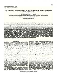
unsteady velocities and accelerations, and their estimates are very sensitive to the manner in which the data are smoothed. This study fitted cubic regressions to subsequent sections of the position data in order to smooth the estimates of position. This method is analogous to fitting a moving average (Webb, 1978; Frith and Blake, 1995; Harper and Blake, 1989, 1990; Domenici and Blake, 1991; Kasapi et al. 1992; Beddow et al. 1995; Franklin and Johnston, 1997) with the difference that we took a cubic fit where traditionally a linear fit has been used. The position data gave a series of N values where there were N frames in the sequence. For each frame j, a ‘smooth’ estimate of the position was given by the value h(j), where h(x) was the least-squares cubic regression for the x coordinates in frames j−n to j+n and the smooth width was 2n+1. The velocity and acceleration for each frame were given by the first and second differentials, respectively, of h(j) with respect to time. Smoothed results were not calculated for the first and last n frames in the sequence. The procedure was repeated for the data in the y direction. Where there was a maximum or minimum to the data, then the cubic fit would accurately match the peak values. The smooth width was still important; if it was too small, then peak values would contain digitizing uncertainty, and if it was too large then it would encompass several peaks and thus be unable to give a good fit to each one. The effect of the smooth width on the maximum velocity
300 Per cent of correct value
UK, in 1995; the Mediterranean scorpionfish Sc. notata and comber Se. cabrilla were caught and supplied by the Zoological Station, Naples, Italy, in 1997; the tropical blacksided hawkfish P. forsteri were imported from the Hawaiian Islands in 1996. In their natural habitats, these fish experience the following temperature ranges: Signy Island, Antarctica (60°43′S, 45°36′W), −2 to 1 °C; North Sea, 4–17 °C; Mediterranean Sea, 10–28 °C; Hawaiian Islands, 24–26 °C. Temperature-controlled aquaria in our laboratory maintained the fish at their respective median temperature, i.e. N. coriiceps and N. rossii at 0 °C, M. scorpius at 15 °C, Sc. notata and Se. cabrilla at 20 °C and P. forsteri at 25 °C. The numbers and sizes of the fish can be found in Table 1. Fish were held at these temperatures for at least 4 weeks prior to observations and were fed daily on krill, chopped squid or shrimp.
Amax
200 Vmax 95% limits
100
0 0
20
40 60 Smooth width
80
100
Fig. 1. Increasing the width of sequential portions of the cubic fit to the position data results in a decrease in the estimated maximum velocity Vmax and acceleration Amax. The smooth width of 43 for this sequence (vertical line) results in a fit where the digitizing errors have been smoothed, but the overall displacement data are preserved. The standard error of the smoothed positions from the raw data is 0.0015L (N=150), where L is total length for this smooth width. The standard error of the position of a reference point digitized from sequential frames is 0.00123L (N=80). The smooth width of 43 can thus be justified from the digitizing accuracy. The 95 % confidence limits of the velocity and acceleration data are shown by the shaded region.
1508 J. M. WAKELING AND I. A. JOHNSTON Vmax and acceleration Amax estimates can be seen in Fig. 1. As the smooth width increases, there is a sharp initial drop as the digitizing errors are smoothed. Next occurs a relatively level portion with the peaks and troughs being accurately fitted. Finally, the values of maximum velocity and acceleration decrease and the increasing smooth width causes oversmoothing. Values for the smooth width which gave accurate fitting of the maxima coincided with those that resulted in the standard error of the smoothed position data from the raw position data matching the standard error of repeatedly digitizing a point from the film (Fig. 1). Thus, we have confidence that the velocity and acceleration estimates were based on the correct degree of smoothing. The correct value for the smooth width depends on the digitizing accuracy. The correct smooth width also depends on the number of digitized frames per tailbeat or similar event which produces a fluctuation in acceleration. Smooth width was estimated independently for each species analysed here. Velocity and acceleration were determined for both the x and y directions, and the resultant was calculated as the total value. The acceleration estimate thus included the centripetal acceleration and did not necessarily take the same direction as the velocity. The tangential acceleration, which is the component of acceleration in the velocity direction, was also calculated. Rotational velocity and acceleration were estimated from the change in yaw angle in an analogous manner to the translational values, where yaw is the angle between the velocity vector and the spine at the position of the centre of mass ψ (see equation A33). Length-specific velocity Vˆ and acceleration Aˆ were calculated relative to the total body length L, where Vˆ=V/L and Aˆ=A/L, respectively. Power requirements during swimming Fast-starts are rapid acceleration events, and during the start the useful power Puse expended to move in a tangential direction can be approximated by the inertial power Piner, where: Puse ≈ Piner = (m + m a )VA
(1)
and m is the body mass, ma is the added mass of water that must be accelerated with the body, V is the velocity, and A is the acceleration. The added mass of water that moves with a fish during fast-starts has been estimated as ma=0.2m (Webb, 1982). The inertial power as described in equation 1 is that required for linear accelerations. The inertial power required for a rotational acceleration Piner,rot is given by a second relationship: Piner, rot = Iω a ,
(2)
where I is the moment of inertia of the fish [I=r2(m+ma)] about the centre of rotation, ω is the angular velocity, a is the angular acceleration, and r is the distance of the centre of mass of the fish from that centre of rotation. The tangential velocity V and
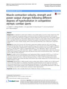
acceleration A are the following functions of the rotational values: ω=V/r and a=A/r, respectively. Substituting the values for I, ω and a into equation 2 reduces the expression for Piner,rot to the same as the translational inertial power Piner as given in equation 1. Inertial power was thus calculated from tangential velocity and acceleration regardless of whether the fish followed a linear or turning course. Translational inertial power estimates consider the acceleration of the centre of mass of the fish in the tangential direction. The centre of mass does not necessarily occur at a position along the spine; as a fish bends into a C-shape, the centre of mass moves away from the spine to lie within the space enclosed by the ‘C’. Weihs (1973) showed the fish centre of mass in its actual position, moving away from the spine during bending. Later studies, however, take it to occur at the same point along the spine as in a straight-stretched fish. The position vector q describing the true centre of mass is estimated by the mean position of 10 segments of the fish when each segment is given a weighting of its mass (volume): 10
q=
∑s(i )vi i =1
M
.
(3)
s(i) is the position vector for the centre of each segment (see equations A30–A32), vi is the volume for that segment as calculated for the straight fish (equation A9), and M is the total volume of the fish (equation A10). The effect of taking the actual centre of mass for the fish as opposed to that occurring along the spine can be seen in Fig. 2. Much of the initial movement of the spine occurs because the fish bends and does not represent a net displacement of the centre of mass. The course of the centre of mass is much straighter than that shown by the centre as positioned on the fish spine. Useful hydrodynamic power Puse (≈Piner) is expended to propel the fish in its direction of travel. However, as the body flexes, there is lateral motion; the total hydrodynamic power Pt is the total power expenditure during the movement both in the direction of travel and perpendicular to that direction. The hydrodynamic efficiency η is the ratio of the useful power to the total power: η=
Piner . Pt
(4)
Hydrodynamic efficiency has been estimated for a number of pike (Esox lucius) fast-starts by Frith and Blake (1995), who give values of η which relate Pt to useful hydrodynamic power and additionally give values of Piner calculated for the same sequence. The mean η for the pike fast-starts which related Piner to Pt is 0.31, and this value was used for the starts in the present study. Specific differences in kinematics may lead to specific differences in η; however, this will only be resolved when detailed hydrodynamic analyses of fast-starts are applied to a range of species. During swimming, the fish may rotate so that it does not face
Muscle power output and fast-start performance 1509 first complete muscle shortening cycle (as seen in the curvature plot, see Fig. 7). In almost all cases, the inertial power was positive. Negative inertial power did occasionally occur, corresponding to fish decelerations. However, assuming that such decelerations are passive during fast-starts, the mean power requirements were calculated solely from the positive contributions.
A B V (s −1)
4
0.240
2
0 150 0.192 A (s−2)
100
50 0.144 0 0.096
0.05
0.10
0.15 Time (s)
0.20
0.048 0
Fig. 2. (A) Spine positions for Myoxocephalus scorpius. Arrowheads indicate the snout, circles denote the position of the centre of mass as located on the spine, and numbers indicate the time (s) at which each image occurred. The solid blue line marks the displacement of the true centre of mass, the solid red line is the displacement of the centre of mass as located on the spine, and the dashed green line shows the displacement of the snout. (B) Non-dimensional velocity Vˆ and acceleration Aˆ estimates for the start shown in A. The blue lines are for the true centre of mass and the red lines for the centre as located on the spine. Solid lines are for tangential values, whereas the dashed line is the resultant of both tangential and centripetal acceleration.
its direction of travel. Yaw is taken as the angle between the velocity and the tangent to the spine at its centre of mass, lˆ1(m). Angular accelerations in yaw must be accompanied by turning torques, and the power for these can be calculated from equation 2, where I is the moment of inertia of the fish (equations A15–A17), and ω and a are the angular velocity and acceleration, respectively, of the yaw. The moment of inertia is taken from straight-stretched bodies and so will be an overestimate for that from C-shaped postures. Nonetheless, the mean power expended for the yaw in 10 fast-start sequences was a mere 0.001 % of the inertial power expended for those starts. The costs of yawing were thus ignored during this analysis. Mean inertial power was integrated for the duration of the
Muscle strain White muscle strain εw and activation was measured directly in N. rossii and P. forsteri during fast-starts using the sonomicrometry and electromyography (EMG) method described by Franklin and Johnston (1997). Pairs of sonomicrometry crystals implanted into the myotomal muscle measure the muscle length from the velocity of sound transmission between the crystals. Anaesthesia was initiated with a 1:5000 (m/v) solution of bicarbonate-buffered MS222 (ethyl m-aminobenzoate) and maintained by irrigation of the gills with a 1:3 dilution of this solution during surgery. Surgery was performed in a constant-temperature room set to the acclimation temperature of the respective species. Sonomicrometry and EMG measurements were taken from superficial rostral fibres at 0.35L, where L is the fish total length. For both species, previous dissections on dead specimens had confirmed that crystal positioning was in an alignment parallel to the surrounding fibres. Sonomicrometry data were also available for two other species recorded from our laboratory: N. coriiceps (Franklin and Johnston, 1997) and M. scorpius (G. Temple, unpublished data). Muscle strain was predicted additionally from the shape and curvature of the body. The strain at the edge of the planform fish silhouette corresponds to the strain at the lateral line of the fish. This is the region where the red, aerobic fibres occur. Where muscle fibres run parallel to the spine, then their strain ε can be calculated using trigonometry as: $$ , ε = bc
(5)
where bˆ (=b/L) is the length-specific distance from the spine to those fibres (half the width of the fish: see Appendix for methods of quantifying fish shape), and cˆ is the length-specific curvature of the spine at that location (equation A35). If the orientation of the red fibres is not parallel to the spine, then a correction should be made when calculating the strain (van Leeuwen et al. 1990) as oblique fibres undergo smaller strains than parallel fibres. The white fibres run in a helical arrangement deeper within the fish than do the red fibres (Alexander, 1969). This helical arrangement results in the strain being similar for white fibres at different depths; however, this strain may be less than that for the adjacent red fibres. The gearing ratio is the ratio of the red fibre strain to the white fibre strain for a given curvature of the body and was predicted to take a value of approximately 4 (Alexander, 1969). In the present study, the gearing ratio λ was estimated as the ratio of the mean white fibre strain ε¯w for a series of fast-starts (as measured using the sonomicrometry
1510 J. M. WAKELING AND I. A. JOHNSTON technique) to the corresponding mean red fibre strain ε¯red (as calculated by equation 5), where: λ=
εred εw
.
(6)
Deviations in red fibre orientation from parallel to the spine are ignored. This results in a slight overestimate in the gearing ratio. However, this error is not propagated into estimates for the white muscle strain. Validation of the techniques A set of six P. forsteri fast-starts was used to validate the quicker method of digitizing the spine position ‘by eye’ against the full method involving equations A18–A29 in the Appendix. If the calculated spine position is considered to be correct, then the position judged by eye resulted in mean errors of 1.8 % and 1.5 % increase in Vˆmax and lateral line strain, respectively, and – , respectively. The of 0.3 % and 1.1 % decrease in Aˆmax and P iner errors in velocity and acceleration, and therefore power, are smaller than those introduced by the smoothing technique (see Fig. 1), and so digitizing the spine by eye does not increase the uncertainty of the results. The errors for the strain estimates that are introduced by digitizing the spine by eye are similarly very small. If the mean white muscle strain ε¯w is set by a mean gearing ratio from equation 6, then there will be no difference between ε¯w for the two methods of estimating spine position. If the white muscle strain is set by an arbitrary gearing ratio, as has been the case for some other studies, then the difference between the two methods will be smaller than any error involved with the choice of gearing ratio. In vitro muscle mechanics Muscle contractile properties were determined for live fast fibre preparations from Sc. notata using the protocols described by Johnston et al. (1995), but with the following modifications. Preparations were isolated from the anterior abdominal muscles at a rostal position 0.35L along the fish. Fibres were dissected in a Ringer’s solution with the following composition (in mmol l−1): NaCl, 143; sodiun pyruvate, 10; KCl, 2.6; MgCl2, 1.0; NaHCO3, 6.18; NaH2PO4.2H2O. 3.2; Hepes sodium salt, 3.2; Hepes, 0.97; pH 7.3 at 20 °C. Both dissections and measurements were carried out at 20 °C. The length of the preparation was set to give maximal twitch. Preparations were frozen in isopentane cooled to −159 °C with liquid nitrogen. Frozen sections, 10 µm thick, were cut at several points along the preparation and stained for myosin ATPase activity (Johnston et al. 1974). Muscle mass was calculated from its volume (the product of length and cross-sectional area) assuming a density of 1060 kg m−3 (Mendez and Keys, 1960). Maximum contraction velocity V0 was determined using the slack test (Edman, 1979); fibres were given a step release during the plateau phase of an isometric tetanus sufficient to abolish force. V0 is the slope of the linear regression of step length against the time taken to redevelop force (6–8 step changes). Work-loop experiments were performed using single
sine waves. Cycle periods were tested in a range around 92 ms, the mean cycle period for the initial tailbeat as measured from ciné film. Fibre-length-specific peak-to-peak strain amplitude was set to 0.07, corresponding to that used by M. scorpius of similar size; the justification for this assumption is that the kinematics of these two species are similar (see Fig. 6). Two to three stimuli were given at a frequency of 260 Hz, which was shown to yield maximum tetanic force in preliminary experiments. Stimuli started just before peak length, with a duty cycle of 71.5–139.5 °. The passive work done by unstimulated fibres was always less than 4 % of the total work and was subtracted from the total work in each case. Statistics Least-squares linear regression was performed on sets of data to test the dependence of each parameter on the predictor variable. The kinematic parameters describing velocity, acceleration and power were all heteroscedastic and so were only tested after logarithmic transformation. Reduced major axis (Model II) regression was performed where the predictor was a random variable (Rayner, 1985), i.e. the nondimensional radius of the kth moment of volume lˆk(M) and Piner. A multivariate analysis of covariance tested the correlation between the kinematic parameters cˆ, εred, Uˆ and the fast-start performance parameters Vmax, Vˆmax, Amax, Aˆmax and Piner with the habitat temperature as a factor, where Uˆ is the lengthspecific velocity at which curvature travels along the body and Vˆmax and Aˆmax are the length-specific maximum velocity and acceleration of the fish, respectively. The fast-start performance parameters and Uˆ were all log-transformed owing to their heteroscedastic nature. Q10 values were calculated from the slopes of least-squares linear regressions on log-transformed data for kinematic parameters and temperature. Q10 values were calculated using the mean kinematic parameter for each and every species. All statistical tests were considered significant at a 95 % confidence level.
Results Body morphologies Length-specific fish chords are shown in Fig. 3. The various morphological parameters are given in Table 1 and shown in Figs 4 and 5 and provide a means to quantify differences between the shapes of the species. The non-dimensional radii of the moments of volume provide a good predictor of the nondimensional radii of the moments of mass (Fig. 4). The nondimensional radii of the moments of mass are predicted from the moments of volume by the following linear relationship: lˆk (m) = 1.065lˆk ( M ) − 0.033 ,
(7)
where k takes a value of 1 or 2 for the first and second moments, respectively. The predicted radii of the moments of mass deviate from the relationship in equation 7 with a
Muscle power output and fast-start performance 1511 0.2
Notothenia coriiceps
Notothenia rossii
Myoxocephalus scorpius
Scorpaena notata
Paracirrhites forsteri
Serranus cabrilla
0
b
0.2 0.2
0
0.2 0.2
0
0.2 0
0.2
0.4
0.6
0.8
l
1
0
0.2
0.4
0.6
0.8
1
l
Fig. 3. Length-specific body chord bˆ as a function of the non-dimensional length lˆ for the six species in this study.
standard error of 0.0025 and with an error never more than 0.0207. Some of this variation is interspecific, with different species having different density distributions throughout their 0.44 0.42 k=2
lk(m)
0.40 0.38 0.36 0.34 k=1 0.32 0.32 0.34 0.36 0.38 0.40
0.42 0.44
lk(M) Fig. 4. The non-dimensional radii of the first and second moments of mass lˆk(m) are predicted by the non-dimensional radii of the first and second moments of volume lˆk(M). Open circles, k=1; filled squares k=2. The line denotes the reduced major axis regression of lˆk(m) on lˆk(M) (see text for explanation), with r2=0.88, P=0.0003. The volume distribution of the fish body can thus be used as an estimate of the mass distribution.
body. Nonetheless, the centres of mass for straight-stretched fish can be estimated reliably from the centres of volume as measured using two orthogonal views of the fish alone. The relationships between the non-dimensional radii of the moments of area and volume are shown in Fig. 5. They are analogous to series given for the shapes of insect wings (Ellington, 1984). Relationships between the parameters have not been explained and have been termed ‘laws of shape: rules that are obeyed even if the reasons for doing so are unknown’ (Ellington, 1984). These relationships do, however, provide a good way to quantify body shape, and discrete clusters of points highlight specific morphologies (Fig. 5). The mean depth to slenderness of each species is given by the ratio Sˆl/Sˆp, where Sˆl and Sˆp are the non-dimensional longitudinal and planform areas, respectively (see equations A1–A4). In general, P. forsteri is a deep, slender fish, while M. scorpius is the opposite extreme, wide and shallow. The nondimensional radii of the moments of longitudinal area, lˆ1(Sl) and lˆ2(Sl), show distinct groups for each species. The two species , Sc. notata and M. scorpius, have the greatest proportion of longitudinal area in their head region, with M. scorpius having the relatively deepest head. The length-specific estimate for the centre of mass lˆ1(M) is similarly most anterior for these two species. N. rossii also has a low value for lˆ1(M) because it has a having a relatively broad head, as shown by its low nondimensional radii for the first and second moments of planform area lˆ1(Sp) and lˆ2(Sp).
1512 J. M. WAKELING AND I. A. JOHNSTON 0.62
0.52 0.50
0.58
0.46
l1(Sl)
l1(Sp)
0.48
0.44
0.54 0.50
0.42 0.46 0.40 0.38
0.42 0.34
0.32 0.34 0.36 0.38 0.40 0.42 0.44 0.46 l2(Sp)
0.38
0.42
0.46
0.50
0.54
l2(Sl)
0.55
0.48 0.46
0.53
l1(M)
l1(Swet)
0.44 0.51
0.42
0.49 0.40 0.47 0.45 0.38
0.38
0.40
0.42
0.44
0.46
0.48
l2(Swet)
0.36 0.31 0.33 0.35 0.37 0.39 0.41 0.43 l2(M)
Fig. 5. Distributions of the non-dimensional radii of the first and second moments of planform area lˆk(Sp), longitudinal area lˆk(Sl), wetted area lˆk(Swet) and volume lˆk(M). The reduced major axis coefficients of determination (r2) for these distributions are 0.93, >0.99, 0.99 and 0.97, respectively, with P