Music Structure Segmentation using the Azimugram ...

Dublin Institute of Technology

ARROW@DIT Conference papers

Audio Research Group

2007-10-01

Music Structure Segmentation using the Azimugram in conjunction with Principal Component Analysis Dan Barry Dublin Institute of Technology, [email protected]

Mikel Gainza Dublin Institute of Technology, [email protected]

Eugene Coyle Dublin Institute of Technology, [email protected]

Recommended Citation Barry, D., Gainza, M., Coyle, E.: Music Structure Segmentation using the Azimugram in conjunction with Principal Component Analysis. Audio Engineering Society, 123rd Convention, October 5–8 2007, New York, NY, USA.

This Conference Paper is brought to you for free and open access by the Audio Research Group at ARROW@DIT. It has been accepted for inclusion in Conference papers by an authorized administrator of ARROW@DIT. For more information, please contact [email protected], [email protected].

This work is licensed under a Creative Commons AttributionNoncommercial-Share Alike 3.0 License

Audio Engineering Society

Convention Paper Presented at the 123rd Convention 2007 October 5–8 New York, NY, USA The papers at this Convention have been selected on the basis of a submitted abstract and extended precis that have been peer reviewed by at least two qualified anonymous reviewers. This convention paper has been reproduced from the author's advance manuscript, without editing, corrections, or consideration by the Review Board. The AES takes no responsibility for the contents. Additional papers may be obtained by sending request and remittance to Audio Engineering Society, 60 East 42nd Street, New York, New York 10165-2520, USA; also see www.aes.org. All rights reserved. Reproduction of this paper, or any portion thereof, is not permitted without direct permission from the Journal of the Audio Engineering Society.

Music Structure Segmentation using the Azimugram in conjunction with Principal Component Analysis 1

2

3

Dan Barry , Mikel Gainza , and Eugene Coyle www.audioresearchgroup.com 1

Audio Research Group, Dublin Institute of Technology, Kevin St., Dublin 8, Ireland [email protected]

2

Audio Research Group, Dublin Institute of Technology, Kevin St., Dublin 8, Ireland [email protected]

3

Audio Research Group, Dublin Institute of Technology, Kevin St., Dublin 8, Ireland [email protected]

ABSTRACT A novel method to segment stereo music recordings into formal musical structures such as verses and choruses is presented. The method performs dimensional reduction on a time-azimuth representation of audio which results in a set of time activation sequences, each of which corresponds to a repeating structural segment. This is based on the assumption that each segment type such as verse or chorus has a unique energy distribution across the stereo field. It can be shown that these unique energy distributions along with their time activation sequences are the latent principal components of the time-azimuth representation. It can be shown that each time activation sequence represents a structural segment such as a verse or chorus.

1.

BACKGROUND

Music information retrieval is concerned with the automatic extraction of multi-level features from audio for the purposes of classification, comparison and segmentation. In particular, musical segmentation algorithms attempt to segment the audio timeline into perceptually salient events, such as the onset of a

particular instrument within the piece, or a key, rhythm or tempo change for example. In [1], Foote utilises an audio similarity matrix in order to find the boundaries between different consecutive self-similar segments. Other methods utilise Hidden Markov Models to segment the audio by clustering sequences of timbre states obtained from a dimensionally reduced constant Q representation of the audio [2]. Goto presents a method which detects the chorus of a song by using a

Barry et al.

Musical Structure Segmentation

chromagram representation [3]. The method aims to find the chroma vector which repeats most often in the song. In [4], the similar segments are detected by using MFCC features from overlapped audio frames. Perhaps one of the most useful forms of segmentation would allow the identification of the formal structural units of a musical piece, such as verses, choruses and bridges for example. Segmentation in this form would have applications in audio thumbnailing as well as fast audio browsing. Significantly fewer algorithms exist for this level of segmentation although [2][3] do approach this. 2.

METHOD

In this paper, a novel approach to structural segmentation is proposed, using the “azimugram” as the mid-level feature representation from which segmentation is derived. The azimugram is a timeazimuth representation of stereo audio which effectively shows the distribution of energy across the stereo field with respect to time. In this highly condensed domain, source location and intensity are clearly identifiable. Common music composition and production techniques often use additional or reduced instrumentation to herald a section transition in a song. This would suggest that source location and intensity will be highly correlated in similar sections within a given song. The distinct advantage of using the azimugram is the fact that it is invariant to both key changes and melodic variation within similar sections. Dimensional reduction in the form of PCA (principal component analysis) followed by ICA (independent component analysis) [5] is then applied to the azimugram. This combination of PCA followed by ICA is commonly referred to as ISA (independent subspace analysis). ISA has traditionally been used in source separation problems [6][7] but we show here that the technique has uses in segmentation also. Performing ISA on the azimugram results in a set of J independent basis function pairs where J is an estimation of the number of unique structural components present in the song, typically J < 5. Each of the J basis function pairs consists of one azimuth basis function and one time basis function of dimension r x 1 and t x 1 respectively, where r x t is the dimension of the azimugram. Taking the first pair as an example; the azimuth basis function corresponds to the most reoccurring energy distribution profile over time. The corresponding time basis function shows the activation sequence of this azimuth basis function. Each successive pair of basis functions will correspond to a unique energy distribution and time

activation sequence. This will be illustrated in section 2.2. Only the time basis functions are retained for further processing. Each time basis function is then smoothed using a low-pass filter. At this stage, each time basis function already exhibits a significant amount of structural information, whereby each one clearly represents a particular structural unit of the song such as a verse or a chorus. A final process is then applied whereby for any time instant, only the single largest value amongst all J time basis functions is assigned a value of one and all others a value of zero. This effectively enforces orthogonality between the functions which ensures that only one segment is active at any given point in time. Each of the J functions is now an independent binary sequence which represents the on/off sequence of a particular structural component of the song such as a verse, chorus, bridge or solo for example.

Figure 1: Block diagram of the music structure segmentation system. 2.1.

The Azimugram

Here, we coin the term “azimugram” to refer any time – azimuth representation of an audio signal. Such a representation shows the distribution of energy across the stereo field with respect to time. Azimugram representations can be created in various ways depending on the mixing model assumed. Much of the early work concerning azimuth calculation was based on models of binaural perception, whereby the azimugram is calculated by carrying out a cross correlation between the left and right inputs of the system on a multiband basis. The maximum outputs of the cross correlation functions correspond to the time lag of either the left or right input which can be resolved as an angle of incidence. An overview of binaural processors can be found in [8]. Later work in sound source separation [9][10][11], although not explicit, constructed azimugram variants from the short-time Fourier transform of stereo signals. Equations 1-3 below outline a basic technique to calculate an azimugram assuming an intensity stereo mixing model.

AES 123rd Convention, New York, NY, USA, 2007 October 5–8 Page 2 of 7

Barry et al.

Musical Structure Segmentation

Firstly, the log ratio of the left and right magnitude spectra is calculated resulting in a matrix of mixing coefficients A( n,t ) as in equation 1, where 1≤ n ≤ N , and N is the analysis frame size. These mixing coefficients are in dB format, whereby positive values refer to components which are dominant in the left channel and negative values refer to components which are dominant in the right channel.

X 1(n, t )

A(n, t ) = 20 Log 10

(1)

X 2 ( n, t )

where, X 1 ( n, t ) and X 2 ( n, t ) are the complex short time Fourier transforms of the left and right channels respectively. Theoretically, A( n,t ) will have values in the range of -96dB to +96dB for a 16bit recording. Following this, a weighted histogram of the mixing coefficients is created on a frame by frame basis. Firstly, the resolution, R, of the histogram is defined, where R specifies how many histogram bins are used to represent each half (left and right) of the histogram. For example, if R = 32, this will result in 2 x R discrete azimuth locations between far left and far right. Equation 2 below, converts the log spaced dB values into linear spaced discrete bin values which are used to populate the histogram created in equation 3.

  1  A(n, t ) = R ±  R −  A( n ,t ) / 6 × R   2  

(2)

where, 1≤ r ≤ 2 R , and where k represents the left or right channel indexed by 1 and 2, respectively. A more accurate way to calculate the azimugram can be found in [8]. This method uses phase information in addition to magnitudes resulting in slightly better localisation for concurrent sources overlapping in time and frequency. For segmentation purposes, the time resolution of the azimugram must be coarse enough to capture a representative energy distribution for a segment. Typically we use a frame size in excess of 3 seconds with a 50% overlap. Having a finer temporal resolution leads to details of instrument dynamics being exposed which can have adverse affects on the PCA stage used next. The assumption is that a similar stereo energy distribution can be observed over the course of a single segment, and that the same energy distribution should be apparent whenever that segment is active. In essence, verse 1 is assumed to have a similar stereo field energy distribution to verse 2 for example, and likewise with all other segments. As stated previously, the distinct advantage of using the azimugram representation is the fact that it is invariant to both key changes and melodic variation within similar sections. Typical values for R are in the region of 20 to 30 points, resulting in an azimuth resolution of 2 x R. With this time and azimuth resolution, the azimugram for a 4 minute song would be of dimension 40 x 160. Such a compact representation facilitates fast segmentation in the following stages.

where, 2R is the resultant histogram resolution and where,   denotes rounding up to the nearest integer. In equation 2 above, the term in brackets, preceded by ± , assumes the same sign as the current value of A( n , t ) . The matrix A( n,t ) now contains the mixing coefficients in a normalised integer format such that, 1≤ A( n, t ) ≤ 2 R . Using equation 3, each bin of the histogram, Az ( r ,t ) , is then populated by accumulating only the elements, n, of Xk ( n , t ) where A( n, t ) = r . 2

Az (r , t ) = ∑ k =1

I

∑ X (B , t) k

i =1

where B = n ∀ A( n, t ) = r

i

(3)

Figure 2: Azimugram of Romeo and Juliet – Dire Straits 2.2.

Independent Subspace Analysis

The next stage involves performing Independent Subspace Analysis on the azimugram. ISA is a technique used for dimensional reduction which involves performing PCA followed by ICA. The model assumes that the information contained within a data set, in this case the azimugram, can be represented by

AES 123rd Convention, New York, NY, USA, 2007 October 5–8 Page 3 of 7

Barry et al.

Musical Structure Segmentation

lower dimensional subspaces, the sum of which approximates the original data set. In the case of the azimugram, each subspace is the result of the product of two latent basis functions of dimension r x 1 and t x 1 respectively, where r x t is the dimension of the azimugram. Formally stated, it is assumed that the azimugram can be decomposed into a sum of outer products as in equation 4. J

J

j =1

j =1

Az = ∑ Az j = ∑ rj t Tj

overlap between the components. Logically, only one structural segment such as a verse or chorus should be active at once, and so theoretically, the basis functions should be mutually exclusive. In order to approach this, ICA is now performed on the time basis functions which results in a set of independent components as oppose to just decorrelated components. Figure 3 below shows the first 3 basis function pairs after PCA and ICA.

(4)

where T indicates the transpose of the matrix. In matrix notation, the azimugram Az, is represented as the sum of J independent azimugrams, each one corresponding to a particular structural segment of the song. The basis functions are obtained by carrying out singular value decomposition, commonly known as PCA, on the azimugram. This essentially transforms a high dimensional set of correlated variables into some number of lower dimensional sets of uncorrelated variables which are known as the principal components. The principal components are ranked in order of variance, so the first principal component contains the maximum amount of total variance present in the azimugram and each subsequent principal component represents the maximum remaining variance in the azimugram. Referring to equation 4, the principal components are represented by rj and t j . These basis function pairs represent the stereo field energy distributions and the time activations of each distribution respectively. One of the known issues with using PCA is that of choosing how many principal components to use to represent the data. In this application, the number of components, J , is set to be the expected number of reoccurring structures within the song. Typically, we use 3 principal components, expecting that there will be verses, choruses and other, where other will represent anything which is not a verse or chorus. Of course many other possibilities exist in musical composition, but 3 components should be sufficient to express the general structure of a typical song. In order to perform segmentation, only the time basis functions, t j , are retained. At this stage, the time basis functions are decorrelated but not independent. A limited amount of structure is already apparent within the time basis functions, but there is still activation

Figure 3: The decomposition of the azimugram in figure 2 into its first 3 independent subspaces. Here, r and t are the latent azimuth and time basis functions respectively. The independent subspaces are the result of the outer products of each basis function pair obtained using ISA. A known issue with the use of ICA is that the independent components returned can be arbitrarily scaled and/or sign inverted. For this reason, the independent components are normalised and positively oriented before proceeding to the next stage of processing. Following this, a lowpass filter is applied to each of the time basis functions in order to avoid the detection of short segments in the next processing stage. Another issue associated with the use of ICA is that the components could be returned in any order. For segmentation purposes, the components are ordered chronologically, i.e. in the order of time activation. We will refer to these normalised and lowpassed independent components as, t j ( t ) . 2.3.

Forcing Orthogonality

At this stage, some structure is apparent from the independent components whereby each component effectively represents the activation of a particular

AES 123rd Convention, New York, NY, USA, 2007 October 5–8 Page 4 of 7

Barry et al.

Musical Structure Segmentation

structure such as a verse or chorus but the boundaries between the segments are still unclear. In order to locate the segment boundaries more precisely, the independent components are converted into a set of binary functions by employing an ‘all or nothing’ scheme whereby for any time instant, the time basis function with the maximum energy is assigned a value of 1 and all others a value of 0 as in equation 5.

1 t j (t ) =  0

if t j (t ) > tm (t )   j≠m otherwise 

(5)

for 1 ≤ j ≤ J , where J is the number of basis functions. This effectively enforces mutual exclusivity. The binary time basis functions now represent the on/off sequence for each structure such as a verse or a chorus. Figure 3 below illustrates how each stage of processing leads to the resulting structural segmentation.

components. Performing ICA in the following stage clearly disambiguates this segment. For this example, the algorithm achieves a high degree of accuracy, correctly identifying the presence of all segmentation points with a maximum error of -6 seconds, corresponding to the early detection of the second chorus. This is attributed to the fact that the build up into the second chorus is quite prolonged. The instruments are layered more gradually prior to the actual onset of the second chorus. This is identifiable from the chorus plot in figure 4. Essentially the stereo field distribution at the end of verse 2 is more similar to the distributions observed in the choruses and so has been grouped as such during the PCA stage. The table below shows the automatically generated segment onset times along with the deviation from the manually annotated results.

T 1 2 3 2 3 2 3 1 2 3 1

Figure 4: First 3 time basis functions after PCA, ICA, lowpassing and binary selection. Note how the functions attain more structure after each stage of processing. Labeling was achieved manually. 3.

RESULTS

Referring to the example in figure 4 above, the frame size was set to approximately 6 seconds with an overlap of 50% resulting in a time resolution of 3 seconds. This essentially means that if a segmentation point is correctly detected within a frame, it will only be accurate to within 3 seconds of the actual segment onset. Analysing the above figure, it can be seen that using PCA alone leaves a significant amount of mutual information in the last 20 frames of the first 2 principal

Segmentation results for Romeo & Juliet Segment Actual* Algorithm* Deviation* Intro Verse 1 Chorus1 Verse 2 Chorus2 Verse 3 Chorus3 Inst. Verse 4 Error Outro

0:00 0:22 1:05 1:39 2:22 2:56 3:39 4:07 4:24 F.Det. 4:46

0:00 0:00 0:20 -0:02 1:02 -0:03 1:38 -0:01 2:16 -0:06 2:55 -0:01 3:36 -0:03 4:09 +0:02 4:24 0:00 4:42 N/A 4:45 -0:01 *time in minutes : seconds

Table 1: Comparison of manually annotated segment onset times (Actual) with automatically generated segment onset times (Algorithm). Also indicated is the manually annotated segment name. T indicates the basis function in which the segment was active. Given that the time resolution used in this example is 3 seconds per frame, the maximum error from the table above, -6 seconds, corresponds to only a single frame error. All other segmentation points have been identified within the correct frame with the exception of one false detection at 4:42 which does not correspond to any major structural change. This false detection can be explained by the momentary addition of an ornamental guitar line at that point in the song. The position of this guitar in the stereo field is such that the algorithm incorrectly attributes it to a chorus activation.

AES 123rd Convention, New York, NY, USA, 2007 October 5–8 Page 5 of 7

Barry et al.

Musical Structure Segmentation

The algorithm was also applied to a limited test corpus of popular recordings. The segment onset times for each recording were manually annotated. The automatic segmentation algorithm was then applied to each example and the results were compared. A correct detection was deemed to be within 6 seconds (2 analysis frames) of the manually annotated segment onset. A detection outside this range was considered as an incorrect detection. In this limited test case, the algorithm was able to achieve acceptable segmentation results 65% of the time. Table 2 summerises the results obtained.

4.

An algorithm capable of achieving automatic structural segmentation on stereo audio signals has been presented. The approach is shown to work well on intensity stereo recordings and to a lesser degree on convolutive recordings. The clear advantage of using the azimugram as the mid-level representation, is that it is invariant to key and melodic modulation which is common in music composition. Several problems still exist with the technique however. There is still a difficulty in knowing the exact number of principal components to use in the PCA stage. Added to this, the parameters of the lowpass operation after the ICA stage are still set manually. 4.1.

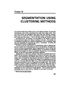
Table 2: Automatically generated segment onset times compared to manually annotated segment onsets. Although not the focus of this paper, some consideration should be given to the presentation of segmentation data to the user. The figure below shows the time alignment of the time domain waveform, the azimugram and a suggested visual representation of structural segmentation. Such a representation gives a user the ability to quickly navigate to important points within the musical piece.

CONCLUSIONS

Future Work

Other approaches for matrix decomposition such as locally linear embedding and non-negative matrix factorisation may be used instead of PCA. Although the current formulation is not applicable to mono recordings the same segmentation technique may also be applicable to other midlevel representations such as the chromagram for example. At present, the automatically generated segmentation points are near to the actual segment onsets but as yet are not perfectly aligned with lower level musical events such as bar lines or beats. This will be the topic of further work. 5.

ACKNOWLEDGEMENTS

This work is supported in part by the European Community under the Information Society Technologies (IST) programme of the 6th FP for RTD: The EASAIER project, contract IST- 033902. The work was also supported in part by Enterprise Ireland under the IMAAS project, reference CFTD/06/220. 6.

REFERENCES

[1] J. Foote, "Automatic audio segmentation using a measure of audio novelty," presented at Multimedia and Expo, 2000. ICME 2000. 2000 IEEE International Conference on, 2000.

Figure 5: Time domain, azimugram and automatic segmentation of Romeo and Juliet from Dire Straits.

[2] M. Levy and M. SANDLER, "New Methods in Structural Segmentation of Musical Audio " presented at Eusipco, 2006.

AES 123rd Convention, New York, NY, USA, 2007 October 5–8 Page 6 of 7

Barry et al.

Musical Structure Segmentation

[3] M. Goto, "A chorus-section detection method for musical audio signals," IEEE Workshop on Applications of Signal Processing to Audio and Acoustics 2003 [4] B. Logan and S. Chu, "Music summarization using key phrases," Acoustics, Speech, and Signal Processing, 2000. ICASSP'00. Proceedings. 2000 IEEE International Conference on, vol. 2, 2000. [5] A. Hyvarinen, J. Karhunen and E. Oja, "Independent Component Analysis", Wiley & Sons, 2001. [6] M.A. Casey, "Separation of Mixed Audio Sources by Independent Subspace Analysis," Proc. of the int. Computer Music Conference, Berlin, August 2000. [7] FitzGerald, D., Coyle E, Lawlor B., “Sub-band Independent Subspace Analysis for Drum Transcription”, Proceedings of the. Digital Audio Effects Conference (DAFX02), Hamburg, pp. 6569, 2002. [8] Stern, R.M., "An overview of models of binaural perception", 1988 National Research Council CHABA Symposium, Washington, D.C., USA, 1988. [9] Barry, D. and Lawlor, “Real-time Sound Source Separation using Azimuth Discrimination and Resynthesis”, Proc. 117th Audio Engineering Society Convention, October 28-31, San Francisco, CA, USA, 2004 [10] A. Jourjine, S. Rickard, O. Yilmaz, "Blind Separation of Disjoint Orthoganal Signals: Demixing N Sources from 2 Mixtures,” Proc. of IEEE Int. Conf. on Acoustics, Speech and Signal Processing, June2000 [11] C. Avendano, J.M. Jot, “Frequency-Domain Techniques for Stereo to Multichannel Upmix,” In Proc. AES 22nd International Conference on Virtual, Synthetic and Entertainment Audio, pp. 121-130, Espoo, Finland 2002.

AES 123rd Convention, New York, NY, USA, 2007 October 5–8 Page 7 of 7