JOURNAL OF ECONOMIC DEVELOPMENT Volume 27, Number 1, June 2002
Myopia, Liquidity Constraints, and Aggregate Consumption: The Case of Greece Konstantinos Drakos∗
In this paper we investigate the behaviour of aggregate consumption in Greece. In particular, we document the empirical failure of the Life-Cycle/Permanent Income Hypotheses. The empirical findings imply that this failure is due to the presence of Liquidity Constraints rather than Myopia.
I. Introduction Modelling consumption has attracted great interest, both on a theoretical as well as an empirical level. Traditionally, the benchmark theoretical framework for aggregate consumption has been given by the Life Cycle Hypothesis (LCH) developed by Modigliani and Ando (1963) and the Permanent Income Hypothesis (PIH) developed by Friedman (1957). A series of empirical papers has documented the basic theoretical framework’s inability to account for the observed consumption dynamics (Flavin (1981), Abel (1988), Campbell and Mankiw (1990), Bayoumi (1993), Shea (1995) to name just a few). Two explanations have been postulated for this failure. One explanation is that agents may be unable to borrow and lend freely; that is they may be liquidity-constrained (Zeldes (1989)). Another explanation is that agents are myopic and therefore fail to optimise in an intertemporal framework (Runkle (1991)). In the present paper we explore the dynamic behaviour of aggregate consumption in Greece. Recent studies on consumption in Greece have reported a failure of the LCH/PIH (Peleologos and Georgantelis (1992), Apergis et al. (2000)). In particular, Apergis et al. (2000) focus on the effects of deregulation in the Greek monetary sector on aggregate consumption. Using Granger causality tests they conclude that monetary decisions significantly affected consumption decisions only in the period following the deregulation. In particular, the report a significant increase both in the short and the long run sensitivity of consumption to money supply changes following the deregulation, while in contrast the corresponding sensitivities with respect to income changes have decreased. The present study is closer to the spirit of Peleologos and Georgantelis, (1992) who explore the validity of the LCH/PIH by testing whether consumption responds to anticipated changes in income, where anticipated income is proxied by an ARMA model. They employ aggregate data ∗ Department of Economics , Universit y of Essex, Wivenhoe Park, Colchester, CO 43 SQ, UK. Tel: 44-1206-872722, E-mail:
[email protected]. The author is grateful to an anonymous referee whose insightful comments have improved considerably the paper. Any remaining errors or ambiguities are the author’s responsibility.
97
JOURNAL OF ECONOMIC DEVELOPMENT
sampled annually for the period 1953-1988 and show that the LCH/PIH fails since (i) consumption does respond both to anticipated and unanticipated changes in income, and (ii) other macroeconomic variables such as inflation and its variability seem to affect consumption. The contribution of the present paper is twofold. First, given that no study has explored the sources of the LCH/PIH rejection we attempt to shed light on this issue by considering failures due to Myopia or Liquidity Constraints. Second, we extend the study of Peleologos and Georgantelis, (1992) by employing more recent data (including information from the 90s) and also by proxying anticipated changes in income by linearly projections on information available at the time of decision making (essentially using Instrumental Variables) instead of using an ad hoc ARMA model. The remainder of the paper is organised as follows. Section II reviews the theoretical background. Section III discusses the econometric methodology employed. Section IV presents the dataset employed. Section V discusses the estimation and the empirical results. Finally, Section VI concludes. II. LCH/PIH, Myopia and Liquidity Constraints: A Brief Review The LCH/PIH asserts that agents base their current consumption decisions on their expectations about their lifetime income, rather than their current income. This dissociation between current consumption and current income coupled with the Random Walk Hypothesis (Hall (1978)) implies that only ‘surprises’ in permanent income should affect current consumption, once lagged consumption is controlled for (Blinder and Deaton (1985)). More formally the benchmark model considers a representative agent who is assumed to maximise the expected value of a time-separable lifetime utility function. In each period t , the agent chooses consumption ( Ct ) and portfolio shares ( wj , t ) in order to: k
1 max Et ∑ U (Ct +k ) , k =0 1 + δ T −t
(1)
subject to:
(
M At +k = ( At+k −1 ) ∑ w j,t+k −1 1 + rj,t+k −1 j=1
) + Y
t+ k
− C t+ k ,
Ct+k ≥ 0 ,
(2)
AT ≥ 0
(3)
with k = 0,...,T − t , where U ( ⋅ ) is the one period utility function, Ct real consumption in period t , δ is the 98
DRAKOS: MYOPIA, LIQUIDITY CONSTRAINTS, AND AGGREGATE CONSUMPTION
rate of time preference. Et is the expectation operator conditional on information available at time t , T is the end of agent’s horizon, At
is the real end-of-period financial
(non-human) wealth of the agent in period t (after receiving income and consuming), r j,t is the ex post real after-tax return on the j th asset between periods t and t + 1 , wj ,t is
j , M is the number of available assets, and Yt is the real disposable labour income of the agent in period t . the share of end-of-period wealth held in the form of asset
As discussed in Zeldes (1989), analytic solutions to this problem when income is stochastic cannot in general be derived. Perturbation arguments can be used, however, to derive a set of first-order conditions (Euler equations) that are necessary for an optimum. In particular, these conditions should guarantee that an agent should be unable to increase expected utility by reshuffling consumption across periods. In algebraic form this condition results in:
(
)
U ′ (Ct+1 ) 1 + rj ,t U ′(Ct ) = Et , 1+δ (4) t = 1,..., T − 1, j = 1,..., M , where U ′ denotes the partial derivative of U with respect to C . If expectations are rational this leads to:
(
)
U ′(Ct +1 ) 1 + r j,t = 1 + e j ,t +1 , U ′(Ct )(1 + δ )
(5)
where e j ,t +1 is an expectational error orthogonal to elements belonging to the information set at time t . This Euler equation should hold with respect to any asset available including the riskless asset. Moving away from the benchmark now, under myopia, consumption should track current income. Therefore, any deviation from the LCH/PIH due to myopia should be symmetric. Consumption should exhibit equal sensitivity to predictable income increases and decreases (Shea (1995)). Altonji and Siow (1987) have shown that the presence of liquidity constraints implies an asymmetry in consumption behaviour. In particular, liquidity constraints imply that during periods of low income agents cannot sustain their optimal consumption plan by borrowing. Thus, since liquidity constraints impede borrowing but not saving, consumption should be more strongly correlated with predictable income increases than declines (Shea (1995)). III. Econometric Methodology Following Campbell and Mankiw (1990), and Shea (1995) one can test the LCH/PIH by running the following OLS regression (all variables are in natural logarithms): 99
JOURNAL OF ECONOMIC DEVELOPMENT
∆ ct = µ + λ∆yt + βrt + u t ,
(6)
where ∆ct is consumption growth, ∆yt is expected income growth, difference operator, rt
is the expected real interest rate and
ut
∆ stands for the is a well-behaved
disturbance term. Under the LCH/PIH, predictable income movements should not affect consumption, controlling for the return for saving. Thus, under the LCH/PIH, λ should equal zero provided ∆yt and rt are measured using information available at t − 1 . Under myopia, consumption should track income. In other words, consumption should respond symmetrically to predictable deviations of income from its mean. Under liquidity constraints, consumption should respond more strongly to predictable increases than decreases; liquidity constraints do not cause the Euler equation between adjacent periods to fail if optimal frictionless consumption growth exceeds expected income growth (Shea (1995)). Therefore, by slightly modifying model 6 one can test for the presence of liquidity constraints or myopia. In particular, this can be tested by running the following OLS regression: ∆ ct = µ + λ1 ( POS t )∆yt + λ2 (NEG t )∆yt + βrt + u t ,
(7)
where POS is a dummy variable for periods in which ∆ yt > 0 , and NEG is a dummy variable for periods in which ∆ yt < 0 . Under the LCH/PIH both λ1 and λ2 should equal zero. Under myopia the λ ’s should be positive, significant and equal. With liquidity constraints, λ1 should be significantly positive, and should be significantly greater than λ2 . Table A summarises the relevant testable hypotheses in terms of the parameters of Equation (7), derived under the validity of alternative models. Table A Model LCH/PIH Myopia
Testable Hypotheses λ1 = λ2 = 0 (i) λ1 = λ2, (ii) λ1 > 0, λ2 > 0 (i) λ1 > 0, (ii) λ1 > λ2
Liquidity Constraints
IV. Data The dataset consists of real disposable income (GDP less taxes) and real consumption at 1995 constant prices. The (ex post) real interest rate was constructed as the difference between the spot nominal interest rate for medium term deposits (3 to 12 months) and the change in the Consumer price Index (CPI). The data were sampled annually from 1960 to 1999 and were collected from the Ministry of National Economy of Greece and the IMF’s CD-ROM. The following figures depict the time series plots of real income and real consumption (left) and their first differences (right). 100
DRAKOS: MYOPIA, LIQUIDITY CONSTRAINTS, AND AGGREGATE CONSUMPTION
10.5
0.15
10.0
0.10
9.5
0.05
9.0
0.00
8.5
-0.05
8.0
-0.10 60
65
70
75 log(C)
80
85
90
95
60
log(Y)
65
70
75
80
First difference in log(C)
85
90
95
First difference in log(Y)
The time series plots of the level of series reflect their apparent non-stationarity and given their comovement one might strongly expect that they are linked by a long-run relationship (cointegrated). However, the present analysis is rather more interested with their short run behaviour as given by their first differences, which effectively also guarantee stationarity. The time series behaviour of changes in real consumption seems to track that of real income. The sample correlation between the two series is 0.76 (p-value 0.00). V. Estimation and Empirical Results 1. Estimation Methodology As it becomes apparent, the theory involves the predictable component of income growth and real interest rate, for which unfortunately, directly measured data is not available. Thus, one has to device a way of approximating the expected components of the variables. Following Cambell and Mankiw (1990) and Shea (1995) a way of circumventing this apparent difficulty is to estimate the parameters of Equations (6), and (7) by Instrumental Variables (IV). Following the literature, we use various information sets as instruments, such as lagged values of income growth, real interest rate, and consumption growth. Essentially, we project ex post changes on the information set available to consumers at the time of the decision making and hence extract the predictable component. 2. Empirical Results In order to test the validity of the LCH/PIH we first estimate model (6) where we restrict negative and positive income changes to exert a symmetric impact (if any) on consumption. We estimate the model1 described in Equation (6) by (i) OLS and (ii) IV obtaining:2
1. In all estimated models we account for the 1973 oil shock by the inclusion of an impulse dummy variable. 2. Unit Root tests are not reported for space conservation reasons. However, they are available upon request.
101
JOURNAL OF ECONOMIC DEVELOPMENT
Table 1 Estimation Results For: ∆ ct = µ + λ∆y t + β∆rt + δ(OIL ) + εt
µ λ
β R2 F-stat LM(1) ARCH(1) Sargan’s Instrument Validity Test
Model 1 (OLS) .0199 (4.92)*** 0.539 (8.38)*** 0.0014 (2.53)** 0.61 30.77*** 1.44 0.48 -
Model 2 (IV)
Model 3 (IV)
Model 4 (IV)
0.013 (1.83) 0.745 (4.09)*** 0.16E−3 (0.10) 0.57 24.62*** 0.30 0.42 0.001
0.017 (2.53)** 0.631 (4.56)*** −0.23E−3 (−0.15) 0.59 26.44*** 1.15 1.50 3.52
0.018 (2.72)** 0.623 (4.89)*** −0.30E−3 (−0.20) 0.58 26.10*** 1.03 1.56 6.98
Notes: (i) Model 1 is estimated by OLS, Models 2-4 Estimation Method Two -Stage Least Squares, (ii) Model 2 instrument list: three lags of income growth, Model 3 instrument list: three lags of income and interest rate changes, Model 4 instrument list: three lags of income, interest rate changes and consumption growth (iii) Sample: 1964 1999, (iv) White Heteroskedasticity -Consistent Standard Errors & Covariance, (v) OIL stands for an impulse dummy variable capturing the 1973 oil shock, (vi) Two (Three) asterisks denote significance at the 5% (1%) level.
The parameter of interest (λ ) when we employ standard OLS is significantly different from zero (t-stat 8.38) suggesting a value for the unconditional income elasticity of consumption d log(C ) ( εC,Y = ) of 0.53. This finding implies that movements in income affect d log(Y ) consumption growth. However, in order to test the implications of the LCH/PIH one needs to focus on predictable movements in income. We are enabled to do so by virtue of the models estimated by IV also reported in Table 1. The IV estimation results suggest that the elasticity is between 0.62 and 0.74 and is significant at all conventional levels. Thus, predictable movements in real income growth do exhibit significant explanatory power over consumption growth evidence which is against the validity of the LCH/PIH. In order to investigate the source of the LCH/PIH rejection, that is whether myopia or liquidity constraints are to blame, we use model (7) where we allow negative and positive changes in income growth to exert an asymmetric impact on consumption. However, before we report the estimation results one point is worth mentioning. As it becomes apparent from the time series plots of real consumption and real income the Greek economy has been on an expansionary trajectory over the past four decades. This creates an econometric problem since the actual number of negative changes in income is very small and might bias our econometric findings. In fact, real income has shrunk only in six occasions (out of 39 data
102
DRAKOS: MYOPIA, LIQUIDITY CONSTRAINTS, AND AGGREGATE CONSUMPTION
points, approximately 15% of the sample size). 3 So, bearing this in mind which might affect the statistical credibility of the analysis ,4 one has to be cautious in the interpretation of the empirical results. The estimation yields the following results presented in Table 2. Table 2 Estimation Results For: ∆ ct = µ + λ1 ( POS t )∆yt + λ2 (NEG t )∆yt + βrt + δ (OIL ) + εt
µ λ1 λ2
β R2 F-stat LM(1) ARCH(1) Sargan’s Instrument Validity Test F-stat H0: λ1 = λ2 = 0 H1: λ1 ≠ 0, λ2 ≠ 0
Model 1 (OLS) 0.016 (2.98)*** 0.589 (6.60)*** 0.283 (1.36) 0.001 (2.70)** 0.60 20.71*** 0.70 0.14 -
Model 2 (IV)
Model 3 (IV)
Model 4 (IV)
0.0134 (1.43) 0.740 (2.37)*** 0.658 (0.28) 0.11E−3 (0.04) 0.58 16.79*** 0.085 0.54 3.10
0.0135 (1.40) 0.696 (3.92)*** 0.240 (0.59) −0.176E−3 (−0.01) 0.60 18.70*** 0.84 0.65 2.99
0.011 (1.21) 0.733 (4.38)*** −0.003 (−0.07) 0.508E−4 (0.003) 0.59 17.94*** 0.52 0.53 4.74
95.93***
12.03***
21.57***
22.39***
Notes: (i) Model 1 is estimated by OLS, Models 2-4 Estimation Method Two -Stage Least Squares, (ii) Model 2 instrument list: three lags of incom e growth, Model 3 instrument list: three lags of income and interest rate changes, Model 4 instrument list: three lags of income, interest rate changes and consumption growth (iii) Sample: 1964 1999, (i v) White Heteroskedasticity -Consistent Standard Errors & Covariance, (v) OIL stands for an impulse dummy variable capturing the 1973 oil shock, (vi ) Two (Three) asterisks denote significance at the 5% (1%) level.
Moving to the hypotheses of interest, in all cases we are able to reject the joint hypothesis (LCH/PIH) that predictable negative and positive components of income growth do not affect consumption growth ( λ1 = λ2 = 0 ). However, it should be noted that individually it is only the coefficient of positive income growth that ‘drives’ the rejection. This highlights the problem caused by the relatively infrequent occurrence of negative income growth in the sample, as discussed above, which results to very high standard errors for the coefficient of
3. For compa rison purposes it is worth mentioning that Shea (1995) estimated a similar model using various samples of US consumption where the fraction of negative changes in consumption is between 1.6 percent and 14.7 percent. 4. The author is grateful to an anonymous referee for pointing this out.
103
JOURNAL OF ECONOMIC DEVELOPMENT
negative income growth. In terms of the absolute values of the estimated parameters consumption is more responsive to predictable positive changes in income, finding which is consistent with the case of liquidity constraints. Furthermore, the behaviour of consumption under the case of Myopia is not observed in the sample since the requirement that λ1 > 0 , λ2 > 0 is not satisfied given the statistical insignificance 5 of λ2 . In contrast, the data seem to be consistent with the predictions of the case of Liquidity Constraints. In particular, the robust finding of a significantly positive elasticity of consumption to positive predictable changes in income ( λ1 > 0 ) and the finding of an insignificant sensitivity to predictable negative changes in income ( λ2 = 0 ) provide evidence for the presence of Liquidity Constraints. All in all, the empirical findings point to a clear rejection of the LCH/PIH as far as the Greek case is concerned, a conclusion which is in accordance to the results reported in Paleologos and Georgantelis (1992) and Apergis et al. (2000). Moreover, we provide further evidence as to the possible reasons for the LCH/PIH’s empirical failure, which is due to Liquidity Constraints. Given the relatively underdeveloped financial market in Greece until the late 1980’s, with interest rates being heavily regulated by monetary authorities and also credit allocation decisions being heavily controlled, the case for Liquidity Constraints is even stronger. It was after the deregulatory actions adopted in 1988 which led to a liberalised financial sector. In fact, the present study can be viewed as complementary to Apergis et al. (2000) who explicitly studied the effects of deregulation on aggregate consumption and concluded that indeed there is a link between the two. VI. Conclusion Using aggregate data on consumption for Greece the paper investigated the reasons that underlie the rejection of the LCH/PIH. Allowing for potential asymmetries in consumption’s response to predictable income, the empirical findings suggest that the rejection of the LCH/PIH is driven by the presence of Liquidity Constraints. Future research would be more informative if micro data were employed in order to focus on the behaviour of households. However, for the moment, the unavailability of such dataset precludes such an econometric analysis.
References Abel, A. (1988), “Consumption and Investment,” NBER Working Paper No 2580. Altonji, J., and A. Siow (1987), “Testing the Response of Consumption to Income Changes with (noisy) Panel Data,” Quarterly Journal of Economics, 102, 293-328. Ando, A., and F. Modigliani (1963), “The Life-Cycle Hypothesis of Saving: Aggregate Implications and Tests,” American Economic Review, 53, 55-84. 5. Again recall that this coefficient is estimated very imprecisely (high standard errors).
104
DRAKOS: MYOPIA, LIQUIDITY CONSTRAINTS, AND AGGREGATE CONSUMPTION
Apergis, N., E. Varelas, and K. Velentzas (2000), “Money Supply, Consumption and Deregulation: The Case of Greece,” Applied Economics Letters, 7, 385-390. Bayoumi, T. (1993), “Financial Deregulation and Consumption in the United Kingdom,” Review of Economics and Statistics, 75, 536-539. Blinder, A., and A. Deaton (1985), “The Time Series Consumption Function Revisited,” Brookings Papers in Economic Activity, 2, 465-521. Campbell, J., and G. Mankiw (1990), “Permanent Income, Current Income, and Consumption,” Journal of Business Economics and Statistics, 8, 265-279. Deaton, A. (1991), “Saving and Liquidity Constraints,” Econometrica, 59(5), 1221-1248. Flavin, M. (1981), “The Adjustment of Consumption to Changing Expectations about Future Income,” Journal of Political Economy, 89, 974-1009. Friedman, M. (1957), A Theory of the Consumption Function, Princeton University Press, Princeton. Hall, R. (1978), “Stochastic Implications of the Life Cycle -Permanent Income Hypothesis: Theory and Evidence,” Journal of Political Economy, 86, 971-987. Paleologos, J., and S. Georgantelis (1992), “The Rational Expectations Approach to the Study of Consumption-Income Dynamics: The Case of Greece 1983-1988,” Rivista Internationale di Scienze Economiche e Commerciali, 39, 485-498. Runkle, D. (1991), “Liquidity Constraints and the Permanent Income Hypothesis,” Journal of Monetary Economics, 27, 73-98. Shea, J. (1995), “Myopia, Liquidity Constraints, and Aggregate Consumption: A Simple Test,” Journal of Money, Credit, and Banking, 27(3), 798-805. White, H. (1980), “A Heteroskedasticity-Consistent Covariance Matrix Estimator and a Direct Test for Heteroskedasticity,” Econometrica, 48(4), 817-838. Zellner, A. (1962), “An Efficient Method of Estimating Seemingly Unrelated Regressions and Test for Aggregation Bias,” Journal of the American Statistical Association, 57, 348-368. Zeldes, S. (1989), “Consumption and Liquidity Constraints: An Empirical Investigation,” Journal of Political Economy, 97(2), 305-346.
105