very-large-scale integrated circuit-manufacturing process. However, human judgment increases uncertainty in decision-making process. Tai et al. [5] assigned a ...
Proceedings of the World Congress on Engineering 2008 Vol I WCE 2008, July 2 - 4, 2008, London, U.K.
N-G Approach for Solving the Multiresponse Problem in Taguchi Method Abbas Al-Refaie, Ming-Hsien Li, and Chun-Wei Tsao
Abstract—The Taguchi method aims at reducing response variation from target so as to increase yields and product lifetime, reduce defects, and improve performance. However, the Taguchi method is only efficient for optimizing a single quality response. This research, therefore, proposes a neural network–grey relational analysis (hereafter abbreviated as N-G) approach for solving the multiresponse problem in the Taguchi method. The proposed approach includes two phases. The first phase utilizes neural networks to predict the normalized multiresponse values for all combinations of factor levels. Whereas, the second phase employs grey relational analysis to decide optimal combination of factor levels for multiresponse problem. A case study is provided for illustration. In conclusion, the N-G approach may provide a great assistance to practitioners for solving the multiresponse problem in real life applications on the Taguchi method. Index Terms—Neural Networks, Grey analysis, Taguchi method, multiresponse problem.
I. INTRODUCTION In practice, a great deal of engineering time is spent generating information bout how different design parameters affect performance under different usage conditions. The Taguchi [1] method is a widely accepted approach for robust design. The overall goal of robust design is to find settings of the controllable factors so that the response is least sensitive to variations in the noise variables, while still yielding an acceptable mean level of the response. Generally, a process’s or a product’s quality response can be divided into three main types: the smaller-the-better (STB); the nominal-the-best (NTB); and the larger-the-better (LTB) type responses. To optimize a quality response by the Taguchi method, an orthogonal array (OA) is utilized to reduce the number of experiments under permissive reliability. Then, signal-to-ratio (S/N) ratio is employed as a quality measure to decide the optimal combination of factor levels.
Manuscript received March 9, 2008. This work was supported by the Faculty of Engineering/ the Dept. of Industrial Engineering and Systems Management in Feng Chia University. A. Al-Refaie is currently pursuing the Ph.D. degree at the Dept. of Industrial Engineering and Systems Management in Fen Chia University, Taiwan. (Corresponding author e-mail: eng_jo_2000@ yahoo.com). M.H. Li is a professor in the Dept. of Industrial Engineering and Systems Management in Fen Chia University. C.W. Tsao is currently pursuing a M.Sc Degree at the Dept. of Industrial Engineering and Systems Management in Fen Chia University.
ISBN:978-988-98671-9-5
In today’s highly competitive markets, however, customers are concerned about more than one quality response. The Taguchi method has been extensively employed in manufacturing to robustly design a product or process with only one quality response [2-3]. Recently, the multiresponse problem in the Taguchi method has received an increasing research attention. For example, Phadke [4] employed pure engineering judgment for optimizing concurrently three quality responses in a very-large-scale integrated circuit-manufacturing process. However, human judgment increases uncertainty in decision-making process. Tai et al. [5] assigned a weight to the S/N ratio of each response then combined the multiresponses into a single performance index, which was then used to identify optimal combination of factor levels. In reality, it still remains difficult to determine and define a weight for each response. Pignatello [6] discussed a manufacturing process with five responses. They used data-driven transformations for each response variable in a multiple-univariate or one-at-a-time manner. Then, the regression technique based approaches were utilized to determine tentative optimal factor levels. Also, Reddy et al. [7] employed regression techniques based approaches during unifying goal programming to optimize simultaneously several responses. Regression approaches, however, increase the complexity of computational process. Thereafter, Antony [8] utilized principal component analysis (PCA) to transform the multiresponses in few uncorrelated ones, which were then employed for solving the multiresponse problem. However, PCA is based on some rigid assumptions, such as the error terms are multivariate normally distributed random variables, which may limit its use in practical applications. Jeyapaul et al. [9] utilized genetic algorithm for determining a weight for the S/N ratio of each response. Then, the weighted sum of S/N ratios was used to decide optimal factor levels. However, the genetic algorithm is a search heuristic that provides near optimal solutions for complex search spaces, such as scheduling and transportation problems. Artificial neural networks (NNs) and grey relational analysis have been broadly used for optimizing many a manufacturing process or a product. This research, therefore, provides a combined approach of artificial NNs and grey relational analysis for solving the multiresponse problem in the Taguchi method. Relevant background of NNs and grey relational analysis are introduced in Section II. The proposed approach is outlined in Section III. A case study is provided for illustration in Section IV. Finally, conclusions are made in Section V.
WCE 2008
Proceedings of the World Congress on Engineering 2008 Vol I WCE 2008, July 2 - 4, 2008, London, U.K. II. RELEVANT BACKGROUND A- Neural Networks The NNs mimic human brains to learn the relationships between certain inputs and outputs from experience. They are considered as information processing systems that have the abilities to learn, recall and generalize from training data. An NN is a parallel computing system consisting of many processing elements connected from layer to layer. An elementary neuron with R inputs is shown in Fig 1.
vectors is trained to adjust the weights in artificial NNs. For unsupervised learning NNs, a set of input vectors is proposed; however no target vectors are specified. For solving the multiresponse problem, therefore, the supervised learning NNs is appropriate for dealing with the multiresponse problem in the Taguchi method. The most extensively-used supervised learning network is the backpropagation (BP) model, which has been successfully applied to solve many problems [10-11]. Standard BP is a gradient descent algorithm in which the network weights are moved along the negative of the gradient of the performance function. Fig. 4 illustrates a basic BP neural network with three layers.
Fig. 1. Illustration of an elementary neuron. Each input is weighted with an appropriate w. The sum of the weighted inputs and the bias forms the input to the transfer function f. Neurons may use any differentiable transfer function f to generate their output. As shown in Fig .2, the transfer function can be logsin, tansig, or purelin.
Fig. 2. Types of transfer functions. In this research, a feedforward network will be used. A single-layer network of S logsig neurons having R inputs is shown in full detail on the left of Fig. 3 and with a layer diagram on the right.
Fig. 3. A single-layer network. Two types of learning NNs are respectively supervised and unsupervised. For supervised learning NNs, a set of training input vectors with a corresponding set of target
ISBN:978-988-98671-9-5
Fig. 4. A basic BP neural network. The BP neural network initially receives the input vector and directly passes it into the hidden layer. Each element of the hidden layer is used to compute an activation value by summing up the weighted input. The sum of the weighted inputs will be transformed into an activity level by applying a transfer function. Each element of the output layer is then used to calculate an activation value by summing up the weighted inputs attributed to the hidden layer. Next, a transfer function is used to estimate the network output. The actual network output is then compared with the target value. The BP algorithm refers to the propagation of errors of the nodes from the output to the nodes in the hidden layers. These errors are used to update the weights of the network. The most widely learning rule is the BP rule, in which the generalization property makes it possible to train a network on a representative set of input/target pairs and get good results without training the network on all possible input/output pairs. To test the network, a set of data are presented to the trained BP, and then the outputs are evaluated. Artificial NNs have been widely used for solving the multiresponse problem in many business applications. For example, Hou et al. [12] used neural networks and immune algorithms to find the optimal parameters for an IC wire bonding process. Huang and Tang [13] adopted NNs and genetic algorithms to optimize the multiresponse in As-Spun polypropylene yarn. Liao [14] proposed an approach based on NNs and data envelopment analysis (DEA) to solve the multiresponse problem in Taguchi method. B- Grey Relational Analysis Grey relational analysis, proposed by Deng [15], is a method of measuring degree of approximation among sequences according to the grey relational grade. Grey relational analysis is part of grey system theory, which is
WCE 2008
Proceedings of the World Congress on Engineering 2008 Vol I WCE 2008, July 2 - 4, 2008, London, U.K. suitable for solving the complicated interrelationships between multiple factors and variables. The major advantage of Grey theory is that it can handle both incomplete information and unclear problems very precisely. The grey relational analysis has been widely employed for solving the multiresponse problem in many manufacturing applications [16-18]. Based on the above introduction, this research proposes a combined approach using BP networks and grey relational analysis for solving the multiresponse problem in the Taguchi method. III. THE PROPOSED APPROACH The proposed N-G approach to solve for the multiresponse problem in Taguchi method is displayed in Fig. 5.
z ij
⎧ y ij ⎪⎪ = ⎨ T ⎪ − y ij + 2 ⎪⎩ T
y ij ≤ T
(3)
y ij > T
to be used for NTB response, where T is the desired target value. Step 2: Build a BP network to predict the zij values for all combinations of factor levels. Set the number of inputs equal to the number of controllable factors and set the input values as the values of factor levels. Set output values as the multiresponse values. Define the number of hidden layers, transfer functions, training parameters, and input data for prediction. Usually, the network parameter including the learning rate and momentum will be set to assist the trained network to attempt the convergence and stabilization in prediction behavior. An adaptive learning rate will attempt to keep the learning step size as large as possible while keeping learning stable. The learning rate is made responsive to the complexity of the local error surface. The stopping criterion is set to lower the root mean square error (RMSE) in training and testing process. Step 3: Let zoi denotes the reference sequence for response i; where the zoi value is equal to one in most applications, and zij be the specific comparison sequence. Let γ ( zoi , zij ) be the grey relational co-efficient for zij, which is calculated as Δ + ξ Δ max (4) γ ( z oi , z ij ) = m in Δ ij + ξ Δ max where ξ is the distinguishing coefficient of a value between zero and one, and commonly set value of 0.5. The Δ ij is the absolute deviation of the zij value from the reference zoi , or mathematically
Δij = z0i − zij Fig. 5. The steps of N-G approach. The main steps of the proposed approach are described as follows: Step 1: Normalize each quality response to avoid the effect of adopting different units and to reduce the variability. This is a necessary step before analyzing the data with the grey relational analysis. Let yij represents a response i (i=1,…, m) of experiment j (j=1,…, n). Let zij be the normalized value of yij, where zij lies between zero and one. Calculate zij using the appropriate formula from the Eqs. (1) to (3). yij − min ( yij , j = 1,..., n) (1) zij = max ( yij , j = 1,..., n) − min ( yij , j = 1,..., n)
max ( yij , j = 1,..., n) − yij max ( yij , j = 1,..., n) − min ( yij , j = 1,..., n)
to be used for STB response. Finally,
ISBN:978-988-98671-9-5
The Δ min and Δ max are the minimum and maximum values of Δ ij , respectively, from m responses for n experiments. That is, Δ min = m∀in min Δ ij i ∀j
(6)
and Δ max = max max Δ ij ∀i ∀j
(7)
Step 4: Let γ j be the grey relational grade for each experiment j. Calculate γ j using Eq. (8).
γj =
1 n ∑ γ ij n j =1
j = 1, … , n
(8)
Step 5: Let TGVl be the sum of the γ j values at factor level
to be used for LTB response. While, zij =
(5)
(2)
l. Calculate the TGVl for all factor levels. Typically, larger value of TGVl indicates better performance. Consequently, identify the factor level with the largest TGVl as the optimal level for that factor. A case study will be employed to illustrate the proposed approach in the following section.
WCE 2008
Proceedings of the World Congress on Engineering 2008 Vol I WCE 2008, July 2 - 4, 2008, London, U.K. IV. ILLUSTRATION
Step 3: The Δij values are calculated as 1 − z ji and also
This case study aimed at improving the performance of wire drawing process for SUS 304 using grey relational analysis based Taguchi method [19]. The main objective was to maximize concurrently the die life (hour abbreviated by hr) and wire tensile strength (kg/mm2). The orthogonal array L9 (34) was utilized to provide an experimental layout. In SUS 304 wire drawing process, three controllable process factors, including reduction ratio (A), lubricant temperature (B), and drawing speed (C), were investigated. The experimental data utilizing L9 (34) array are displayed in Table 1. The proposed approach was adopted to optimize the die life and wire tensile strength and described as follows:
listed in Table 2. From Table 2, the Δ m in and Δ m ax are equal to 0.997936 and 0.05768, respectively. The γ ( zoi , zij ) values are then calculated using Eq. (4). For
Step 1: Let z1j and z2j denote the normalized averages of die life ( y1 j ) and wire tensile strength ( y2j ), respectively, for each experiment j; j = 1, ..., 9. Since both quality responses are LTB type responses, the zij value is calculated using Eq. (1) and displayed in Table 1. For example, the z11 for die life in the first experiment is calculated as follows. The maximum values of y1 j and y2j are 75.37 hr and 250.3
example, γ ( zo1 , z11 ) for die life at the first experiment is calculated as 0.05768 + 0.5 * 0.997936 = 0.548277 γ ( z o1 , z11 ) = 0.5163 + 0.5 * 0.997936 The other γ ( zoi , zij ) values are obtained in a similar
manner. Step 4: The γ j values are calculated by Eq. (8) for all
experiments and listed in Table 2. For example, the γ 1 (= 0.461284) is the average of the γ ( z o 1 , z11 ) and
γ ( z o 2 , z 21 ) values; or (0.548277+0.37429)/2. other γ j values are obtained similarly.
The
Step 5: The TGVl values are obtained for all factor levels and depicted in Fig. 7.
kg/mm2, respectively. Whereas, the minimum values of 2 y1 j and y2j are 45.45 hr and 206.6 kg/mm , respectively. Then, the z11 is 65.58 − 45.45 = 0.673 z11 = 75.37 − 45.45 The other zij values are calculated similarly. Step 2: To investigate all the combinations of the threelevel factors, twenty-seven (= 33) experiments are needed as shown in Table 2. The BP network, shown in Fig. 6, is found the most efficient model to predict the zij values for all the 27 factor level combinations.
Fig. 7. The plot of TGVl value versus factor level.
Fig. 6. A BP network used for SUS case study. In Fig. 6, the BP network consists of three layers, including the input layer. The input layer contains the three process factors. Five neurons are assigned for the hidden layer. Finally, the output layer contains two outputs; the normalized averages of die life and wire tensile strength. Training is set for 10000 runs. The adaptive learning rate and momentum were initially set at 0.01 and 0.9, respectively. The mean square error (MSE) is used as stopping criteria. The network was then tested on actual inputs. The predicted zij values are also displayed in Table 2.
ISBN:978-988-98671-9-5
From Fig. 7, the combination of factor levels that optimizes the die life and wire tensile strength concurrently is identified as A3B1C3. In Table 1, the die life and wire tensile strength at A3B1C3 are 63.8 hr, which is above the overall average, and 250.3 (kg/mm2), which is the largest wire tensile strength obtained among all combinations of factor levels. This shows the efficiency of the proposed approach for solving the multireponse problem in SUS 304 wire drawing process. V. CONCLUSIONS An N-G approach is proposed and illustrated for solving the multiresponse problem in the Taguchi method. The main advantage of this approach is that it evaluates all of factor level combinations, and thus provides a global optimal combination is obtained with minimum resources.
WCE 2008
Proceedings of the World Congress on Engineering 2008 Vol I WCE 2008, July 2 - 4, 2008, London, U.K. Table 1. Experimental results of L9 (34) array for SUS 304 wire drawing process. Wire tensile strength (kg/mm2 )
Die life (hr)
Control factor Exp. j
A (%)
1
1
1
1
66.3
64.86 65.34 65.82
65.58
0.673
207.6
208.4
209.2
210.0
208.8
0.050
2
1
2
2
45.71 48.11 47.31 46.51
46.91
0.049
216.2
215.0
215.8
215.4
215.6
0.206
3
1
3
3
74.87 75.86 75.53 75.20
75.37
1.000
209.8
214.9
211.5
213.2
212.4
0.133
63.51
0.604
216.6
213.0
215.4
214.2
214.8
0.188
B C (°C) (m/min)
y1 j
Replicates (y1jk)
y2 j
Replicates (y2jk)
z1j
z2j
4
2
1
2
62.44 64.57 63.86 63.15
5
2
2
3
48.24 42.66 44.52 46.38
45.45
0.000
222.8
224.3
223.3
223.8
223.6
0.389
6
2
3
1
69.47 72.05 71.19 70.33
70.76
0.846
209.6
203.6
207.6
205.6
206.6
0.000
7
3
1
3
61.01 66.59 64.73 62.87
63.80
0.613
245.6
251.8
248.7
254.9
250.3
1.000
8
3
2
1
49.35 53.52 52.13 50.74
51.44
0.200
239.6
232.8
236.2
229.4
234.5
0.638
2
65.62 62.14
63.88
0.616
223.5
225.5
227.5
229.5
226.5
0.455
9
3 3 Overall average
63.3
64.46
60.74
221.5
Table 2. Grey analysis for predicted normalized responses. Control factor Exp. j
Phase I
Phase II
Normalized values
absolute deviation
Grey relational coefficient
Δ1 j
Δ2 j
γ ( zo1 , z1 j )
Grey grade
γ ( zo 2 , z2 j )
γj
0.548277
0.37429
0.461284
0.534993
0.378305
0.456649
0.936842
0.52244
0.387689
0.455064
0.41953
0.995063
0.606042
0.372581
0.489311
0.44435
0.988329
0.590096
0.374268
0.482182
0.46946
0.97266
0.574795
0.378253
0.476524
0.32858
0.997936
0.672647
0.371866
0.522257
0.0049
0.35128
0.995101
0.654689
0.372572
0.51363
0.62533
0.011584
0.37467
0.988416
0.637161
0.374246
0.505704
1
0.43174
0.15629
0.56826
0.84371
0.521583
0.41458
0.468082
2
0.4071
0.30599
0.5929
0.69401
0.509812
0.466604
0.488208
3
0.38292
0.51207
0.61708
0.48793
0.498767
0.564038
0.531403
A (%)
B (°C)
C (m/min)
1
1
1
2
1
1
3
1
4 5
z1j
z2j
1
0.4837
0.011759
0.5163
0.988241
2
0.45849
0.027543
0.54151
0.972457
1
3
0.43349
0.063158
0.56651
1
2
1
0.58047
0.004937
1
2
2
0.55565
0.011671
6
1
2
3
0.53054
0.02734
7
1
3
1
0.67142
0.002064
8
1
3
2
0.64872
9
1
3
3
10
2
1
11
2
1
12
2
1
13
2
2
1
0.52875
0.071694
0.47125
0.928306
0.573735
0.390008
0.481871
14
2
2
2
0.50349
0.15528
0.49651
0.84472
0.559177
0.414269
0.486723
15
2
2
3
0.4782
0.30438
0.5218
0.69562
0.545323
0.465975
0.505649
16
2
3
1
0.62365
0.031196
0.37635
0.968804
0.635938
0.379247
0.507592
17
2
3
2
0.59962
0.071189
0.40038
0.928811
0.618946
0.38987
0.504408
18
2
3
3
0.57509
0.15429
0.42491
0.84571
0.602512
0.413964
0.508238
19
3
1
1
0.38123
0.7425
0.61877
0.2575
0.498013
0.735851
0.616932
20
3
1
2
0.35766
0.87283
0.64234
0.12717
0.487728
0.889018
0.688373
21
3
1
3
0.33476
0.94232
0.66524
0.05768
0.478134
1
0.739067
22
3
2
1
0.47641
0.54592
0.52359
0.45408
0.544368
0.584071
0.56422
23
3
2
2
0.45125
0.74105
0.54875
0.25895
0.531296
0.734444
0.63287
24
3
2
3
0.42634
0.87198
0.57366
0.12802
0.518957
0.887813
0.703385
25
3
3
1
0.57334
0.3339
0.42666
0.6661
0.601373
0.477782
0.539577
26
3
3
2
0.54842
0.54403
0.45158
0.45597
0.585607
0.582915
0.584261
27
3
3
3
0.52326
0.73958
0.47674
0.26042
0.570507
0.733022
0.651764
ISBN:978-988-98671-9-5
WCE 2008
Proceedings of the World Congress on Engineering 2008 Vol I WCE 2008, July 2 - 4, 2008, London, U.K. REFERENCE [1]
G. Taguchi, Taguchi Methods Research and Development. Vol. 1. MI.: American Suppliers Institute Press, Dearborn, 1991. [2] C.C. Tsao and H. Hocheng, “ Comparison of the tool life of tungsten carbides coated by multi-layer TiCN and TiAlCN for end mills using the Taguchi method, “ Journal of Material Processing Technology, vol. 123, 2002, pp. 1–4. [3] M.H. Li, A. Al-Refaie, and C.Y. Yang, “DMIAC Approach to Improve the Capability of SMT Solder Printing Process,” IEEE Transactions on Electronics Packaging Manufacturing, to be published. [4] M.S. Phadke, Quality Engineering Using Robust Design. NJ, Englewood Cliffs: Prentice-Hall, 1989. [5] C.Y. Tai, T.S. Chen, and M.C. Wu, “An enhanced Taguchi method for optimizing SMT processes,” Journal of Electronics Manufacturing, vol. 2, 1992, pp. 91–100. [6] J.J. Pignatello, “Strategies for robust multiresponse quality engineering,” IIE Transactions, vol. 25, 1993, pp. 5–15. [7] P.B.S. Reddy, K. Nishina, and A. Subash Babu, “Unification of robust design and goal programming for multiresponse optimization- a case study,” Quality and Reliability Engineering International, vol. 13, 1997, pp. 371–383. [8] J. Antony, “Multi-response optimization in industrial experiments using Taguchi’s quality loss function and principal component analysis,” Quality and Reliability Engineering International, vol. 16, 2000, pp. 3–8 [9] R. Jeyapaul, P. Shahabudeen, and K. Krishnaiah, “Simultaneous optimization of multi-response problems in the Taguchi method using genetic algorithm,” International Journal of Advanced Manufacturing Technology, vol. 30, 2006, 870–878. [10] K. Lee, D. Booth, and P. Alam, “A comparison of supervised and unsupervised neural networks in predicting bankruptcy of Korean firms,” Expert Systems with Applications, vol. 29(1), 2005, pp. 1–16.
ISBN:978-988-98671-9-5
[11] Y. Liu, W. Liu, and Y. Zhang, “Inspection of defects in optical fibers based on back-propagation neural networks,” Optics Communications, vol. 198(4–6), 2001, pp. 369–378. [12] T.H. Hou, C.H. Su, and H. Z. Chang, “Using neural networks and immune algorithms to find the optimal parameters for an IC wire bonding process,” Expert Systems with Applications, 34, 2008, pp. 427–436. [13] C.C. Huang, and T.T. Tang, “Optimizing Multiple Qualities in As-Spun Polypropylene Yarn by Neural Networks and Genetic Algorithms,” Journal of Applied Polymer Science, Vol. 100, 2006, pp. 2532–2541. [14] H.C. Liao, “Using N-D method to solve multi-response problem in Taguchi,” Journal of Intelligent Manufacturing, vol. 16, 2005, pp. 331–347. [15] J.L. Deng, “Introduction to grey system,” Journal of Grey systems, vol. 1(1), 1989, pp.1–24. [16] C. L. Lin, J. L. Lin and T. C. Ko, “Optimisation of the EDM Process Based on the Orthogonal Array with Fuzzy Logic and Grey Relational Analysis Method,” International Journal of Advanced Manufacturing Technolology, vol. 19, 2002, pp. 271–277 [17] L.I. Tong and C.H. Wang, “Multi-response optimization using principal component analysis and grey relational analysis,” International Journal of Industrial Engineering-Theory Applications and Practice, Vol. 9(4), 2002, pp. 343–350. [18] C.-H. Wang1 and L.-I. Tong, “Quality Improvement for Dynamic Ordered Categorical Response Using Grey Relational Analysis,” International Journal of Advanced Manufacturing Technolology, vol. 21, 2003, pp.377–383 [19] A. Al-Refaie, M.H.C. Li, and K.C. Tai, “Optimizing SUS 304 wire drawing process by grey analysis utilizing Taguchi method,” Journal of University of Science and Technology Beijing, to be published.
WCE 2008