an expansion of the basic theory of cheirality [3], where in this case the ... picts the choice of 2 < k < n unique views from the set of n, there ... boundaries to form the view frustum. We will then .... formed by the planes passing through V0 and the joins of. V1 ΛV2 = L1 ... plane-at-infinity (for parallel planes) we will strip the last.
Polytopes, Feasible Regions and Occlusions in the �-view Reconstruction Problem David McKinnon½ , Barry Jones¾ and Brian C. Lovell½ ½ School of Information Techology and Electrical Engineering Intelligent Real-Time Imaging and Sensing (IRIS) Group University of Queensland ¾ Department of Mathematics University of Queensland
Abstract
-images has strong analogues with the set of the relevant subproblems of finding the intersection of 2 or more views �� � � � � � �� � ��½ � � � � � � �. Where �� � � � � � �� deunique views from the picts the choice of ¾� � � � set� of , there are � such choices. The notation for the �½ � is given as �½ � . Feasible re�� ������� � subsets of � gions and their � subregions have the inclusion relation �½ � � �½ � . �� ������� We can now answer our initial questions with the set notation. Firstly, which set of points in � ¿ can be reconstructed by the given camera orbit?
This paper asseses the question, given a arbitrary point in �¿ , can it be reconstructed by a given camera orbit? We show that a solution to this problem can be found by intersecting the view frustums of the cameras in the sequence creating a polyhedron that bounds the area in � ¿ observed by all cameras. For a projective set of cameras this can be considered as an expansion of the cheiral inequalities. We also show an exception to this basic principle is encountered when the point in � ¿ is occluded. Thus giving a weak condition for occlusion of an arbitrary point in � ¿ .
� � �
1 Introduction
� ����� ´��
�� µ ¾ �
�½ � �� �������
(1)
Secondly, which set of points in � ¿ can be reconstructed using all the given views from the camera orbit?
This work addresses the motivation to find the regions in
�¿ observed by two or more cameras in a given sequence.
� � �
We will refer to this common region as the feasible region for the given set of cameras, it represents the part of space where depth fusion may occur through triangulation. This is an expansion of the basic theory of cheirality [3], where in this case the inequalities are expanded to constrain a point to lie with the view frustum of each camera of interest. This work is also partly inspired be the treatment of polyhedral models in the computer graphics literature [5]. The following subsections introduce the basic concepts and notation maintained throughout the rest of the paper.
� ����� ´��
�� µ ¾ �
�½ � �� �������
(2)
Section 2 will explore the inequalities that bound these sets and section 3 will present a rudimentary algorithm to compute the bounds for an arbitrary camera orbit in projective space. Section 4 discusses some applications of the feasible regions.
1.2 Projective Geometry of Linear Features in � ¾ and �¿
1.1 Set Notation
This section will outline the notation and the basic building blocks for the representation of linear features in � ¾ and �¿. The development of the ideas in this section is heavily influenced by the notation and stucture of the linear features presented in [6], also drawing some similarities to the oriented matching constraints in [7].
The feasible region for views (� ½ � � � � � � ) will be denoted as the set �½ � of points (where �½ � � �¿ ) that project (un/occluded) into each of the -images. The problem of finding the feasible region for a sequence of 1
77
The first consideration when dealing with the multi-view geometry of linear features is their notation. Consistantly we will refer to features as any type of geometric object observed in a scene, be this points, lines or planes. Table 1 summarises the notation and degrees of freedom (DOF) for the group of linear features in the projective plane ( � �� � � � ). Hyperplane Points Lines
�
Ü Ü� ��
� �
�
�
Ü ¯ �� Ü Ü��� � Ü� �� ¯ �� Ü � Ü�
the image, when the feasible region suggests that the point should be observable within the view frustums.
2.1 Camera Model and View Frustum The pinhole camera model is the standard for modelling perspective distortion in image sequence. Perspective distortion is most prolific when a small focal length thus a greater Field of View (FOV), is employeed to model a scene that is both close to the camera and with a high depth variation. Firslty, we must consider the projection operator ( � ) or camera matrix that denotes the projection of linear features from the scene to the image plane ( � � �� � �� ). Table 3 summarises the range of projection operators for linear features.
DOF 2 1
Table 1. Linear features and there duals in � Similarly, Table 2 summarises the notation and the DOF for linear features in projective space ( �� �� �� �� � � ). Hyperplane Points Lines Planes
��
� ���� �����
�� �
� ��
Ü ¯���� Ü� Ü����� ���� Ü ¯���� Ü�� Ü���� ����� Ü ¯���� Ü��� Ü�
DOF 3 2 1
Hyperplane Point Line Plane
Table 2. Linear features and there duals in ��
��
Ü È� Ü� � � �� Ü È�� È��� � Ü���� -
� �� -
Ü��� � Ü
È���� È���� Ü���� È � Ü�
Table 3. Projection operators for linear features
These tables demonstrate the process of dualization for linear feature types via the antisymmetrization operator � � ��. The antisymmetrization operator should be considered as a determinantal method to generate the algebra for linear features, by performing an alternating tensor contraction over the space/s to which the operator is applied [?, ?]. The tensor notation will also convert directly into a computational scheme to evaluate the geometric entity in question. An important aspect of the tensor notation, is the ease at which linear features can be manipulated to form geometrically intuitive combinations of each other. The tables given above demonstrate this concept clearly, where lines are constructed from two points and planes (in � � ) are constructed from 3 points or a line and a point. This facet of the tensor notation (Grassmann-Cayley algebra) greatly increases it efficacy in solving for complex geometric configurations.
Generally it may be stated that � � � �� , where
is an arbitrary scale factor. The form of � for a regular point-to-point projection is,
� � �� � � �� �
(3)
�
� is rotation from the center of the world reference where � frame to the orientation of the camera and � is the location of the camera in the world reference frame. This depiction of the camera (3), is defined in a Euclidean metric and also assumes calibration of the internal parameters. The more general projective uncalibrated model differs according to � ) and projective collineation (� �� ) [1]. Thus, an affine (�� � � the calibrated model for point projection is,
2 Feasible Regions
�� � ���� ���� ����
(4)
� represents the internal parameters of the camera where �� � in an affine collineation,
In this section we will introduce the basic camera model (pinhole camera) and describe the process of projecting it’s boundaries to form the view frustum. We will then discuss the general intersection problem for 2 or more view frustum and give bounds for the number of differentally oriented solutions (cheirality), of which we will only be concerned with the positively oriented solutions. We will round-off this section by discussing the weak condition for occlusion of an arbitrary point in � � . We call this condition weak because it not geometrically based, rather it is based on a lack of the observation of the point in
����
�
�
� � � � �� ��� � � �
�
(5)
�
���� encorporate the focal length � into scale factors for conversion between metric distances (mm) and pixels, � is the skew of the CCD imaging array and � and �� are the coordinates of the cameras principal point [4].
2
78
where �� � ���« �¬ � � � ��« � �¬ � are the lines (edges) joining the vertices of the image plane. A further set of inequalities should also impose the image plane (although this is a largely redundant constraint) as another boundary and the cheiral inequalities (�’s). These boundary conditions are expressed as a set of algebraic inequalities for a given point �� ��, camera center � � and plane-at-infinity � ����� .
From this point, no assumptions will be placed upon whether the cameras are un/calibrated. Instead, we will implicitly assume that problems dealing with calibrated cameras will present image coordinates as they would be read �� ����� �� � �� ����) from the image plane ( and uncalibrated cameras present normalised image coordinates in a square centered fashion ( � � � �� � � � �) [2]. The ranges given for pixel coordinates typify the bounds for the camera. The projective (uncalibrated) assumption removes the ability to measure metric distances but can be made to preserve the orientation of an point-plane pair which we will see is the only requirement needed to build a proper view frustum. The view frustum for the camera is found by an inverse projection of the bounds of the camera into the scene. That is, a projection of the lines that bound the image plane, into their corresponding planes in the scene. Figure 1 demonstrates the labelling of the vertices and edges for the standard camera.
������ � � ��� � ������ � � ��� � ������ � � ��� � ������ � � ��� � � ��� � �� � �� ��� � � ����� ��� � ����� � � �
� � � �
� �
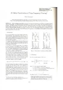
The scalars ( � ) ensure the cheirality (orientation) of each plane with respect to the view frustum. This is achieved by making sure each point in the view frustum has a positive projective distance from the camera (only the sign is important). The last two inequalities (�’s ) in (6) can be omitted from the boundary conditions if the scene points and cameras are know to be correctly oriented. Figure 2 shows some randomly generated positively oriented view frustums that have been clipped for display purposes. Note that not all of the cameras in this configuration are positioned to view the same part of space.
Figure 1. The labelling of the boundaries of projection for the standard view frustum.
Moving clockwise from the top left of the camera, the vertices � � �� � �� �� �� represent the corners of the image plane and � � is assigned to the cameras optical center (for finite cameras this is found as the nullvector of the camera matrix �� or � �� �� ��� ��� ����� ). The polyhedron formed by the planes passing through � � and the joins of
Figure 2. Four randomnly generated positively oriented view frustums for a square camera with a focal length of 1.
� � �� � � �� � �� �� � �� � �� �� �� � � ��, gives a set of boundary conditions for a point in � �, �
�
�
��
(6)
�
�
3
79
2.2 Feasible Regions and Cheiral Intersections
set of cameras. In summary we can consider the upper and lower bounds for the number of line-plane intersections for -views ( ) to be,
This section will move the discussion onto the case of multiple ( ) cameras. Running out of meaningful indices, our first step will be to rewrite (6) in a symoblic vector notation, feeling comfortable that we have an effective means to compute the various vectors in the inequalities.
�� � �� � �� �� � �� �� � �� �� � �� �� � � �� �� �
� � � � � � �
� ���
� �
� � � � � ��� �
(8)
the lower bound is the case of -views with the same internal camera parameters all lieing in the same position with the same orientation, this is clearly a critical configuration where no depth can be recovered. The upper bound is formed by the general case given by -views of a regular pinhole camera where the set of four lines from each camera must intersect each plane from each other camera. The intersection points will be positively and negatively oriented (ie. lie in front of the cameras and behind). Of the collection of intersection points formed in the planes, only a certain number will be valid (feasible) points. Valid points are those that conform to the inequalities given in (7). This is to say that we are only interested in positively oriented intersection points that lie on the boundary of the -view feasible region. An algorithm to find the intersection points that construct the bounding polyhedra will be considered in section 3.
(7)
The superscript on the vectors denotes the image number and the subscript reflects the labelling (Figure 1) of the planes (��� ), points (��� ) and plane-at-infinity (� ) where �� is the �� image plane. The inequalities given in (7) can now be considered to represent a valid set of points in the feasible region for the -view reconstruction problem (� � ) and the entire set of points that are�reconstructable (� � ) can be found as the union of the � subproblems (where � � � � n). This definition of the feasible regions for the -view reconstruction problem is tractable, however we are compelled to find a more definitive statement for the regions that captures their geometric structure more precisely allowing visualisation, volume calculations and a more compact representation. This is where we introduce the language of polytopes. Polytopes [8] allow us to represent the feasible regions as a convex hull of vertices (points), edges (lines) and facets (planes) in �� , thus providing a bounding polyhedra for the various linear programming problems implied by the application of the inequalities in (7). Since all planar intersections occur either before the plane-at-infinity or at the plane-at-infinity (for parallel planes) we will strip the last two inequalities ( ’s) along with the � �� (to cut down computation) from (7) leaving just the boundary conditions for the outer planes in the view frustums. The bounding polyhedra will be constructed from the intersection of pairs of the four remaining planes from� each camera (ie. lines �� � �� for camera there is �� such lines for each camera) with the set of four remaining planes in each other camera (� �� where �� ). In the general case there are two different ways that a line can intersect a plane. Firstly, if the points on the line and the plane are coplanar then their intersection will be the original line, or if the line and the plane are not coplanar then their intersection will result in a point. The points resulting from the line-plane intersections will form the vertices of the bounding convex hull representing the feasible region for a given
2.3 A Weak Condition for Occlusions The formulation for the feasible region given above will determine if a point lies within the intersection of the view frustums for the camera involved. However, this provides no indication as to whether the point of interest is occluded by some other object in the scene. This is brings us to consider a statement about whether a point that lies in a valid feasible region for a set of cameras is observable or not. Firstly, a strong statement of observability requires a precise model of the scene in question and typical ray casting process (analogous to a image-to-world graphics engine) can resolve geometrically whether there exists a clear line of site from the point in the scene to the image. Unfortunately, this strong statement of observability assumes that a complete 3D model has already been obtained. This is prohibitive for the purpose of building a 3D model from images, see we must seek another statement without this prerequisite. The weak statement of observability requires that the assumed texture surrounding the point in the scene is observable in the expected location in image. This statement is clearly less precise, but practically quite an acceptable means to determined whether a point has been occluded. With the discussion of the feasible regions above and this statement of observability a robust method to locate the images where a feature is present ensues. 4
80
3 An Algorithm to Compute the �-view Intersection Polytope
as sub/sequence closure. In this case a very valuable alignment of the same set of features can be achieved to correct any drift in the egomotion estimation up until that point. This philosophy has been used with great success in closed turntable sequences.
We present a rudimentary algorithm to find the bounding polytope containing the set of points Ë � for Ò-views. The algorithm is geometrically intuitive, but far from optimal for task. For an optimal approach refer to [?]. The algorithm will follow along the lines of the discussion given in the previous section for isolating the line-plane intersection points. Then, application of the first 4 inequalities in (7) will reveal the superfulous intersection points which are not feasible. Of the remaining points which will now lie on the convex hull of the feasible region’s polyhedra, edges must be selected to intersect points that lie only on a common plane of one of the view frustums. The proposed algorithm is given in Table (4).
1. 1.1 2. 3.
4.2 Path Planning Another perceived application of feasible regions is an autonomous robot fitted with either one or multiple cameras. If the robot is equipped with the mechanism to recognise certain objects in the scene (for our purpose we will imagine that these are polytope models), then the feasible region will allow the robots to plan a path around the object whereby the entire object of interest remains within the feasible regions of the camera at each time instant. Complex polyhedral objects can be represented as the convex hull of vertices encompasing the poylhedra, if each of the vertices is visible un/occluded in each view of the camera/s views then the robot has maintained a suitable perspective on the object. A robot fitted with cameras could then be instructed to model an entire area (at its own pace) making sure that it has gathered an adequate amount of information to fulfill the accuracy requirements of the mission.
Algorithm for the polyhedra bounding Find the � intersections, where � ������ Find the vertices � ����� �� � � �� �� �� � . Store the vertices that fulfill the first 4 inequalities (6). Find the edges from �� and the joins of �� in each plane.
�
Table 4. Proposed algorithm for calculating the bounding polyhedra for Ë �
4.3 Building Voxel Volumes The final application we have considered is building an arbitrary indexed voxel volume given a sequence of camera motions. Currently, the authors are yet see an application of voxel volume modelling where the voxel space has not been predesignated to house the object of interest. We feel that if the voxel volume 3D reconstruction technique is to reach its full practical value, the voxel spaces must be defined purely by the path of the camera, not placed at a point in space as a priori to reconstruction. Furhermore, information about the number of views that a feature is observable in and whether there are occlusions of the feature for a given path of the camera, is invaluable for the construction of the metric space and the subsequent optimisation problem for the building of the voxel volume.
4 Applications This section discusses some of the perceived applications of the concept of feasible regions in computer vision. It should be noted that this concept is very new and the authors are still considering the scope and application of the theory.
4.1 Object Querying The motivation here is to be able to query a sequence of images of a static scene (and the corresponding 3D reconstruction of the scene) to see if a feature lies within the view frustum of a given camera or a given set of cameras. Principally, we feel that this process may enhance the regular Structure From Motion (SFM) pipeline [?] with the ability to relocate lost or occluded tracks based on an expectancy for when they will return into the camera’s field of view. Another related application would be to retrospectively update the tracking profile of a feature found in image « to all the previous images where the feature was observable. This process could be used to great effect in the SFM pipeline for long sequences, where the camera completes a loop (ie. viewing the same area of the scene multiple times with some seperation in the exposure) which we will refer to
5 Conclusions and Future Work We have presented a novel idea that sets the boundary for points in space that are reconstructable by an arbitrary camera path. We have considered which points are reconstructable in the general case and which points are observable in every image. We have also shown that this formulation leads to a weak condition for occlusions. As a matter of future work the authors would like to consider the quality of observation for a point and the subse5
81
[8] G. M. Ziegler. Lectures on Polytopes. Graduate Texts in Mathematics, Springer-Verlag, 1994.
quent quality of reconstruction for a point given multiple observations. The envisaged formulation is to consider the expected error in the observation of a feature in the image and the projection of this error into space forming a cone. The intersection of multiple error cones gives something akin to a set of geodesic probability surfaces, representing the likelihood of the corresponding 3D feature lieing in this part of space. The introduction of such a concept would lead to a sophisticated method to determine the overall quality of reconstruction for the scene given a specific camera orbit. Then, points that are positioned poorly in the scene for reconstruction purposes can treated with a greater caution. In this manor the quality of reconstruction can be set as an input parameter to the SFM pipeline and made to replicate the average depth fusion for human vision. This can be considered as the ideal quality of reconstruction for visualisation with VR glasses. The authors are also looking into optimal algorithms to intersect the view frustums and create the resulting polyhedron.
6 Acknowledgements The authors would like to thank Carlos Leung and Ben Appleton for many interesting discussions on the development of the ideas presented in this paper. Also we would like to thank Bob Andrews for his assistance in editing this paper.
References [1] R. I. Hartley. Euclidean reconstruction from uncalibrated views. Applications of Invariance in Computer Vision - LNCS, 825:237–256, 1994. [2] R. I. Hartley. In defense of the eight-point algorithm. IEEE Transactions on Pattern Analysis and Machine Intelligence, 19(6):580–593, 1997. [3] R. I. Hartley. Chirality. Int. Journal of Computer Vision, 26(1):41–61, 1998. [4] R. I. Hartley and A. Zisserman. Multiple view geometry in computer vision. Cambridge University Press, 2000. [5] S. Savchenko. 3D Graphics Programming : Games and Beyond. SAMS Publishing, 2000. [6] W. Triggs. The geometry of projective reconstruction i: Matching constraints and the joint image. Int. Conf. on Computer Vision, pages 338–343, 1995. [7] T. Werner and T. Pajdla. Oriented matching constraints. 6
82