evidence shows that the debt crisis of the early 1980s and the Tequila crisis of. 1995 stalled a process ..... Yet the experience of Puerto Rico is also interesting, given that it is an economy that started with a similar ..... Government. Effectiveness.
Chapter 1
NAFTA and Convergence in North America: High Expectations, Big Events, Little Time William Easterly♣, Norbert Fiess ♦, and Daniel Lederman ♦ First Draft: October 2, 2002 This version: March 27, 2003
Abstract The negotiations of NAFTA in the early 1990s immediately raised high expectations for economic convergence in North America. These hopes were grounded in neoclassical economics. This paper examines the evidence concerning the impact of NAFTA on economic convergence in North America. Any such analysis is hampered by the big-events-little-time problem, which makes the identification of the NAFTA effect difficult due to contemporaneous big shocks and the relatively little time that has transpired since 1994. Time series evidence shows that the debt crisis of the early 1980s and the Tequila crisis of 1995 stalled a process of convergence that might have accelerated after trade liberalization in Mexico and NAFTA. Cross-country evidence indicates that a substantial share of the current income gap between the U.S. and Mexico can be explained by an institutional gap. Panel data evidence indicates, nevertheless, that NAFTA might have had a substantial effect on manufacturing TFP convergence. But initial conditions determined which regions within Mexico benefited the most, and thus the post-NAFTA period has been characterized by economic divergence within Mexico. We conclude that NAFTA has been helpful but free trade alone will not necessarily lead to economic convergence in North America.
♣
Department of Economics, New York University The World Bank, Office of the Chief Economist for Latin America ♦ We are grateful to Craig Burnside, Gerardo Esquivel, Andrew Harvey, Ernesto López-Córdova, William Maloney, Miguel Messmacher, Guillermo Perry, Maurice Schiff, and Luis Servén for helpful discussions and comments on earlier versions. We also benefited from the criticisms provided by two anonymous referees. The opinions expressed in this paper belong to the authors and they do not represent the views of the World Bank. ♦
Contents 1.
Introduction and Related Literature .................................................................................... 4 1.1 High Expectations ................................................................................................................. 5 1.2 Technology and Divergence: The “Big” Story ..................................................................... 5 1.3 Geography and Divergence: The “Big” Story....................................................................... 6 1.4 Life after NAFTA: Big Events, Little Time.......................................................................... 6 2. Time Series Evidence.............................................................................................................. 7 1.2.1 Structural time series modeling.......................................................................................... 7 1.2.2 Cointegration analysis ........................................................................................................ 9 3. Income Gaps and Institutional Gaps ................................................................................. 13 1.3.1 Data and Methodology ..................................................................................................... 14 4. Productivity Gaps within Industries, across the U.S. and Mexico........................................ 19 1.4.1 Data and TFP Estimates ................................................................................................... 20 1.4.2 Estimation Strategy .......................................................................................................... 21 1.4.3 Results .............................................................................................................................. 22 5. Initial Conditions and Divergence within Mexico ............................................................ 23 1.5.1 Data and Methodologies................................................................................................... 23 1.5.2 Results .............................................................................................................................. 25 6. Conclusions and Final Remarks........................................................................................ 28 References ..................................................................................................................................... 31 Appendix ....................................................................................................................................... 35
Figures and Tables Figure 1. GDP per Capita Relative to the U.S., Selected Economies, 1960-2001.......................... 4 Figure 2. The U.S.-Mexico GDP per Capita Gap: Similar-Cycle Model with Quarterly PPP Adjusted Data, 1960-2000............................................................................................................... 9 Table 1: Cointegration Analysis for US-Mexico, 1960 Q4 - 2000 Q4 ..................................... 10 Figure 3. Trace Tests for Cointegration between U.S. and Mexico (Log) Quarterly GDP, 1960Q4-2000Q4 (recursive estimates).......................................................................................... 11 Figure 4. Mexico Year Effect Minus LAC Year Effect, Log (GDP pc/US GDP pc)(PPP).......... 12 Figure 5. Institutional Gaps in North America, 2000/01............................................................... 13 Table 2. Regressions of Log GDP per Capita 2000 (robust standard errors in parentheses).... 15 Figure 6. The Contribution of Institutional Gaps to the U.S.-Mexico Income Gap...................... 17 Figure 7. Mexico Year Effects relative to LAC Year Effects, Institutional Index (ICRG) .......... 18 Table 3. Institutional Changes in Latin America ...................................................................... 19 Figure 8. Evolution of U.S.-Mexico Productivity Differentials by Industry, 1976-2000 ............. 21 Table 4. Did NAFTA Accelerate Manufacturing TFP Convergence? Arellano-Bond GMM Differences Regression Results for data from 1980-2000 ........................................................ 22 Figure 9. Ratio of State GDP per Capita Relative to the Distrito Federal, 1940-2000 ................. 24 Table 5. Potential Determinants of Growth of GSP per Capita, 1990-2000............................. 25 Figure 10. Relationship between Growth (1990s) and Public Employment in Mexican States: More is not necessarily better........................................................................................................ 27 Figure 11. Patents Granted to Mexican Residents by the U.S. PTO, 1980-2000 ......................... 29 Figure 1A: Quarterly Data Used for Time Series Analyses.................................................................. 35 Table 1A. List of Codes and Industries Used in TFP Convergence Analysis .................................... 36 2
Table 2A. Summary Statistics of Variables and Data Used for TFP Convergence Analysis, by Country and Industry (standard deviations in parentheses) ........................................................................... 37 Table 3A. Summary Statistics for Data Used for Analysis of Institutional Gaps and Income Gaps ..... 37 Table 3A. Summary Statistics for Data Used for Analysis of Institutional Gaps and Income Gaps ..... 38 Table 4A. Summary Statistics for Data Used for Econometric Results Presented in Figures 4 and 7 on Institutional Gaps and Income Gaps .............................................................................................. 38 Table 5A. Groups of countries used to calculate GDP and institutional gaps in Figures 4 and 7 ......... 38 Table 6A. Data Used for Analysis of Convergence Across Mexican States during 1990-2000 ........... 39 (all variables are in logs, except the poor states dummy) ................................................................. 39
3
1.
Introduction and Related Literature
The North American Free Trade Agreement (NAFTA) was formally implemented on January 1, 1994 by the United States, Canada, and Mexico. This treaty instantly gained global notoriety since the formal negotiations started in 1991 mainly because the initiative would become not only one of the most comprehensive trade agreements in history, but also because it seemed to be a breakthrough by leading to free trade in goods and services among developed countries and a developing country. The high expectations were that trade liberalization would help Mexico catch-up with its Northern neighbors. As shown in Figure 1, the ratio of Mexican GDP per capita to the U.S. did increase after unilateral trade reforms were implemented in 1986 and also after the implementation of NAFTA in the aftermath of the so-called Tequila crisis. However, it is noteworthy that other Latin American economies also grew faster than the U.S. economy since the mid-1980s, especially Chile and to a lesser extent Costa Rica. Thus it is not obvious that NAFTA was particularly important in helping Mexico catch-up with the United States. Yet the experience of Puerto Rico is also interesting, given that it is an economy that started with a similar level of development as Mexico in the late 1950s, but achieved an unprecedented level of economic and institutional integration with the U.S. in 1952, and subsequently experienced the fastest rates of economic growth in the developing Latin American economies. This paper attempts to assess the extent to which these high expectations seem to be materializing. It examines trends and determinants of income and productivity gaps observed in North America, both across countries as well as within Mexico. Figure 1. GDP per Capita Relative to the U.S., Selected Economies, 1960-2001 0.60
0.40 Mexico Brazil Puerto Rico Costa Rica Chile Argentina Colombia
0.30
0.20
0.10
20 00
19 98
19 96
19 94
19 92
19 90
19 88
19 86
19 84
19 82
19 80
19 78
19 76
19 74
19 72
19 70
19 68
19 66
19 64
19 62
0.00 19 60
GDP per Capita (ppp) over US GDP per Captia
0.50
Source: Loayza et al. (2002), World Penn Tables 5.0, and World Development Indicators.
4
1.1 High Expectations The high expectations for NAFTA were supported by neoclassical growth and trade theories. The seminal work of Solow (1956) states that capital-poor countries grow faster than rich countries due to the law of diminishing returns, as long as production technologies, population growth, and preferences are the same across countries. Likewise, the neoclassical Hecksher-Ohlin trade models predict that as the prices of goods and services converge, so will factor prices, including real wages. Hence income levels across borders will also tend to converge as prices converge. A key simplifying assumption of neoclassical economics is that all countries use the same production technologies exhibiting either constant or diminishing returns to scale. There is a lively debate about the evidence concerning the impact of trade liberalization on income convergence across countries (Slaughter 2001; Ben-David 2001, 1996). There is also an extensive literature about economic convergence within countries including Barro and Xala-IMartin (1995) and Xala-I-Martin (1996). At least since the publication of Barro (1991), the economics profession has been aware that convergence might be conditioned by convergence in certain fundamentals that are believed to cause economic growth. While there is admittedly much uncertainty about what these fundamentals are (Doppelhofer et al. 2000), the evidence of conditional convergence can be interpreted as evidence in favor of the neoclassical growth model or as evidence that there are fundamental differences that prevent income convergence. 1.2 Technology and Divergence: The “Big” Story For Easterly and Levine (2001) and Pritchett (2000), the “big story” in international income comparisons is that the rich have gotten richer while the poor got poorer. Some studies focusing on cross-country differences in the levels of income per capita (or GDP per worker) argue that these differences are largely explained by institutional factors (Hall and Jones 1999; Acemoglu, Johnson, and Robinson 2001). However, there are other factors, besides different fundamentals that might impede economic convergence among geographic areas even if there is free trade. More recent theories of growth with increasing returns and/or technological differences across regions, such as the pioneering work of Romer (1986, 1990), Lucas (1988), and Grossman and Helpman (1991), predict divergence in income levels and growth rates across regions. Trade flows might help international technology diffusion when technical knowledge is embodied in goods and services, and theories of technology diffusion via trade have been the subject of a fastgrowing literature (Eaton and Kortum 1999, Keller 2001). A related literature focuses on the barriers that impede technological adoption, which explain differences in the levels of income per capita (Parente and Prescott 1996). Thus, even when production technologies are different across countries, convergence can be aided through the liberalization of trade. But this would tend to be detected in convergence (divergence) of TFP levels within industries across countries (Bernard and Jones 1996). But even if trade liberalization allows poor countries to import production technologies from advanced countries, if the factor endowments are different, productivity levels might not converge due to the mismatch between labor skills available in poor countries and the sophisticated technologies imported from the rich countries. Hence productivity gaps within industries across countries might persist even if trade facilitates technological convergence (Acemoglu and Zillibotti 2001). 5
1.3 Geography and Divergence: The “Big” Story The recently resurgent literature on economic geography, transport costs, economies of scale, and knowledge spillovers is less optimistic about the impact of trade liberalization on economic convergence (Krugman 1991; Fujita, Krugman and Venables 1999). For example, transport costs will remain as barriers to trade and economic integration even if all policy distortions are removed (Eaton and Kortum 2002). In addition, if learning and innovation depend on trade, then geography will also be an impediment to convergence via technological diffusion (Keller 2002; Eaton and Kortum 2002). These factors might hamper income convergence across countries (Redding and Venables 2001). Moreover, economies of scale and knowledge spillovers might make some geographic regions more prosperous than others simply because of the cumulative effects of initial conditions such as the density of economic activity (Ciccone and Hall 1996). 1.4 Life after NAFTA: Big Events, Little Time On the day of NAFTA’s implementation, the Zapatista rebels took up arms in Mexico’s southern state of Chiapas. Later that year, in December 1994, Mexico was forced to float the Peso, which was followed by a deep banking crisis and severe recession. Beginning in late 1995, after a sharp deterioration and subsequent recovery of domestic investment, the Mexican economy was recovering by 1996 (Lederman et al. 2003). These were big events that coincided with the implementation of NAFTA. Moreover, from a long-run perspective, the post-NAFTA period is still short. These big events, combined with little time after NAFTA increase the difficulty of empirically identifying the impact of the agreement on income and productivity gaps in North America. Nevertheless, we try various methodologies to assess how income and productivity differences were affected by NAFTA. The rest of the paper is organized as follows. Section II uses times series techniques to identify the impact of NAFTA on the income gap between Mexico and the U.S. To deal with the big-events-little-time problem, we apply two time-series methods. First, we follow Harvey (2002) and conduct a structural time series exercise that might be able to separate transitory effects (e.g., the Tequila crisis) from the long-term effects expected from NAFTA. Second, we follow Fuss (1999) in applying cointegration analysis to see whether there is an observable process of income convergence between the U.S. and Mexico. We do this recursively to test whether there was a structural change in the equilibrium condition between U.S. and Mexican GDP using quarterly data from 1960-2001. We find that the debt crisis in the early 1980s and the Tequila crisis temporarily interrupted a process of economic convergence (perhaps toward absolute convergence), which resumed after 1995. Convergence after Mexico’s trade liberalization in the late 1980s and after NAFTA might have been faster than prior to the debt crisis. However, given that other Latin American economies also seem to have grown quickly during this time period, we also provide econometric annual estimates of the differences between Mexico-specific and Latin American income effects. These results indicate that Mexico’s performance between 1986 and 1993 was not that different from the average Latin American economy, but it was significantly more positive after NAFTA, with the obvious exception of 1995. Section III looks at the income per capita differentials across countries in 2000 and estimates the extent to which institutional differences explain observed income differences. This 6
exercise follows Acemoglu, Johnson, and Robinson (2001) in using settlers’ mortality rates from colonial times as instruments for currently observed differences in institutional quality, based on data from Kaufmann and Kray (2002a). We find that the income gap between the U.S. and Mexico can be largely explained by the institutional gap plus geographic variables. In addition, we examine the evolution of the institutional gap with respect to the U.S. in Mexico by, again, comparing annual estimates of Mexico effects to the average Latin American effect, and conclude that there is not evidence that Mexico’s institutions improved more than others from Latin America in the post NAFTA period. Thus, to accelerate convergence a major effort will be required to improve Mexico’s institutions – NAFTA is not enough. Section IV studies the impact of NAFTA on TFP differentials within manufacturing industries across the U.S. and Mexico. Based on a panel estimation of the rate of convergence across 28 manufacturing industries, we find that the post-NAFTA period was characterized by a substantially faster rate of productivity convergence than in previous years. However, at this time we cannot say whether the productivity-convergence result was due to increased imports of intermediate goods from the U.S. (as argued by Schiff and Wang 2002), due to competitive pressures and preferential access to the U.S. market (as argued by López-Córdova 2002), or by increased Mexican innovation that might have been caused by a variety of factors, including increased domestic R&D efforts and patenting aided by the enhanced protection of intellectual property rights contained in the NAFTA (Lederman and Maloney 2003). Section V looks at the impact of NAFTA on economic convergence across Mexican states. This issue is of particular interest to many Latin American economies who are looking forward to the proposed Free Trade Area of the Americas (FTAA), because this hemispheric economic integration would theoretically lead to the establishment of free trade, and, in some cases such as in Central America and perhaps Mercosur, to deeper forms of economic integration among countries, which would resemble a single economic entity. Thus different economic performance of Mexican states under NAFTA might be a prelude of differential effects that might be brought by the FTAA or other proposed arrangements, such as the Central AmericaU.S. Free Trade Agreement (CAFTA). We test the conditional convergence hypothesis across Mexican states, but focus exclusively on initial conditions that might explain why some Mexican states grew faster than others during 1990-2000. We find suggestive evidence that the initial level of skills of the population and telephone density played an important role. We interpret these results as evidence that trade liberalization might indirectly induce divergence within countries, even if it induces convergence across countries. Section V summarizes the main findings and proposes a research agenda focusing mainly on the questions raised by our findings related to TFP convergence in manufacturing. 2.
Time Series Evidence
1.2.1 Structural time series modeling A simple way to gain insight into the convergence process is to separate trends and cycles from the relative output gap between the U.S. and Mexico, whereby a decreasing trend in the output gap indicates convergence. Harvey and Jaeger (1993) and Cogley and Nason (1995) point out, the Hodrick-Prescott filter can create serious distortions. As the band pass filter of Baxter and King (1999) can also result in distortions (see Murray 2001), we follow Harvey and Trimbur (2001) and Harvey (2002), who argued that trends and cycles are best estimated by structural 7
time series models. We follow Harvey (2002) and estimate a bivariate structural time series model. In the bi-variate structural time series model convergence between two economies is captured through a similar-cycle model (Harvey and Koopman, 1997). In a similar-cycle model, disturbances driving the cycles are allowed to be correlated across the countries. Harvey (2002) provides a direct link between cointegration, common factors, and balanced growth models. He also shows that the balanced growth model results as a special case of the similar-cycle model, when a common trend restriction is imposed (Harvey and Carvalho 2002). The analysis in this section is based on quarterly data on real GDP per capita for the US and Mexico over the period 1960:1 to 2001:1. We use PPP adjusted per capita GDP figures from World Penn Tables 5.6. To create a quarterly PPP-adjusted data series, we applied the following procedure. Quarterly GDP data were obtained from the OECD and the population series were constructed as quarterly moving averages of annual figures spread across four quarters. US GDP data was seasonally adjusted by the provider, Mexican GDP data was seasonally adjusted using X-12-ARIMA. We first converted Mexican data into US dollars using quarterly average nominal exchange rates. Both series were then deflated by US CPI to 1995 US dollars. For the PPP adjustment of the quarterly series, we estimated the exchange rate bias following Summers and Ahmad (1974) by regressing the annual PPP adjusted GDP figures on an annual exchange rate adjusted GDP series from the World Bank’s Word Development Indicators. In a final step, we then apply the predicted exchange rate bias to our series of quarterly exchange rate-adjusted per capita GDP figures.1 Following Harvey (2002), we fit a similar-cycle bivariate model to the logarithms of quarterly per capita GDP in the U.S. and Mexico. The individual trends and cycles from these bivariate structural time series model are displayed in Figures 1A in the appendix. A model with two cycles appears to describe the data well and the second cycle appears to capture large movements in Mexico around the 1980s. Figure 2 shows the ratio of the two trends. This PPP-adjusted gap exhibits convergence until the set-back of the 1980s associated with the debt crisis. Convergence resumed around 1987, coinciding with the unilateral liberalization the Mexican economy implemented in 1986. However, this might also reflect the recovery after the recession of 1982-1984. The data also indicate that the Tequila crisis also represented a temporary set-back. Abstracting from the adverse impact of the last crisis, the downward slope of the income gap is steeper than prior to the 1980s, supporting the hypothesis that convergence between Mexico and the U.S. occurred at a faster rate after trade liberalization.2
1
To estimate the exchange rate bias, we regressed log-transformed PPP adjusted GDP (yPPP ) on exchange rate adjusted GDP (ye). Standard errors are in brackets: Mexico: yPPP = -0.2944 +1.111*ye , R2 = 0.987 , USA: yPPP = -0.2944 +1.111*ye, R2 = 0.992 (0.1608) (0.020) (0.1203) (0.0121)
2
Since the STAMP algorithm provides only RMSE for the final state vector, we estimate for our quarterly series a structural time series model with three different sample end points: 1987:01, 1994:04 and 2001:03. The resulting final state vectors allow us to gain insight if the different gap estimates are statistically different. This is indeed the case, the respective gaps are as follows: 1987:01: 4.067 (0.226); 1994:04: 3.055 (0.205), 2001:03: 1.951 (0.156), RMSEs are in brackets.
8
Figure 2. The U.S.-Mexico GDP per Capita Gap: Similar-Cycle Model with Quarterly PPP Adjusted Data, 1960-2000. 5.5
5.0
4.5
4.0
3.5
3.0
2.5
2.0
1.5
1.0
1960
1964
1968
1972
1976
1980
1984
1988
1992
1996
2000
Note: Solid line is the log of the ratio of the US/Mexico trend components of GDP per capita. Dotted line is the observed log ratio. Source: Authors’ calculations -- see text.
1.2.2 Cointegration analysis According to Bernard and Durlauf (1995, 1996) long-run convergence between two or more countries exists if the long-run forecasts of output differences approach zero. In other words, two economies are said to have converged if the difference between them, yt,, is stable. Abstracting from initial conditions, stability implies that the difference between two series is stationary. Absolute convergence requires that the mean of yt is zero, while relative or conditional convergence requires that the difference between the two series has a constant mean. If two series are cointegrated, but with a vector different from [1,-1], the economies are comoving (i.e. driven by a common trend) but not necessarily converging to identical levels of output. Cointegration between economies alone is therefore a necessary, but not a sufficient condition for absolute convergence. If a constant is introduced into the cointegration space, it is possible to test for absolute and relative convergence by restricting the constant to zero. A zero constant supports absolute convergence.3 Following Fuss (1999) we intend to interpret evidence 3
Further, by introducing a trend into the cointegration space it is possible to distinguish between stochastic and deterministic convergence (see Ericsson and Halket, 2002), where a homogeneity (1,-1) restriction on the GDP coefficients with a trend corresponds to stochastic convergence and homogeneity (1,-1) without a trend to deterministic convergence. As we reject stochastic convergence in favor of deterministic convergence in our data, we only report the findings based on a constant in the cointegration space, which we view as a test of deterministic conditional convergence.
9
of a cointegration vector of the form of [1,-1] at the end of the sample together with a rejection of this vector parameterization in sub-samples as evidence of an ongoing process of convergence.4 A cointegration analysis between U.S. and Mexican GDP with a constant and four lags in the cointegration space over the full sample from 1960 to 2001 reveals one significant cointegration vector -- see Table 1. As a restriction of the cointegration space according to (1,-1) cannot be rejected ( χ 2 (1) = 1.50, p=0.22) over the full sample, this provides evidence in favor of convergence during 1960-20005: GDPus – GDPmx = 0.720
(standard error: 0.082)
The estimate of the constant in the cointegration vector is greater than zero and the standard error for the constant is relatively small. We interpret this as evidence of incomplete convergence in the sense that Mexico is converging towards the U.S. level of income up to a point. That is, the observed process of convergence is unlikely to lead to absolute convergence, but rather to a constant income differential. The estimated constant suggests that Mexico reaches about 40 to 50 percent of the U.S. per capita GDP. Whereas this evidence applies to the whole period, it is possible that this process of conditional convergence holds only for a certain years. Recursive cointegration analysis reveals that the [1,-1] restriction does not hold in all subsamples (see Figure 3). The graph in figure 3 is scaled in such a way that unity represent the 5% level of significance. As such, a test statistic below one indicates that the hypothesis of convergence cannot be rejected. In particular, we find strong evidence for divergence during the 1980s (debt crisis), in spite of the fact that we estimated the cointegration vector with dummies that properly identify the key first and fourth quarters of 1982.6 Table 1: Cointegration Analysis for US-Mexico, 1960 Q4 - 2000 Q4 Eigenv. 0.1032 0.0386
L-max 17.32 6.26
Trace 23.58* 6.76
H0: r 0 1
p-r 2 1
L-max90 10.29 7.50
Trace90 17.79 7.50
Source: Authors’calculations – see text.
To assess the impact of the 1994/1994 Tequila crisis on the convergence process, we perform a recursive cointegration analysis with and without a dummy for the Tequila crisis. As can be seen in Figure 3, which plots the cointegration trace test over time, the Tequila crisis had an impact on the convergence process. Once we include a crisis dummy, we find evidence of a 4
Fuss (1999) postulates that if y and x and cointegrated at the end of the period with: y = a +bx+u, then evidence of: a=0 and b=1 indicates that the series are converging, a0 and b=1 indicates that the two series are converging up to a constant, a>0 and b0 and b>1 implies divergence (x lags falls y) and a