Naive Bayes texture classification applied to whisker ... - Nathan Lepora

Naive Bayes texture classification applied to whisker data from a moving robot Nathan F. Lepora, Mat Evans, Charles W. Fox, Mathew E. Diamond, Kevin Gurney and Tony J. Prescott

Abstract— Many rodents use their whiskers to distinguish objects by surface texture. To examine possible mechanisms for this discrimination, data from an artificial whisker attached to a moving robot was used to test texture classification algorithms. This data was examined previously using a template-based classifier of the whisker vibration power spectrum [1]. Motivated by a proposal about the neural computations underlying sensory decision making [2], we classified the raw whisker signal using the related ‘naive Bayes’ method. The integration time window is important, with roughly 100ms of data required for good decisions and 500ms for the best decisions. For stereotyped motion, the classifier achieved hit rates of about 80% using a single (horizontal or vertical) stream of vibration data and 90% using both streams. Similar hit rates were achieved on natural data, apart from a single case in which the performance was only about 55%. Therefore this application of naive Bayes represents a biologically motivated algorithm that can perform well in a real-world robot task.

I. I NTRODUCTION Many rodents that are nocturnal or crepuscular rely on their whiskers for foraging and navigation in poor light. Their tactile acuity for sensing textures can rival the human fingertip [3]. A working model for this discrimination is that as the rodent whisks across an irregular surface, the relative motion between the whisker and the surface induces a vibration along the whisker shaft that is characteristic of the texture [4]. The kinetic aspects of this vibration are encoded in neuronal activity, from which an internal discrimination is made. Electrophysiological recordings from the barrel cortex of anaesthetized and awake rats support that there is sufficient information in the temporal patterns of neuron firing to allow effective discrimination of whisker vibrations [4]–[7]. To examine possible computational processes underlying this discrimination, time series data from an artificial whisker attached to a moving robot was used to test texture classification algorithms. This approach of implementing a complete system from stimulus to sensor to computation has been applied to whisker-based systems [1], [8]–[10], but only some reported quantitative results [1], [10]. These latter two studies used a spectral classifier to discriminate textures [11], using the whisker vibration power spectrum to distinguish textures with a template matching algorithm. N. F. Lepora, M. Evans, C. W. Fox, K. Gurney and T. J. Prescott are with the Adaptive Behavior Research Group, Department of Psychology, The University of Sheffield, Western Bank, Sheffield S10 2TN, UK. (email: [email protected], [email protected], [email protected], [email protected], [email protected]). M. E. Diamond is with Tactile Perception and Learning Laboratory, Cognitive Neuroscience Sector, International School for Advanced Studies (SISSA), 34014 Trieste, Italy and Italian Institute of Technology - SISSA Unit (email: [email protected]).

Here we analyzed the data from Ref. [1] using a classifier based instead on the raw whisker vibration signal. Moreover, rather than matching ‘features’ of the data, as in templatematching, we used the statistical properties of the vibrations to characterize textures. This classification was achieved using a naive Bayes classifier. Our motivation for using this classifier was that it relates to an influential proposal for the neural computations that underlie decisions about sensory stimuli. For a two-choice classification, the naive Bayes classifier is equivalent to using a (log) likelihood ratio, which Gold and Shadlen said ‘is a natural currency for combining sensory evidence obtained from... multiple samples in time’ [2]. For two or more choices, the naive Bayes classifier can be interpreted as integrating evidence for each alternative until a decision is made after a given time, which is similar to a number of proposals for how humans and animals make decisions [13]– [15]. Meanwhile, from a machine learning perspective, Naive Bayes classifiers are known for their ease of implementation and effectiveness, despite their naive assumption that samples are statistically independent (see e.g. [16], [17]). We found that naive Bayes is a powerful classifier of robot whisker vibration data that usually achieves hit rates of over 80% on test data. Therefore this simple, biologically motivated algorithm for sensory discrimination can generally achieve good performance when implemented in a robot undergoing a real-world task. II. M ATERIALS AND METHODS A. Data collection The texture data was taken from a previous study of an artificial whisker attached to a moving robot [1]. The following methods briefly summarize the data acquisition. Further details can be found in the original reference. The whisker sensor consisted of a flexible plastic (Acrylonitrile butadiene styrene) whisker shaft (200mm long, 2mm diameter) mounted at its base into a short, polyurethane rubber filled, inflexible tube called a follicle case. The plastic used for the whisker shaft was chosen for its flexibility, appropriate mechanical match to scaled-up biological whiskers, and suitability for rapid prototyping. A magnet was bonded to the base of the whisker shaft so that it was positioned directly above a tri-axis Hall effect sensor (Melexis MLX90333) in the assembled follicle case/whisker shaft on the whisker mount [1, Fig. 1]. The sensor integrated circuit was programmed to generate two voltages with magnitudes linearly proportional to the tangential component of the two

ware (brahms.sourceforge.net) for analysis in MATLAB (www.mathworks.com). Example data from the four floor surfaces is shown in Fig. 2 for the four clockwise and four anti-clockwise trials, each of duration sixteen seconds. B. Analysis methods

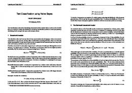
Fig. 1. The robot with whisker attachment. An iRobot Roomba vacuum cleaner was used as a platform for the experiments. The whisker was mounted on the front of the robot, angled down to make constant contact with the floor.

orthogonal displacement angles (X and Y ) of the magnet from its resting position above the sensor. An iRobot Roomba vacuum cleaner (iRobot, 8 Crosby Drive, Bedford, MA 01730) was chosen as the platform for these experiments (Fig. 1). This robot was ideal for the task as it could also be a candidate system for any behavioral output from the texture classification. The whisker was mounted on the front of the robot using epoxy resin, directed at a 45 degree azimuth from the forwards direction of travel and with a slight downwards elevation sufficient to make constant contact with the floor during movement. Thus the whisker transduced a constant stream of deflection information as the robot moved over the floor. Four surfaces were chosen for classification: two carpets of different roughnesses, a tarmac surface and a vinyl surface. These surfaces were chosen because they were appropriately generic for a real world experiment and they provided a range of surface types that were sufficiently similar to make classification difficult. Two primary behavioral conditions were chosen with the robot moving either anticlockwise only, or clockwise only. To demonstrate the difficulty of classification without knowledge of the robot motion, data were also recorded for each surface during the Roomba’s ‘spot’ cleaning programme, which consisted of a series of (externally) unpredictable clockwise, anticlockwise and forward motions. As the robot moved the whiskers were swept across the floor. Any deflections of the whisker were transmitted through the hall effect sensors through a LabJack UE9 USB data acquisition card (www.labjack.com) at a rate of 2kHz for each of the X- and Y -directions. This data was sent to a computer through the BRAHMS middle-

1) Quantized time series: The data are discrete time series of the sensor voltages produced by deflection of the artificial whisker attached to the robot. As this sensor measures both the horizontal and vertical deflections of the whisker, at each sample time there are two distinct sensor voltages x and y associated with these deflections. These voltages are measured at times ti = (i − 1)/fs , where i runs from one to the number of samples n and fs is the sampling frequency. For analysis, it will be convenient to quantize the time series values xi into discrete values. Suppose that all signals under consideration vary between minimum xmin and maximum xmax values, with range ∆x = xmax − xmin . This range is binned into N equal-width intervals, where x is in the qth bin if q q−1 ∆x ≤ x < xmin + ∆x , (1) xmin + N N and if q = N the upper bound also includes xmax . The continuous-valued time series x1 , · · · , xn then becomes a discrete-valued time series q1 , · · · , qn with each qi an integer between one and N . In a similar way, a discrete-valued time series w1 , · · · , wn can be constructed for the samples yi associated with the vertical whisker deflection. Quantization intervals of width 10mV were used here, compared with an approximate 3V spread of sensor measurements. 2) Measurement distributions: The classifier examined here relies on using the probability distributions of the individual time series values, calculated from the empirical frequency with which each measurement value occurs in example (training) data of each texture. If nq is the total number of times that the value q occurs in the quantized time series, then the normalized frequency is pq = nq /n. As PN q=1 nq equals the total number of samples n, the sum of all normalized frequencies equals one and can be interpreted as a probability distribution. Denoting the four textures by T1 , · · · , T4 (for rough carpet, smooth carpet, tarmac and vinyl flooring, respectively), the conditional probability of a quantized measurement q from the texture Tl is nq (Tl ) . (2) n Here the probability distribution for the sensor measurements, P (x|Tl ), is considered to represent the probability of a measurement x being in the interval q(x) = q given it is from the texture Tl . In practice, it was necessary to smooth the normalized frequencies nq to correct for sampling bias in the training data. Without this smoothing, the few samples in the tails of the distributions can lead to large errors in estimating the probabilities, which deteriorates the performance of the classifier. All inferred conditional probabilities were thus P (x|Tl ) ≡ P (q(x)|Tl ) =

Fig. 2. Example data for four textures. The above data for the four floor surface textures was collected in eight trials each of length sixteen seconds, with the four initial trials for clockwise motion and the four final trials for anticlockwise motion.

convolved with a Gaussian smoother of width σ = 100mV (10 quantized intervals), which improved classification performance while smoothing on a relatively small scale compared to the overall spread of data. 3) Bayes classifier (single measurement): The method used here is based on: (a) Supposing the conditional probabilities of the measurements P (x|Tl ) are known from estimating them on training data of all textures. (b) Then, given a measurement x, finding for the most probable texture from which it arose. This method compares the conditional (posterior) probabilities P (Tl |x) for each texture given a measurement x, which are related to the above estimated conditional probabilities by Bayes Theorem, P (x|Tl )P (Tl ) P (Tl |x) = , P (x)

(3)

where P (Tl ) are the (prior) probabilities of having a particular texture, P (x) are the (marginal) probabilities of measuring x given no information about the textures. The conditional probability P (x|Tl ) is now considered a likelihood function. The classifier finds which texture T has maximum a posteriori (MAP) probability given a measurement x. By Eq. 3, T = arg max P (Tl |x) = arg max Tl

Tl

P (x|Tl )P (Tl ) , P (x)

The following arguments assume there is no prior information about which texture is being measured, so that the priors P (Tl ) are all equal and can be ignored when evaluating arg max over the textures. Moreover, since the marginals P (x) are independent of the textures they can also be ignored in the arg max. Finally, it will be convenient to use the logarithm of the posterior probability, and since log(x) (monotonically) increases with x it also does not affect arg max. Putting these arguments together, the texture classification in Eq. 4 is equivalent to finding T = arg max log P (x|Tl ),

(5)

Tl

which is just the maximum over the log-likelihoods determined from the training data given a new measurement x. 4) Naive Bayes classifier (multiple measurements): A potentially more reliable method for classifying textures is to make the decision over many time samples rather than a single value. The arguments in the previous section are unaffected if the single measurement x is replaced by a series of values. Then the equal-prior Bayes texture classification from Eq. 5 becomes T = arg max log P (xns , · · · , xnf |Tl ),

(6)

Tl

(4)

where arg max denotes the argument of the maximum, namely the texture for which P (Tl |x) is maximal.

where ns and nf are the start and finish of the window. An important simplification occurs if the measurements are assumed independent at each time t(i) across the window. Then the overall conditional probability of a series of

Fig. 3. Conditional probabilities of texture measurements. The conditional probabilities were calculated from the empirical frequencies with which the measurement values occur in training data for each of the four textures. Each distribution has been smoothed to reduce sampling bias. Data from the X-sensor (panel A) and Y -sensor (panel B) were considered separately.

347 bins of width 10mV, and the measurements quantized into these intervals (Methods, Eq. 1). The number of measurement values within each bin was then totalled to estimate the conditional probabilities of sensor voltage values for the four textures (Methods, Eq. 2). The resulting probability distribution for each texture is shown in Fig. 3A for the X-sensor and Fig. 3B for the Y -sensor. Notice that the X-sensor probabilities are single peaked, with the means and variances roughly compatible with a visual inspection of the measurements in Fig. 2A,C,E,G. On the other hand, the Y -sensor probabilities have more complicated shapes with two or more peaks. This distribution shape is caused by systematic differences in the response of the Y -sensor to clockwise and anticlockwise motion, as is also visible in Fig. 2. B. Texture classification on X- and Y -sensor validation data

measurements given a texture factorizes into a product of conditional probabilities for each individual measurement P (xns , · · · , xnf |Tl ) = P (xns |Tl ) × · · · × P (xnf |Tl ). (7) Consequently, the classification in Eq. 6 can be rewritten as T = arg max Tl

nf X

log P (xi |Tl ),

(8)

i=ns

Thus the most probable texture is found from the argument of the maximum over the summed log-likelihoods for the series of measurements. 5) Combined X- and Y -sensor classification: Rather than classifying the X- and Y -sensor data individually, it is possible to make a joint classification using both sensors together. Considering the two sensors to take independent measurements, then the overall conditional probabilities for two measurements also factorize into a product of the individual X- and Y -sensor conditional probabilities P (x, y|Tl ) = P (x|Tl )P (y|Tl ),

Given data from an unknown texture, the conditional probability distributions plotted in Fig. 3 can be used as a basis of a classification of which texture is most probable for this data. For validation, the data was separated into discrete segments of fixed temporal window size over which the texture is determined. In general the first half of each trial was used for training and the second half for (holdout) validation, which seemed natural in relation to how a robot or animal might be taught and also allowed the training data to include data correlated beyond the window size. Then the

(9)

Then the classification rule in Eq. 8 can be rewritten as T = arg max Tl

nf X

log P (xi |Tl ) + log P (yi |Tl ).

(10)

i=ns

Thus the most probable texture is found from the argument of the maximum over the summed log-likelihoods for the individual sensor measurements. III. R ESULTS A. Probability distributions from the training data Training data from the four clockwise and four anticlockwise trials (Fig. 2) was pooled to determine the probability distributions for the measured X- and Y -sensor voltages. The initial 8 seconds of each trial was used for training data, and the final 8 seconds of each trial saved for later (holdout) validation of the classification algorithms. The X- and Y -sensor training data was found to vary between 1.36V and 4.83V. This range was separated into

Fig. 4. Hit rates of correct texture identification. The percentage of correct classifications was evaluated over validation data of the four textures. Each hit rate is shown as a function of window size over which the classification was made. Data from the X-sensor (panel A) and Y -sensor (panel B) were considered separately, followed by combining the X and Y measurements in a single classifier (panel C). The single and dual sensor classifications were then compared by their mean hit rates (panel D)

TABLE I C LASSIFICATION OF X - SENSOR VALIDATION DATA (0.5 S WINDOW ). M EAN HIT RATE = 79% Validation data Rough carpet Smooth carpet Tarmac Vinyl

Rough carpet 52% 18% 10% 1%

Smooth carpet 22% 79.5% 5.5% 0%

Tarmac 26% 2.5% 84.5% 0%

Vinyl 0% 0% 0% 99%

TABLE II C LASSIFICATION OF Y - SENSOR VALIDATION DATA (0.5 S WINDOW ). M EAN HIT RATE = 82% Validation data Rough carpet Smooth carpet Tarmac Vinyl

Rough carpet 82.5% 8% 1% 2.5%

Smooth carpet 8.5% 72.5% 19% 0%

Tarmac 1% 19.5% 77% 2.5%

Vinyl 8% 0% 3% 95%

TABLE III C LASSIFICATION OF X & Y - SENSOR VALIDATION DATA (0.5 S WINDOW ). M EAN HIT RATE = 92% Validation data Rough carpet Smooth carpet Tarmac Vinyl

Rough carpet 90% 8% 0% 2.5%

Smooth carpet 8% 90.5% 9.5% 0%

Tarmac 3% 1.5% 90.5% 0%

Vinyl 0% 0% 0% 97.5%

naive Bayes classifier (Methods, Eq. 8) considered the loglikelihood values for the four candidate textures from the conditional probability distributions at the same measurement value in the training data. These log-likelihoods were summed across the window for each of the four textures, and the maximum one gave the classified texture. The proportion of correct classifications, or hits, across validation data for each of the four textures is shown in Fig. 4A for the X-sensor and Fig. 4B for the Y -sensor. The classification was clearly a success, with the data from both sensors reaching a good mean hit rate of about 80%. Even though some hit rates improved and some worsened with increasing window size, the mean hit rate improved steadily across the range of window sizes shown (Fig. 4D). This mean hit rate improved substantially as the window size was increased from 0.5ms (single sample) to 100ms, and then modest gains occurred thereafter. Notice also that the two sensors had problems with different textures: the X-sensor classifier was most mistaken for rough carpet, while the Y sensor classifier was worst on smooth carpet. Details of the texture classification and misclassification are shown in Table I for the X-sensor data and Table II for the Y -sensor data at a fixed window size of 0.5 seconds. The diagonals of each table are the percentages of correct classifications over the validation data for each texture. Consistent with Fig. 4A,B, vinyl was excellently classified (> 90%) for either sensor, while rough carpet was the most difficult to classify with the X-sensor (∼ 50%) but well classified (∼ 80%) with the Y -sensor. The mean hit rate

was calculated over the diagonal of the table, and was about 80% for either sensor. The off-diagonal elements represent how often each texture is misclassified as another texture and can be thought of the degree of confusion. For example, the X-sensor classification confuses rough carpet with tarmac 26% of the time and almost never confuses anything with vinyl. The confusion between rough carpet and tarmac is consistent with visual inspections of the data (c.f. Figs 2A and 2C) and the probability distributions (Fig. 3A), both of which are quite similar by eye. To illustrate when the classifiers make mistakes, Fig. 5 shows the texture classification applied to Y -sensor validation data for the four textures. Hits are shown on the plot by coloring the data black and misses in gray. It is interesting that the instances when a texture was misclassified often coincide with artifacts in the data. For example, the rough and smooth carpets were mainly misclassified on dead-zones and the vinyl texture is misclassified on jumps. In a sense, therefore, the classification algorithm is not really making mistakes, but is instead identifying correctly where the data does not look like a typical example of that texture. C. Improved classification by combining X- and Y -data Rather than using validation data from the X- and Y sensors individually, it is possible to perform a classification using both sets of data together (Methods, Eq. 10). Because more evidence is used in the classification, the combined

Fig. 5. Examples of misclassification. The panels show the performance of the classification over a 0.5 second window applied to Y -sensor validation data of the four textures. Hits are shown in black and misses in gray.

TABLE IV C LASSIFICATION OF X & Y - SENSOR VALIDATION DATA (0.5 S WINDOW ). A RTIFICIAL TRAINING DATA ; NATURAL VALIDATION DATA . M EAN HIT RATE = 68.0% Validation data Rough carpet Smooth carpet Tarmac Vinyl

Rough carpet 67% 2% 3% 23%

Smooth carpet 32% 97% 9.5% 9.5%

Tarmac 1% 1% 87.5% 47%

Vinyl 0% 0% 0% 20.5%

TABLE V C LASSIFICATION OF X & Y - SENSOR VALIDATION DATA (0.5 S WINDOW ). NATURAL TRAINING DATA ; NATURAL VALIDATION DATA . M EAN HIT RATE = 81% Validation data Rough carpet Smooth carpet Tarmac Vinyl

Rough carpet 88% 8% 6% 7%

Smooth carpet 12% 91.5% 2.5% 0%

Tarmac 0.5% 0.5% 91.5% 40%

Vinyl 0% 0% 0% 53%

X- and Y -sensor classifier should be more accurate. In particular, a main cause of misclassifications of the individual sensor data was when a sensor picked up an artifact such as a dead-zone or jump. Using data from both sensors together gave more chance of receiving reliable information from at least one of the sensors when the signals are hard to discriminate. The hit rate of correct texture identification is shown in Fig. 4C for the combined X- and Y -sensor classifier. The combined classification is clearly a substantial improvement over the results for the individual sensors in Figs 4A,B, with all textures reaching an excellent correct identification of about 90% for window sizes of 0.5 seconds or more. The classification of vinyl has suffered slightly compared to that by just the X-sensor, but this is more than compensated by the significant gains in classifying the other textures. These improvements can be seen more clearly in a comparison of the mean hit rate for the X-sensor, Y -sensor and combined XY -sensor classifier in Fig. 4D: the combined sensor classification reaches a mean hit rate of about 90% compared to about 80% for the individual sensors. Details of the texture classification and misclassification for the combined XY -sensor classification are shown in Table III for a window size of 0.5 seconds. The percentages of correct classifications are shown down the diagonal, and are all 90% or greater. The percentages of misclassifications are shown by the off-diagonal elements. Roughly speaking, if the individual X- and Y -sensor classifiers confuse two textures, then these are mistaken to a lesser-degree by the combined XY -sensor classification.

validation). A more difficult task is whether the texture classification is still successful on ‘natural’ motion, taken from the Roomba’s internal programme of a series of (externally) unpredictable clockwise, anticlockwise, stationary and forward motions. The first classification was for artificial training data and natural validation data (results in Table IV), applying the same combined XY -sensor classifier as in the previous section. The classifier performed excellently on smooth carpet (97%) and tarmac (87.5%), adequately on rough carpet (57%) and terribly on vinyl flooring (20.5%). The mean hit rate (68%) is shifted down relative to that for the artificial validation data (Table III, 92%), mainly by the poor performance on vinyl. Curiously, none of the other textures are confused with vinyl, even though it is frequently confused with rough carpet (23%) and tarmac (47%). Natural training and natural validation data were then considered, using training data from the first half of each natural trial and validation data from the second half. The results of the combined XY -sensor classification text are shown in Table V. The classification was now excellent (∼ 90%) on all textures except for a moderate performance on vinyl (53%). Therefore, other than for vinyl, the classification generalized well from artificial to natural data, and even performed adequately if trained on the artificial data and applied to the natural data. Unfortunately, vinyl was not well-recognized on natural data, which was a surprise considering that it was most easily classified for the artificial motion. However, closer inspection of the natural vinyl data revealed a systematic difference between the initial and final four trials of the X sensor data (Fig. 6A) that was absent in the artificial data (Fig. 2G). This difference explains the poor performance (20.5%) when classifying vinyl using artificial training and natural validation data, as the absence of this important feature in the training data made recognition of the natural data impossible. The moderate performance (53%) on natural training and validation data is more difficult to explain, and could relate to a limitation of the naive Bayes classifier, such

D. Application to ‘natural’ data Thus far the classification algorithm has been both trained on and validated against data from artificial, stereotyped clockwise or anticlockwise robot motion (with the first half of each trial used for training and the second half for

Fig. 6. Natural data for the vinyl texture. The data was collected in eight trials each of length sixteen seconds, where the robot performed ‘natural’ motion according to its internal program.

as not using the clearly visible temporal correlations in the natural vinyl data (Fig. 6) or a correlation between the X and Y sensor measurements. IV. D ISCUSSION To examine the underlying processes involved in sensing surface textures with whiskers, data from an artificial whisker attached to a moving robot was used for testing possible classification algorithms. This data was previously analyzed using a template matching method on the whisker vibration power spectrum [1]. Here a naive Bayes classifier was used on the raw vibration signal: this method estimates the most probable texture to have produced a series of measurements, given estimated likelihoods for single measurements from training data of the textures. The naivety refers to using only the likelihood from single measurements, which ignores any temporal structure in the data. Our reason for using this classifier was that it relates to proposed mechanisms for neural decision making [2], [13]–[15]. The naive Bayes classifier gave excellent results on data from four different textures (rough carpet, smooth carpet, tarmac, vinyl flooring). For stereotyped clockwise and anticlockwise motion, the algorithm could reliably recognize textures with a mean hit rate of about 80% using single stream data from either the X- or Y -sensor whisker deflection. If both X- and Y -sensor data streams were considered together, the mean hit rate improved to a very impressive 90%. It was important that enough data was being used to make a decision, with temporal window sizes of about 500ms being necessary to give these hit rates. Furthermore, the times when incorrect decisions were made tended to coincide with artifacts such as dead zones or jumps, consistent with the algorithm then identifying correctly where the data does not look like the texture on which it has been trained. The classifier was also applied to ‘natural’ motion, taken from a series of (externally unpredictable) clockwise, anticlockwise, stationary and forward motions. Although there were now problems with vinyl flooring, the classifier could still recognize the other three textures with approximately 90% success. A. Comparison with the spectral template-based classifier The robot whisker data was previously examined in a study that used a spectral template-based classifier [1]. Spectral classifiers characterize data from the profile of their power spectra. In the previous study, training data of each texture was separated into 400ms segments, from which a template was estimated from the mean power spectrum for each texture (Fig. 7, Ref. [1]). The performance of the template matching was then analyzed on validation data of each texture. First, the power spectrum over each 400ms segment of validation data was found, followed by a determination of the mean square error from each of the texture templates, which then classified the data segment according to the template with the lowest error.

Theoretically, there are two (related) differences between the spectral method and our use of the naive Bayes classifier: (a) The naive Bayes classifier was applied to the raw whisker deflection data, whereas the spectral classifier uses the frequency spectrum of the whisker signal captured by the power spectra; (b) The naive Bayes classifier does not use any information about statistical dependance of the signals at different times, whereas the spectral classifier uses only information about the statistical dependance, represented by the power spectrum. Hence, we view the two methods as complementary approaches, since each uses a quite different component of the information available from the whisker. This is important because both methods could in principle be combined together to give a more reliable classifier than either on its own. The differences in performance between the two classifiers can be seen by direct comparison. For stereotyped texture data from clockwise or anti-clockwise motion, the spectral classifier achieved an overall mean hit rate of 72% (clockwise) and 64% (anticlockwise) using a data from just the Xsensor, whereas naive Bayes achieved about 80% over both motions with either the X- or Y -sensor. Therefore the naive Bayes classifier does seem to be moderately more reliable when the hit rates over all textures are averaged. Note though that the two classifiers have problems with different textures. For X-sensor data, the spectral classifier had most difficulty with smooth carpet (33% and 54% hit rates; clockwise/anticlockwise) and performed well on rough carpet (78% and 64%) while the naive Bayes classifier performed well on smooth carpet (79.5%) and found rough carpet most problematic (52% hit rate). Moreover, for natural data, the spectral classifier performed well on all textures (hit rates 60-77.5%) except smooth carpet (11%), while the naive Bayes classifier (both sensors) performed well on all textures (hit rates 88-91.5%) except vinyl (53%). This behavior is consistent with the two methods being complementary in their performance in addition to their theoretical basis. B. Relation to biological decision making Our use of the naive Bayes classier in the present study is motivated by a proposal for the neural computations that underlie decisions about sensory stimuli. Based upon measurements of neural activity in monkeys performing perceptual decision making (e.g. [12]), Gold and Shadlen suggested that the logarithm of the likelihood ratio (log LR) provides a natural currency for forming a perceptual decision [2]. The likelihood ratio applies only to choices between two alternatives, say H1 and H2 , with a decision rule that given a sequence of measurements x1 , · · · , xn , n X i=1

log LR1,2 (xi ) =

n X i=1

log

P (xi |H1 ) ≷ 0, P (xi |H2 )

(11)

where greater than zero supports hypothesis H1 and less than zero H2 . This decision rule is identical mathematically to the naive Bayes MAP rule in Eq. 8 for two textures. Crucially, both naive Bayes and the log-likelihood ratio are based on

assuming that the measurements xi are independent over time. In this sense, we interpret naive Bayes’ as a direct extension of Gold and Shadlen’s proposal to the situation with three or more alternatives. Such a mechanism is known more generally as evidence accumulation or Bayesian integration and has formed the basis for a number of proposals for neural decision making [13]–[15] Therefore we see the present whiskered robot study as an initial stage in clarifying tactile decision making processes in rodents. We showed that a simple, texture classification algorithm, which is closely related to a number of proposals for perceptual decision making, is an excellent classifier of textures for a robot moving in (its) natural environment. This suggests a functional hypothesis for tactile decision-making in rodents based on a similar evidence accumulation strategy. The log-likelihoods could be stored from previous experience of the textures, and then a decision reached on a new stream of sensory experience by accumulating evidence for each of these texture ‘memories’. A complementary step to investigate such a proposal would be to examine electrophysiological recordings from barrel cortex to see whether whisker vibrations can also be distinguished with similar computational methods. If successful, these studies taken together would give reasonable circumstantial evidence for a related form of decision making in rodents. That being said, a true test of the neural processing could only be achieved by comparing the computational results to the performance of an awake, behaving rat. A behavioral performance that was neither more nor less accurate than that achieved by the classifier on barrel cortex activity would provide strong evidence that the rat uses such a decision making strategy. ACKNOWLEDGMENTS The authors would like to thank members of the Active Touch Laboratory at Sheffield, the Bristol Robotics Laboratory, and the Tactile Perception and Learning Laboratory in SISSA for discussions. This work was supported by EU grants ICEA (IST-027819) and BIOTACT (ICT-215910).

R EFERENCES [1] M. Evans, C. W. Fox, M. J. Pearson and T. J. Prescott, “Spectral Template Based Classification of Robotic Whisker Sensor Signals in a Floor Texture Discrimination Task,” Proc. 10th Conference Towards Autonomous Robotics Systems, Ulster, U.K., Aug. 2009. [2] J. I. Gold and M. N. Shadlen, “Neural computations that underlie decisions about sensory stimuli,” Trends Cogn Sci., vol. 5 (1), pp. 1016, Jan. 2001. [3] G. E. Carvell and D. J. Simons, “Biometric analysis of vibrissal tactile discrimination in the rate,” J Neurosci., vol. 10 (8), pp. 2638–48, 1990. [4] E. Arabzadeh, S. Panzeri, M. E. Diamond, “Whisker vibration information carried by rat barrel cortex neurons,” J Neurosci., vol. 24 (26), pp. 6011-20, Jun. 2004. [5] E. Arabzadeh, S. Panzeri, M. E. Diamond, “Deciphering the spike train of a sensory neuron: counts and temporal patterns in the rat whisker pathway,” J Neurosci., vol. 26 (36), pp. 9216-26, Sep. 2006. [6] M. von Heimendahl, P. M. Itskov, E. Arabzadeh, M. E. Diamond, “Neuronal activity in rat barrel cortex underlying texture discrimination,” PLoS Biol, vol. 5 (11), e. 305, Nov. 2007. [7] A. Lak, E. Arabzadeh, M. E. Diamond, “Enhanced response of neurons in rat somatosensory cortex to stimuli containing temporal noise,” Cereb Cortex., vol. 18 (5), pp. 1085-93, May 2008. [8] A. K. Seth, J. L. McKinstry, G. M. Edelman, and J. L. Krichmar, “Texture discrimination by an autonomous mobile brain-based device with whiskers,” Proc. 2004 IEEE International Conference on Robotics & Automation, New Orleans, LA, April 2004. [9] M. Fend, “Whisker-based texture discrimination on a mobile robot,” In Lecture notes in computer science. Proc. 8th European conference on artificial life (ECAL). Berlin: Springer. [10] C. W. Fox, B. Mitchinson, M. J. Pearson, A. G. Pipe and T. J. Prescott, “Contact type dependency of texture classification in a whiskered mobile robot,” Auton Robot, vol. 26, pp. 223239, 2009. [11] J. Hipp, E. Arabzadeh, E. Zorzin, J. Conradt, C. Kayser, M. E. Diamond, P. K onig “Texture signals in whisker vibrations,” Neurophysiol. vol. 5 (3), pp. 1792-9, Mar 2006. [12] J. I. Gold and M. N. Shadlen, “Representation of a perceptual decision in developing oculomotor commands,” Nature, vol. 404, pp. 390-394, 2000. [13] J. B Tenenbaum and T. L Griffiths, “Generalization, similarity, and Bayesian inference,” Behavioral and Brain Sciences, vol. 4 (24), pp. 629-640, 2002. [14] K. Kording, “Decision theory: what should the nervous system do?,” Science, vol. 318, pp. 606-610, 2007. [15] R. Bogacz and K. Gurney, “The basal ganglia and cortex implement optimal decision making between alternative actions,” Neural computation, vol. 19 (2), pp. 442-477, 2007. [16] D. J. Hand and K. Yu, “Idiot’s Bayes - not so stupid after all?,” International Statistical Review, vol. 69 (3), pp. 385399, 2001. [17] I. Rish, “An empirical study of the naive Bayes classifier,” Proc. 17th International Joint Conference on Artificial Intelligence (IJCAI), Seattle, U.S., Aug. 2001.