Naming Proofs in Classical Propositional Logic - LIX-polytechnique

January 31, 2005 — Final version, appearing in proceedings of TLCA’05.

Naming Proofs in Classical Propositional Logic Fran¸cois Lamarche

Lutz Straßburger

LORIA & INRIA-Lorraine Projet Calligramme 615, rue du Jardin Botanique 54602 Villers-l`es-Nancy — France http://www.loria.fr/~lamarche

Universit¨ at des Saarlandes Informatik — Programmiersysteme Postfach 15 11 50 66041 Saarbr¨ ucken — Germany http://www.ps.uni-sb.de/~lutz

Abstract. We present a theory of proof denotations in classical propositional logic. The abstract definition is in terms of a semiring of weights, and two concrete instances are explored. With the Boolean semiring we get a theory of classical proof nets, with a geometric correctness criterion, a sequentialization theorem, and a strongly normalizing cut-elimination procedure. This gives us a “Boolean” category, which is not a poset. With the semiring of natural numbers, we obtain a sound semantics for classical logic, in which fewer proofs are identified. Though a “real” sequentialization theorem is missing, these proof nets have a grip on complexity issues. In both cases the cut elimination procedure is closely related to its equivalent in the calculus of structures.

1

Introduction

Finding a good way of naming proofs in classical logic—a good theory of proof terms, or proof nets, or whatever—is a notoriously difficult question, and the literature about it is already quite large, and still increasing. Other logics have been helped enormously by the presence of good semantics, where by semantics we mean mathematical objects that have an independent existence from syntax. Linear logic was found through the observation of the category of coherence spaces and linear maps. For intuitionistic logic, it has been obvious for a long time that all it takes to give an interpretation of formulas and proofs ` a la Brouwer-Heyting-Kolmogorov-Curry-Howard is a bi-cartesian closed category. . . and cartesian closed categories abound in nature. But if we try to extend naively these semantics to classical logic, it is wellknown that everything collapses to a poset (a Boolean algebra, naturally) and we are back to the old semantics of provability. Clearly something has to be weakened, if we ever want classical logic to have a meaning beyond syntax. Very recently, it was found [17] that a class of algebras from geometry permits relevant interpretations of classical proofs; in addition proposals for abstract categorical frameworks has been made; the one in [10, 11] is based on the proof nets of [24] (which avoids poset collapse is by not identifying arrow composition with cutelimination), and the one in [9] extends the tradition of “coherence” results in category theory, which predates linear logic by decades.

Let us describe succinctly the view when this problem is approached from the other end, that of syntax. We use the sequent calculus as our main proof paradigm, but what we say is presented so as to apply to natural deduction as well. It is well known that problems begin when a proof contains redundancies and has to be normalized. Let us represent this situation in the following manner ?? ? ??π1  ???π2  ? ? cut

¯ ∆ ` A,

` Γ, A

.

` Γ, ∆

Here, we use one-sided notation for sequents for the sake of generality, and an expression like A could be a formula with some polarity information added, instead of just a formula. The π1 and π2 represent the proofs that led to the sequents: they could be sequent calculus trees, proof terms or proof nets. Similarly, the expression A¯ is a formal negation for A; this notation could be used for instance in a natural deduction context like the λµ-calculus [22], where the “cut” inference above would just be a substitution of a term into another, the negated A¯ meaning that it is on the side of the input/premises/λ-variables. But nonetheless the following have for a long time been identified as Desirable Features: 1. A¯ is the logical negation of A, 2. A¯ is structurally equivalent (isomorphic) to A. These additional symmetries simplify life enormously, allowing things like structural de Morgan duals. The second feature will not happen, for example, when negation is an introduced symbol, as in the case for two-sided sequent calculi or the λµ-calculus (for which the first feature does not hold either). The problem of cut-elimination (or normalization) is encapsulated in two cases, called weakening-weakening and contraction-contraction in [12], which hereafters will be written as weak-weak and cont-cont: ?? ?? ?? ?? ??π2  ??π1  ??π2  ??π1  ? ? ? ? weak cut

`Γ

` Γ, A

weak ` Γ, ∆

`∆ ¯ ∆ ` A,

cont and

` Γ, A, A

cut

` Γ, A

cont ` Γ, ∆

¯ A, ¯ ∆ ` A, ¯ ` A, ∆

.

It is well known [13, 12] that both reductions cannot be achieved without choosing a side, and that the outcome is very much dependent on that choice. The most standard way to resolve these dilemmas is to introduce asymmetry in the system (if it is not already there), by the means of polarity information on the formulas, and using this to dictate the choices. Historically, the first approaches to polarization were closely aligned on the premiss/conclusion duality we have mentioned. One reason for this is that they were derived from doublenegation style translations of classical logic into intuitionistic logic. If a classical proof can be turned into an intuitionistic one, then in every sequent in the history of that proof there will be a special formula: the conclusion of the corresponding intuitionistic sequent. This is what is done, for example, mutatis mutandis, in the λµ-calculus. 2

This left-right asymmetry is also at the bottom of Coquand’s game semantics [6], where it translates as the two players. In [12] Girard presented System LC, where the sequents have at most one special formula. Not only are there both positive and negative formulas—this time an arbitrary number of each—but in addition there is a stoup, which is either empty or contains one formula, which has to be positive. Then when a choice has to be made at normalization time, the presence or absence of the positive formula in the stoup is used in addition to the polarity information. This calculus has very nice properties; in particular both Desirable Features above are present. System LC was discovered by the means of a translation into a bi-cartesian closed category C , but something much weaker can be used. Our story would be over if everything had been solved by that approach; but semantic cut-elimination (composition of denotations of proofs) is not associative here in general; this is shown by a case analysis on the polarities. Thus normal forms are still dependent somehow on the history of the proof’s construction. Viewed from another angle this says that the category C cannot inherently be a model for classical logic (composition in categories is associative. . . ), it is more a vehicle for a translation. This direction of research has nonetheless been extremely fruitful. It has given a systematic analysis of translations of classical logic into linear logic [7]. Moreover LC’s approach to polarities was extended to the formulation of polarized logic LLP [19]. It has the advantage of a much simpler theory of proof nets (e.g., for boxes) and produces particularly perspicuous translations of more traditional logics. This new proof net syntax has been used to represent proofs in LC [19] and the λµ-calculus [20]. Let us go back to the weak-weak and cont-cont problems. It is well-known (e.g., [8]) that one way of solving weak-weak is to permit the system to have a mix rule. As for the cont-cont problem, the proof formalism of the calculus of structures [15, 2] has permitted the emergence of a novel solution: through the use of deep inference a proof can always be transformed into one whose only contractions are made on constants and atomic formulas. In this paper we exploit these two ideas to construct two systems of proof denotations for classical logic, which are at the border of syntax and semantics, and which possess both Desirable Features as well as one of the main features of proof nets, since a proof of a formula is represented as a graph structure on on its set of atoms, the edges being directly related to the axioms of a corresponding sequent proof. But other standard features of non-multiplicative proof nets (boxes and explicit contraction links) are absent—we hasten to say that it has been shown in [16] that multiplicative-additive linear logic can be presented in the same manner as we do, strictly as additional structure on the atomic formulas, without explicit contractions. The most important of the two systems here is the first one; it benefits from a full completeness theorem—in other words, a correctness criterion and a sequentialization theorem—and so it can be used directly to represent proofs, without recourse to other syntactical formalisms. Moreover strong normalization holds, in the most general sense. The other system conveys both more and less information at the same time: the number of 3

times an axiom link is used in a proof is counted, but since we do not have (as of yet) a sequentialization theorem, it is closer to a semantics, in particular to the Geometry of Interaction. Issues of normalization are much more delicate in this latter system, but it has a definite interest from the point of view of complexity. One important aspect of the first system is that it seems to contradict some widely held ideas about proof terms: it is a collection of term-like objects (nets) with a notion of composition (cut) and for which we have a strong normalization theorem. But it cannot be said to come from the Curry-Howard tradition. In other words the cut-elimination procedure cannot be used as a paradigm of computation. There is more research to be done on this issue. It could be that polarities also introduce another distinction: that between data and program. Remarkably the idea of using axiom links to capture a proof in classical logic (including the correctness criterion!) has been around since Andrews’ paper of 1976 [1], and his use of the term “essence of a proof” clearly shows that he understood what was at stake. But since he was working on proof search, he never explored the possibility of composing these “essences”. The idea of keeping all axiom links that appear in a sequent proof is already present in Buss’ logical flow graphs [3, 4].

2

Cut free proof nets for classical propositional logic

Let A = {a, b, . . . } be an arbitrary set of atoms, and let A¯ = {¯ a, ¯b, . . . } the set of their duals. The set of CL-formulas is defined as follows: F ::= A | A¯ | t | f | F ∧ F | F ∨ F . We will use A, B, . . . to denote formulas. The elements of the set {t, f } are called constants. A formula in which no constants appear is called a CL0 -formula. Sequents, denoted by Γ , ∆, . . . , are finite lists of formulas, separated by comma. In the following, we will consider formulas as binary trees (and sequents as forests), whose leaves are decorated by elements of A ∪ A¯ ∪ {t, f }, and whose inner nodes are decorated by ∧ or ∨. Given a formula A or a sequent Γ , we write L (A) or L (Γ ), respectively, to denote its set of leaves. For defining proof nets, we start with a commutative semiring of weights (W, 0, 1, +, ·). That is, (W, 0, +) is a commutative monoid structure, (W, 1, ·) is another commutative monoid structure, and we have the usual distributivity laws x·(y +z) = (x·y)+(x·z) and 0·x = 0. This abstraction layer is just there to ensure a uniform treatment for the two cases that we will encounter in practice, namely W = N (the semiring of the natural numbers with the usual operations), and W = B = {0, 1} (the Boolean semiring, where addition is disjunction, i.e., 1 + 1 = 1, and multiplication is conjunction). There are two additional algebraic properties that we will need: v + w = 0 implies v = w = 0 (1) v · w = 0 implies either v = 0 or w = 0 . (2) These are obviously true in both concrete cases. No other structure or property on B and N is needed, and thus other choices for W can be made. They all give sound semantics, but completeness (or sequentialization) is another matter. 4

2.1 Definition Given W and a sequent Γ , a W -linking for Γ is a function P : L (Γ ) × L (Γ ) → W which is symmetrical (i.e., P (x, y) = P (y, x) always), and such that whenever P (x, y) 6= 0 for two leaves, then one of the following three cases holds: 0. one of x and y is decorated by an atom a and the other by its dual a ¯, 1. x = y and it is decorated by t, or 2. one of x and y is decorated by t and the other by f . A W -pre-proof-net 1 (or shortly W -prenet) consists of a sequent Γ and a linking P for it. It will be denoted by P B Γ . If W = B we say it is a simple pre-proof-net (or shortly simple prenet). In what follows, we will simply say prenet, if no semiring W is specified. If we choose W = B, a linking is just an ordinary, undirected graph structure on L (Γ ), with an edge between x and y when P (x, y) = 1. An example is .......................................... ............................ ........................................................................................................................ . . . . . ....... ... .. ..... ... .... ... ....... .......... ............. .... .......... ..... .. ¯ ¯b 2 a a¯ 2 b b 2 a a¯ 2 b ∧



∧



∧



∧

(3)



To save space that example can also be written as _ _ _ _ _ _ { ¯b1 b5 , ¯b1 b8 , ¯b4 b5 , ¯b4 b8 , a2 a ¯3 , a6 a ¯7 } B ¯b1 ∧ a2 , a ¯3 ∧ ¯b4 , b5 ∧ a6 , a ¯ 7 ∧ b8 , where the set of linked pairs is written explicitly in front of the sequent. Here we use the indices only to distinguish different atom occurrences (i.e., a3 and a6 are not different atoms but different occurrences of the same atom a). For more general cases of W , we can consider the edges to be decorated with elements of W \ {0}. When P (x, y) 6= 0 we say that x and y are linked. Here is an example of an N-prenet: 2 3 _ _ _ _ { t1 t1 , a4 a ¯5 , t7 t7 , t7 f8 } B t1 ∨ (a2 ∧ t3 ), (a4 ∨ (¯ a5 ∨ f6 )) ∧ (t7 ∨ f8 ) .

(4)

As before, no link means that the value is 0. Furthermore, we use the convention that a link without value means that the value of the linking is 1. When drawing N-prenets as graphs (i.e., the sequent forest plus linking), we will draw n links between two leaves x and y, if P (x, y) = n. Although this might be a little cumbersome, we find it more intuitive. Example (4) is then written as ............ ...................... .... ... t- a 2 t - -- ∧ ∨



.......... ................. ..................... a- a ¯2

f

............. .......... .t 2 f

- -- ∨ ∨



∨ OOO

OO

.

(5)

∧

Now for some more notation: let P B Γ be a prenet and L ⊆ L (Γ ) an arbitrary subset of leaves. There is always a P |L : L × L → W which is obtained by restricting P on the smaller domain. But L also determines a subforest Γ |L 1

What we call pre-proof-net is in the literature often called a proof structure.

5

of Γ , in the manner that all elements of L are leaves of Γ |L , and an inner node s of Γ is in Γ |L if one or two of its children is in Γ |L . Thus Γ |L is something a bit more general than a “subsequent” or “sequent of subformulas”, since some of the connectors are allowed to be unary, although still labeled by ∧ and ∨. Let Γ 0 = Γ |L . Then not only is Γ 0 determined by L, but the converse is also true: L = L (Γ 0 ). We will say that P |L B Γ 0 is a sub-prenet of P B Γ , although it is not strictu sensu a prenet. Since this sub-prenet is entirely determined by Γ 0 , we can also write it as P |Γ 0 B Γ 0 without mentioning L any further. On the set of W -linkings we define the following operations. Let P : L × L → W and Q : M × M → W be two W -linkings. – If L = M we define the sum P + Q to be the pointwise sum (P + Q)(x, y) = P (x, y) + Q(x, y). When W = B this is just the union of the two graphs. – If L ⊆ M we define the extension P ↑M of P to M as the binary function on M which is equal to P (x, y) when both x and y are in L and zero elsewhere. Most of the times we will write P ↑M simply as P . – If L and M are disjoint, we define the disjoint sum P ⊕ Q on the disjoint union2 L ] M as P ⊕ Q = P ↑L]M +Q ↑L]M . 2.2 Definition A conjunctive resolution of a prenet P B Γ is a sub-prenet P |Γ 0 B Γ 0 where Γ 0 has been obtained by deleting one child subformula for every conjunction node of Γ (i.e., in P |Γ 0 B Γ 0 every ∧-node is unary). 2.3 Definition A W -prenet P B Γ is said to be correct if for every one of its conjunctive resolutions P |Γ 0 B Γ 0 the W -linking P |Γ 0 is not the zero function. A W -proof-net (or shortly W -net) is a correct W -prenet. A correct B-prenet is also called a simple net. Both examples shown so far are correct: (3) is a B-net as well as an N-net; (5) is an N-net. Notice that the definition of correctness does not take the exact values of the weights into account, only the presence (P (x, y) 6= 0) or absence (P (x, y) = 0) of a link. Notice also that correctness is a monotone property because of Axiom (1): if P B Γ is correct then P + Q B Γ is also correct. The terms “linking” and “resolution”, as well as the B-notation, have been lifted directly from the work on multiplicative additive (MALL) proof nets of [16], and we use them in the same way, for the same reasons. In fact, there is a remarkable similarity between the MALL correctness criterion therein—when restricted to the purely additive case—and ours (which is essentially the same as Andrews’ [1]); this clearly deserves further investigation.

3

Sequentialization

Figure 1 shows how sequent proofs are mapped into prenets. The sequent system we use contains the multiplicative versions of the ∧- and ∨-rules, the usual axioms for identity (reduced to atoms and constants) and truth, as well as the rules of exchange, weakening, contraction, and mix. We call that system CL (for Classical Logic). We use three minor variations: CL0 where the only axiom available is id0 , 2

If L and M are not actually disjoint, we can rename one of the sets to ensure that they are.

6

id0

∨

t1

_ {a a ¯ } B a, a ¯ P B A, B, Γ P B A ∨ B, Γ

weak

P BΓ P B A, Γ

∧

_ {t t} B t

P B Γ, A

Q B B, ∆

P ⊕ Q B Γ, A ∧ B, ∆ cont

P B A, A, Γ 0

P B A, Γ

id2

exch

mix

_ { f t } B f, t P B Γ, A, B, ∆ P B Γ, B, A, ∆

P BΓ

QB∆

P ⊕ Q B Γ, ∆

Fig. 1. Translation of cut free sequent calculus proofs into prenets

involving only atoms, CL1 which allows in addition the axiom t1 , and CL2 which allows all three axioms. In the case of CL0 we consider only CL0 -formulas, and in CL1 and CL2 we consider all CL-formulas. When we write just CL we mean CL2 . There are two rules that are not strictly necessary from the point of view of provability, namely mix and id2 . Thus, although we do not get more tautologies by including these rules in the system, we get more proofs. These new proofs are needed in order to make cut elimination confluent (mix), and get identity proofs in the logic with units (id2 ), thus allowing us to construct a category. It is only one more example of the extreme usefulness of completions in mathematics: adding stuff can make your life simpler. Let us now explain the translation from CLi sequent proofs to prenets. We should have a notion of CLi -prenet for any one of i = 0, 1, 2, and Definition 2.1 has been designed to produce them automatically: a CLi -prenet is one where conditions 0, . . . , i hold in that definition. The construction is done inductively on the size of the proof. In the two rules for disjunction and exchange, nothing happens to the linking. In the case of weakening we apply the extension operation to P . In the mix and ∧ rules we get the linking of the conclusion by forming the disjoint sum of the linkings of the premises. Therefore, the only rule that deserves further explanation is contraction. Consider the two sequents ∆0 = A, Γ and ∆ = A, A, Γ , where ∆ is obtained from ∆0 by duplicating A. Let p : L (∆) → L (∆0 ) be the function that identifies the two occurrences of A. We see in particular that for any leaf x ∈ L (∆0 ), the inverse image p−1 {x} has either one or two elements. Given P B ∆ let us define the linking P 0 for ∆0 as X P 0 (x, y) = P (z, w) . z∈p−1 {x} w∈p−1 {y}

3.1 Theorem (Soundness) Given any W as above, any i ∈ {0, 1, 2} and a sequent proof in CLi , the construction above yields a correct W -prenet. Proof: The proof is an easy induction and will be left to the reader for the time being. Notice that we need Axiom (1) for the contraction rule, but not (2). u t We say a prenet is sequentializable if it can be obtained from a sequent calculus proof via this translation. Theorem 3.1 says that every sequentializable prenet is a net. 7

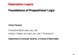
3.2 Theorem (Sequentialization) For any i ∈ {0, 1, 2}, a simple CLi -net (i.e., W = B) is sequentializable in CLi . Proof: We proceed by induction on the size of the sequent (i.e., the number of ∧-nodes, ∨-nodes, and leaves in the sequent forest). Consider a simple net P B ∆. We have the following cases: – If ∆ contains a formula A ∨ B, then we can apply the ∨-rule, and proceed by induction hypothesis. – If ∆ contains a formula A ∧ B, i.e., ∆ = Γ, A ∧ B, then we can form the three simple nets P 0 B Γ, A and P 00 B Γ, B and P B Γ, A, B, where P 0 = P |Γ,A and P 00 = P |Γ,B . All three of them are correct, quite obviously. Therefore, we can apply the induction hypothesis to them. Now we apply the ∧-rule twice to get P 0 ⊕ P 00 ⊕ P B Γ, Γ, Γ, A ∧ B, A ∧ B . To finally get P B Γ, A ∧ B, we only need a sufficient number of contractions (and exchanges). Let us make two remarks about that case: • If P B Γ, A ∧ B contains no link between A and B, i.e., P |A,B = P |A ⊕ P |B , then we do not need the net P B Γ, A, B, and can instead proceed by a single use of the ∧-rule, followed by contractions. • This is the only case where the fact that W = B is needed. – If ∆ = Γ, A, such that P = P |Γ , i.e., the formula A does not take part in the linking P , then we can apply the weakening rule and proceed by induction hypothesis. – The only remaining case is where all formulas in ∆ are atoms, negated atoms, or constants. Then the sequent proof is obtained by a sufficient number of instances of the axioms id0 , t1 , id2 , and the rules cont, exch, and mix. t u Note that the particular sequent system CL is only needed for obtaining the completeness, i.e., sequentialization, of B-nets. For obtaining the soundness result, any sequent system for classical propositional logic (with the identity axiom reduced to atomic form) can be used. Moreover, this is not restricted to sequent calculus. We can also start from resolution proofs (as done in [1]), tableau proofs, Hilbert style proofs, etc. Whereas B-nets only take into account whether a certain axiom link is used in the proof, N-nets also count how often it is used. Therefore, N-nets can be used for investigating certain complexity issues related to the size of proofs, e.g., the exponential blow-up usually related to cut elimination. This is not visible for B-nets, where the size of a proof net is always quadratic in the size of the sequent. It should not come as a surprise that finding a fully complete correctness criterion for N-nets is much harder. One reason is the close connection to the NP vs. co-NP problem [5]. Moreover, there are correct N-nets for which no corresponding sequent proof exists, for example (3) seen as an N-net, but which can be represented in other formalisms, for example the calculus of structures [15, 2]). Because of the conflation of sequents and formulas into a single kind of syntactic expression, we can write the proof that is shown on the left of Figure 2, and whose translation into N-nets is exactly (3)—To save space we did in the figure several steps in one. For example id4 stands for four applications of the identity rule. 8

id4 s4 s2

[¯b, b] ∧ [¯b, b] ∧ [¯b, b] ∧ [¯b, b] [¯b ∧ ¯b, b, b] ∧ [¯b ∧ ¯b, b, b]

id id

[¯b ∧ ¯b, ¯b ∧ ¯b, [b, b] ∧ [b, b]] m [[¯b, ¯b] ∧ [¯b, ¯b], [b, b] ∧ [b, b]] cont4 [¯b ∧ ¯b, b ∧ b] id2 ¯ [b ∧ [a, a ¯] ∧ ¯b, b ∧ [a, a ¯] ∧ b] s4 [¯b ∧ a, a ¯ ∧ ¯b, b ∧ a, a ¯ ∧ b]

weak ∧

0:

...................................... ...... a ¯ a2 a ¯ a

3:

.......... .......... ................ .......... a ¯ a2 a ¯ a

∧

∧





1:

4:

.......... a ¯ a2



.......... a ¯ a 2:

weak

`a ¯, a

`a ¯, a `a ¯, a ¯, a

`a ¯, a ∧ a ¯, a ¯, a

`a ¯, a, a ∧ a ¯, a ∧ a ¯, a ¯, a `a ¯, a ¯, a ∧ a ¯, a ∧ a ¯, a, a `a ¯, a ∧ a ¯, a

Right: A “fake” church numeral

.......... .......... .......... a ¯ a2 a ¯ a ∧ ···



∧

`a ¯, a, a

cont3

∧ .............................. .......... .................. .......... a ¯ a2 a ¯ a ∧

`a ¯, a

exch5

Fig. 2. Left: (3) in the calculus of structures

id



.................................... .. ........ ............. .......... .......... ... a ¯ a2 a ¯ a



∧ ................................... . . . . . . . . . . . . . .... ........... ........... ... ... ....... .......... ....... ... a ¯ a2 a ¯ a ∧

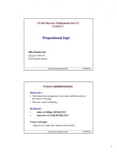
Fig. 3. Left: Church numerals as N-nets



Right: “Fake” Church numerals

To give some more examples, consider the sequent ` a ¯, a ∧ a ¯, a . This is equivalent to the formula (a → a) →(a → a) modulo some applications of associativity and commutativity (here → stands for implication). Hence, the proofs of that sequent can be used to encode the Church numerals. Figure 3 shows on the left the encodings of the numbers 0 to 4 as N-nets. Observe that using B-nets, we can distinguish only the numbers 0, 1, and 2, because all numbers ≥ 2 are collapsed. Note that there are also proofs of that sequent that do not encode a numeral. There are two examples on the right of Figure 3. The top one is obtained by simply mixing together the two proofs 0 and 2. One of the arguments for not having the mix rule in a system is that it causes types (resp. formulas) to be inhabited by more terms (resp. proofs) than the intended ones. However, we would like to stress the (well-known) fact, that this phenomenon is by no means caused by the mix rule, as the bottom “fake” numeral in Figure 3 shows, which comes from the mix-free sequent proof on the right of Figure 2.

4

Proof nets with cuts

¯ where ♦ is called the cut connective, and where the A cut is a formula A ♦ A, function (−) is defined on formulas as follows (with a trivial abuse of notation): ¯ , (A ∨ B) = A¯ ∧ B ¯. ¯ = a , ¯t = f , ¯f = t , (A ∧ B) = A¯ ∨ B a ¯=a ¯, a 9

A sequent with cuts is a sequent where some of the formulas are cuts. But cuts are not allowed to occur inside formulas, i.e., all ♦-nodes are roots. A prenet with cuts is a prenet P B Γ , where Γ may contain cuts. The ♦-nodes have the same geometric behavior as the ∧-nodes. Therefore the correctness criterion has to be adapted only slightly: 4.1 Definition A conjunctive resolution of a prenet P B Γ with cuts is a sub-prenet P |Γ 0 B Γ 0 where Γ 0 has been obtained by deleting one child subformula for every ∧-node and every ♦-node of Γ . 4.2 Definition A W -prenet P B Γ with cuts is said to be correct if for every one of its conjunctive resolutions P |Γ 0 B Γ 0 the W -linking P |Γ 0 is not the zero function. A W -net with cuts is a correct W -prenet with cuts. An example of a correct net with cuts (taken from [12]): ................................................ ........... . ..... .......... .......... ... ¯b ¯b b2 a a ¯ 2 2 ∧



∧



♦



.................................................. ........ .. ... .......... .......... ..... ¯b b2 a a ¯2 b ∧



∧

(6)



In the translation from sequent proofs containing the cut rule into prenets with cuts, the cut is treated as follows: cut

Γ, A

¯ ∆ A,

Γ, ∆

;

cut

¯ ∆ Q B A, ¯ ∆ P ⊕ Q B Γ, A ♦ A, P B Γ, A

.

Here the cut connective is used to keep track of the cuts in the sequent proof. To the best of our knowledge the use of a special connective for cut comes from [23] (see also [16]). In order to simplify the presentation and maintain the similarity between cut and conjunction, our sequent calculus allows contraction to be applied to cut formulas. This slightly unconventional rule is used only for obtaining a generic proof of sequentialization; in no way does it affect the other results (statements or proofs) in the rest of this paper. The generalization of soundness and completeness is now immediate: 4.3 Theorem (Soundness) For any W and any i ∈ {0, 1, 2}, a sequentializable W -prenet in CLi with cuts is correct. 4.4 Theorem (Sequentialization) For any i ∈ {0, 1, 2}, a B-net in CLi with cuts is sequentializable in CLi + cut.

5

Cut elimination

Cut elimination in CL-nets has much in common with multiplicative proof nets. The cut-reduction step on a compound formula is exactly the same: ¯ Γ → P B A ♦ A, ¯ B ♦ B, ¯ Γ P B (A ∧ B) ♦ (A¯ ∨ B), and so it does not affect the linking itself (although we have to show it preserves correctness). The really interesting things happen in the atomic case, which this 10

time splits in two: atomic formulas or constants. Here cut elimination means “counting paths through the cuts”. Let us illustrate the idea by an example: .................... ............. ........................ ...... ........ ...................... a ¯ a ¯ a ¯ a2 ♦



........................... ... .......... ..... a ¯ a a

reduces to

................................................ ......................................................................... .............. .................................................................................... . . a ¯ a ¯ a ¯ a a

More generally, if some weights are different from 1, we multiply them: p

q

r

m

n

_ _ _ _ _ {a ¯1 a4 , a ¯2 a4 , a ¯3 a4 , a ¯5 a6 , a ¯5 a7 } B a ¯1 , a ¯2 , a ¯ 3 , a4 ♦ a ¯ 5 , a6 , a7 pn

pm

qn

qm

rm

rn

_ _ _ _ _ _ ¯3 a6 , a ¯3 a7 } B a ¯1 , a ¯2 , a ¯ 3 , a6 , a7 . ¯2 a7 , a ¯2 a6 , a ¯1 a7 , a → {a ¯1 a6 , a In the case of constants we have for example (here two cuts are reduced): p

q

r

_ _ _ { t1 t1 , f 2 t3 , f 4 t5 } B t1 ♦ f 2 , t3 ♦ f 4 , t 5 To understand certain subtleties let us consider p q r s _ _ _ _ ¯1 a2 , a2 a ¯3 , a ¯3 a4 } B a ¯ 1 , a2 ♦ a {a ¯1 a4 , a ¯ 3 , a4

pqr

_ { t5 t5 } B t5

→

.

z

→

_ ¯ 1 , a4 {a ¯1 a4 } B a

.

What is the value of z? We certainly cannot just take q · s, we also have to add p. But the question is what happens to r, i.e., is the result z = p + qs or z = p + q · (1 + r) · s = p + qs + qrs or even z = p + q · (1 + r + r2 + r3 + · · · ) · s? All choices lead to a sensible theory of cut elimination, but here we only treat the first, simplest case: we drop r. In [18], this property is called loop-killing. Let us now introduce some notation. Given P B Γ and x, y, u1 , u2 , . . . , un ∈ _ L (Γ ), with n even, we write P ( x_u1 · u_ 2 u3 · . . . · un y ) as an abbreviation for P (x, u1 ) · P (u2 , u3 ) · . . . · P (un , y). In addition we define _ u1 · u_ P ( x_ 2 u3 · . . . · un y ) ( _ _ _ P ( x u1 · u2 u3 · . . . · un_y ) + P ( x_un · . . . · u_ if y 6= x 3 u2 · u1 y ) = _ _ _ _ _ _ P ( x u · u u · . . . · u u ) + P ( x u · . . . · u u · u u ) if y = x 1

2

3

n

n

n

3

2

1

1

Notice that in both cases one of the summands is always zero, and that the second case applies only when x is a t and a t1 -axiom is involved. We now can define cut reduction formally for a single atomic cut: y) u · v_ P B u ♦ v, Γ → Q B Γ , where Q(x, y) = P (x, y) + P ( x_ for all x, y ∈ L (Γ ), and where u is labelled by an arbitrary atom or constant, and v by its dual. But we can go further and do simultaneous reduction on a set of atomic cuts: P B u1 ♦ v1 , u2 ♦ v2 , . . . , un ♦ vn , Γ → Q B Γ

,

(7)

where each ui labelled by an arbitrary atom or constant, and vi by its dual. For defining Q, we need the following notion: A cut-path between x and y in a net P B ∆ with x, y ∈ L (∆) is an expression _ _ of the form x_w1 · z_ 1 w2 · z2 w3 · . . . · zk y where wi ♦ zi are all distinct atomic _ _ w1 · z_ cuts in ∆, and such that P ( x_ 1 w2 · z2 w3 · . . . · zk y ) 6= 0. For a set S of 11

atomic cuts in ∆, the cut-path is covered by S if all the wi ♦ zi are in S, and it touches S if at least one of the wi ♦ zi is in S. The Q in (7) is now given by X _ w1 · z_ Q(x, y) = P (x, y) + P ( x_ 1 w2 · . . . · zk y ) , _ _ _ { x w · z w ·...· z y } 1

1

2

k

where the sum ranges over all cut-paths covered by {u1 ♦v1 , u2 ♦v2 , . . . , un ♦vn }. 5.1 Lemma Let P B ∆ be a W -prenet in CLi , and let P B ∆ → P 0 B ∆0 . Then P 0 B ∆0 is also in CLi . Furthermore, if P B ∆ is correct, then P 0 B ∆0 is also correct. The proof is an ordinary case analysis, and it is the only place where Axiom (2) is used. The next observation is that there is no infinite sequence P B Γ → P 0 B Γ 0 → P 00 B Γ 00 → · · · , because in each reduction step the size of the sequent (i.e., the number of ∧, ∨ and ♦-nodes) is reduced. Therefore: 5.2 Lemma The cut reduction relation → is terminating. Let us now attack the issue of confluence. Obviously we only have to consider atomic cuts; let us begin when two singleton cuts: P B ai ♦ a ¯ j , ah ♦ a ¯k , Γ are reduced. If the first cut is reduced, we get P 0 B ah ♦ a ¯k , Γ , where P 0 (x, y) = ai · a y ). Then reducing the second cut gives us Q1 B Γ , where P (x, y) + P ( x_ ¯j_ 0 ah · a y ). An easy computation shows that Q1 (x, y) = P (x, y) + P 0 ( x_ ¯k_ _ y )+ ai · a y ) + P ( x_ ah · a y ) + P ( x_ ai · a ¯j ak · a ¯h_ ¯h_ ¯j_ Q1 (x, y) = P (x, y) + P ( x_ (8) _ _ _ ai · a y ) . ah · a y ) + P ( x_ ¯j ah · a ¯k ai · a ¯k ai · a ¯j_ P ( x_ ¯j_

Reducing the two cuts in the other order yields Q2 B Γ , where _ y )+ ai · a y ) + P ( x_ ah · a y ) + P ( x_ ai · a ¯j ak · a ¯h_ ¯k_ ¯j_ Q2 (x, y) = P (x, y) + P ( x_ (9) _ _ _ ah · a y ) . ah · a y ) + P ( x_ ¯k ai · a ¯k ai · a ¯j ah · a ¯k_ P ( x_ ¯j_

We see that the last summand is different in the two results. But if we reduce both cuts simultaneously, we get Q B Γ , where y )+ y ) + P ( x_ ah · a ai · a ¯k_ Q(x, y) = P (x, y) + P ( x_ ¯j_ _ _ y ) y ) + P ( x_ ah · a ai · a ¯k ai · a ¯j_ P ( x_ ¯j ak · a ¯h_

(10) .

Now the troublesome summand is absent. There are also good news: In the case of B-nets we have that Q = Q1 = Q2 . The reason is that if in either Q1 or Q2 the last summand is 1, then at least one of the other summands is also 1. This ensures that the whole sum is 1, because of idempotency of addition. Therefore: 5.3 Lemma On B-prenets the cut reduction relation → is locally confluent. Lemmas 5.1–5.3 together give us immediately: 5.4 Theorem On B-nets cut elimination via → is strongly normalizing. The normal forms are cut free B-nets. Note that we do not have this result for general W . Let us compare our cut elimination with other (syntactic) cut elimination procedures for classical propositional logic. In the case of B-nets, the situation 12

.............................. ................................................................................................................................................... . ................. ............... .............. ............ ....... . . . . . . . . . . . . . . . . . ... .... .. .... ..... ..... .... .... .......... ............. .......... ...... ... .... .......... ¯ ¯ ¯ ¯b a a ¯/ b ¯/ b b / a a ¯/ b b / a a /



∧ OOO











∧ OOOoo ∧

oo ∧

∧

OOO oooOOO ooo Ho Ho

!

∧

∧

................................................................................ .................................................... .............. ....................................... ................................................................. ......... . . . . . ... .... ... .. ..... .. ... ..... .......... .......... ..... .... .......... ..... ............. ¯b b a a ¯b a a ¯ b b a a ¯ ¯ / b ! / / / / /



∧



∧



 ∧ o o OOO oooOOO ooo Ho Ho

∧ OOO



............................................ ........................... ......................................................................................................................... . . . . . ..... .. .. ...... ............. .... .... ... .............. .......... ....... ... ... ..... ................ ¯ ¯b 2 a a¯ 2 b b 2 a a¯ 2 b



∧ OOOoo ∧



∧



∧



∧



............................................. .......................... . ............................................................................................................................. . . . . . .......... ........ ... . . .............. . . . . ................ .......... . .. .... .... . .... .. .. .. .. . ¯ ¯b 2 a a¯ 2 b b 2 a a¯ 2 b ∧



∧



∧



∧



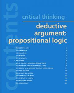
Fig. 4. The two different results of applying sequent calculus cut elimination to the proof (6). Left: Written as Girard/Robinson proof-net. Right: Written as N-proof-net.

is quite similar to the sequent calculus: the main differences is that we do not lose any information in the weak-weak case, although we lose some information of a numeric nature in the cont-cont case. In the case of N-nets, the situation is very different. Let us use (6) for an example. The sequent calculus cut elimination needs to duplicate either the righthand side proof or the left-hand side proof. The two possible outcomes, together with their presentation as N-nets, are shown in Figure 4, where the H stand for contractions3 . However, in our setting, the result of eliminating the cut in (6) is always (3), whether we are in B-nets or in N-nets. Although for N-nets the cut elimination operation does not have a close relationship to the sequent calculus, there is a good correspondence with cut elimination in the calculus of structures, when done via splitting [14]. We do not have confluence in general, but at least, given a sequent with cuts, there is a “most canonical” way of obtaining a cut-free proof net: do simultaneous elimination of all the cuts at once.

6

A bit of abstract nonsense

For i ∈ {0, 2}, let CLBi denote the category whose objects are the CLi -formulas and whose arrows are the cut-free B-nets (in CLi ) that have two (ordered) conclusions: ¯ B is a map from A to B. The composition of two maps P B A, ¯ B P B A, ¯ ¯ ¯ and Q B B, C is given by eliminating the cut on P ⊕ Q B A, B ♦ B, C. The associativity of that operation is a direct consequence of Theorem 5.4. In CLB0 and CLB2 there is an obvious identity map for every object. CLB1 is not a category because it does not have identities: this is easy to check for t. 3

This idea of using explicit contraction nodes was sketched in [12] and is carried out in detail in [24].

13

Given a general W , it is not certain that we can adapt the construction [10] to get a category, where the objects would be the CLi -formulas but where the arrows would be the two-conclusion W -nets in which atomic cuts may be present. One of the main points of that construction is that it allows the definition of an enrichment in posets—more correctly, sup-semilattices—where bigger nets for that order are nets that have more cuts. But then in our case there is always a naturally defined commutative monoid “enrichment”, given by pointwise sum of nets, which is the corresponding structure. In what follows we will sketch the axiomatic structure that the CLBi possess, allowing comparison with the categorical formalisms that have been recently proposed. It is not hard to show that we do get a *-autonomous category, with the expected interpretation (tensor is ∧, the involution is (−), etc.); but not one that has units in general (new developments on the concept of unitless autonomous category can be found in [18]). This makes our semantics rather similar to [10, 11] (which, as we have said, is based on a rather different notion of proof net). But it does not seem that the categories proposed in [9] can be *-autonomous without being posets. In the case of CLB2 , the ∧ does have a unit t of some sort, but the standard unit laws are not exactly true: there is a natural map λA : t ∧ A → A, (and thus, because of the symmetry, a ρA : A ∧ t → A) and they obey the “standard diagram” [21, p. 159], but they are not isomorphisms. Instead λ only has a right inverse λ∗A : A → t ∧ A, with λA ◦ λ∗A = 1A . It is not hard to generalize the notion of symmetric monoidal category to accommodate that situation; this includes a suitable coherence theorem. But naturally our categories have more: there is diagonal map ∆A : A → A ∧ A, and the counit map !A : A → t which exists in CLB2 and which can be replaced for CLB0 by the usual projection map A ∧ X → X, which is natural in X. Thus we can say that every object is equipped with a ∧-comonoid structure (and by duality a ∨-monoid structure), when these notions are adapted to fit the absence of real units to ∧, ∨. All the recent proposals for “Boolean” categories have this structure; it is by now clear that the reason that we do not have collapse to a poset is that the families (∆A )A and (!A )A are not natural. Some additional important equations on the interaction between the *-autonomous and the monoid-comonoid structure are in [18]; a general “covariant” treatment of these issues is in [9]. Our logic gives us a natural map mixA,B : A ∧ B → A ∨ B. Thus given any pair of parallel maps f, g : A → B we can construct (see also [9]) f + g = ∇B ◦ (f ∨ g) ◦ mixA,A ◦ ∆A .4 It is then easy to check that this operation is commutative and associative. (But in general it does not give us an enrichment of CLBi over the category of commutative semigroups.) Thus the sum of linkings (see Section 2) can be recovered through the categorical axioms. Since W = B here the additional axiom f + f = f of idempotency holds; thus in this case every hom-set does have a sup-semilattice structure. 4

It has recently been shown that the semilattice enrichment mentioned above can also be obtained that way [11].

14

References 1. Peter B. Andrews. Refutations by matings. IEEE Transactions on Computers, C-25:801–807, 1976. 2. Kai Br¨ unnler and Alwen Fernanto Tiu. A local system for classical logic. In LPAR 2001, volume 2250 of L, pages 347–361. Springer-Verlag, 2001. 3. Samuel R. Buss. The undecidability of k-provability. Annals of Pure and Applied Logic, 53:72–102, 1991. 4. Alessandra Carbone. Interpolants, cut elimination and flow graphs for the propositional calculus. Annals of Pure and Applied Logic, 83:249–299, 1997. 5. Stephen A. Cook and Robert A. Reckhow. The relative efficiency of propositional proof systems. The Journal of Symbolic Logic, 44(1):36–50, 1979. 6. Thierry Coquand. A semantics of evidence for classical arithmetic. The Journal of Symbolic Logic, 60(1):325–337, 1995. 7. V. Danos, J.-B. Joinet, and H. Schellinx. A new deconstructive logic: Linear logic. The Journal of Symbolic Logic, 62(3):755–807, 1997. 8. Kosta Doˇsen. Identity of proofs based on normalization and generality. The Bulletin of Symbolic Logic, 9:477–503, 2003. 9. Kosta Doˇsen and Zoltan Petri´c. Proof-Theoretical Coherence. KCL Publications, London, 2004. 10. Carsten F¨ uhrmann and David Pym. On the geometry of interaction for classical logic (extended abstract). In LICS 2004, pages 211–220, 2004. 11. Carsten F¨ uhrmann and David Pym. Order-enriched categorical models of the classical sequent calculus. 2004. 12. Jean-Yves Girard. A new constructive logic: Classical logic. Mathematical Structures in Computer Science, 1:255–296, 1991. 13. Jean-Yves Girard, Yves Lafont, and Paul Taylor. Proofs and Types. Cambridge Tracts in Theoretical Computer Science. Cambridge University Press, 1989. 14. Alessio Guglielmi. A system of interaction and structure, 2002. To appear in ACM Transactions on Computational Logic. On the web at: http://www.ki.inf.tudresden.de/˜guglielm/Research/Gug/Gug.pdf. 15. Alessio Guglielmi and Lutz Straßburger. Non-commutativity and MELL in the calculus of structures. In Laurent Fribourg, editor, Computer Science Logic, CSL 2001, volume 2142 of LNCS, pages 54–68. Springer-Verlag, 2001. 16. Dominic Hughes and Rob van Glabbeek. Proof nets for unit-free multiplicativeadditive linear logic. In LICS 2003, pages 1–10. 2003. 17. J. Martin E. Hyland. Abstract interpretation of proofs: Classical propositional calculus. In CSL 2004, volume 3210 of LNCS, pages 6–21. Springer-Verlag, 2004. 18. Fran¸cois Lamarche and Lutz Straßburger. Constructing free Boolean categories, 2005. Submitted. 19. Olivier Laurent. Etude de la Polarisation en Logique. PhD thesis, Univ. AixMarseille II, 2002. 20. Olivier Laurent. Polarized proof-nets and λµ-calculus. Theoretical Computer Science, 290(1):161–188, 2003. 21. Saunders Mac Lane. Categories for the Working Mathematician. Number 5 in Graduate Texts in Mathematics. Springer-Verlag, 1971. 22. Michel Parigot. λµ-calculus: An algorithmic interpretation of classical natural deduction. In LPAR 1992, volume 624 of LNAI, pages 190–201, 1992. 23. Christian Retor´e. Pomset logic: A non-commutative extension of classical linear logic. In TLCA 1997, volume 1210 of LNCS, pages 300–318, 1997. 24. Edmund P. Robinson. Proof nets for classical logic. Journal of Logic and Computation, 13:777–797, 2003.

15