one will be called S1, the second S2 and the third S3. A similar ...... Figure 19: Absorbance spectra of a 5% weight per volume solution of holmium oxide in.
Nanometrology using Time-Resolved Fluorescence Techniques Philip Yip A thesis presented in partial fulfilment of the requirements for the degree of Doctor of Philosophy
Department of Physics, Photophysics Research Group University of Strathclyde HORIBA Scientific IBH National Physical Laboratory Biotechnology Group HORIBA Scientific ISA March 2016
ii
This thesis is the result of the author’s original research. It has been composed by the author and has not been previously submitted for examination which has lead to the award of a degree. The copyright of this thesis belongs to the author under the terms of the United Kingdom Copyright Act as qualified by the University of Strathclyde regulation 3.50. Due acknowledgement must always be made for the use of the material contained in, or derived, from this thesis.
Signed:
Date:
iii
Acknowledgements I would like to thank the Photophysics Research group, University of Strathclyde especially my supervisors David Birch and Yu Chen for all the advice and assistance they gave me throughout my PhD and the technicians John Revie and Andre Hughes for all the wonders they made in the mechanical workshop. I would like to thank all the support I got from everyone at HORIBA Scientific IBH and ISA especially my industrial supervisors Graham Hungerford, David McLoskey, Jim Mattheis and Ishai Nir for answering my never-ending series of questions and in particular, for all the fluorescence instrumentation expertise I picked up from working with them. I would also like to thank everyone from NPL in particular my industrial supervisor Alex Knight for the microscopy expertise I picked up working with him. I would like to thank Josh Barham from Department of Pure and Applied Chemistry, University of Strathclyde and API Chemistry, Platform Technology and Science, GlaxoSmithKline for Chemistry expertise. I would like to thank SUPA for the SUPA Inspire studentship, SUPA short-term visit and SUPA secondment to IBH which allowed me to carry out my PhD in such close collaboration with industry. I would also like to thank my family for morale support.
iv
Abstract This thesis looks at fluorescence techniques and their use for nanometrology applications. It has been primarily industrially linked with scientific instrument vendors Horiba Scientific IBH and Horiba Scientific ISA and examines the state of the art instrumentation taking the reader from grounds up from simple steady-state and time-resolved fluorescence spectroscopy techniques that are routinely used and newer more advanced techniques made possible but rapid developments in technology. Secondary industrial links are to NPL allowing the examination of the state of the art instrument in fluorescence microscopy an extension of fluorescence spectroscopy and this thesis likewise builds from simple to advanced microscopy techniques. In the case of nanometrology well-established techniques in particular timeresolved fluorescence anisotropy, which overcomes the diffraction barrier by use of low concentrations and infers the average particle size of a homogeneous distribution by use of polarized light and Brownian motion are discussed. These applications are examined in conjunction to high concentration microscopy techniques such as direct Stochastic Optical Reconstruction Microscopy (dSTORM) High concentration heterogeneous techniques are better suited to most biological applications which involve the measurement of highly packed nanostructures. dSTORM requires use of specific chemical conditions and high laser power to enable stochastic blinking. A video of these stochastic blinks by use of a fast capture imaging CCD allows one to temporally resolve each single-molecule blinks and construct a single super-resolution image. The implication of these chemical conditions, high laser power and limitations even in today’s state of the art CCDs need to be properly understood and any development in either but preferably all three will make this advanced microscopy technique more feasible. This work looks at the properties of some new probes for nanometrology however, the strict criteria required for successful dSTORM applications in particular leaves this work an open investigation.
v
List of Abbreviations xxxx/yyy grating – grating blazed to optimise output at yyy nm and xxxx lines/mm. xxxx/yyy double grating – double grating blazed to optimise output at yyy nm and xxxx lines/mm. A – Signal from Auxiliary port, usually from a photodiode. Ac – Corrected signal from Auxiliary port accounting for excitation wavelength correction factors and dark counts. APS – 3-aminopropyl trimethoxysilane. AFM – Atomic Force Microscopy. Auxx – xx number of atoms in a gold nanocluster. Auxx@BSA – xx number of atoms in a gold nanocluster encapsulated by Bovine Serum Albumin. Auxx@HSA – xx number of atoms in a gold nanocluster encapsulated by Human Serum Albumin. Auxx@GSH – xx number of atoms in a gold nanocluster encapsulated by Glutathione. BPxxx/yy – Bandpass filter at xxx nm. Spectral Full width half maximum of yy nm. BDR – Best Dynamic Range. Number of electrons per count setting which offers the best dynamic range for a Charged Coupled Device. BSA – Bovine Serum Albumin CCD – Charge Coupled Device. CPS – Counts per second. Cuxx – xx number of atoms in a copper nanocluster. Cuxx@BSA – xx number of atoms in a copper nanocluster encapsulated by Bovine Serum Albumin. DAEEM – Decay Associated Excitation Emission Matrix (not weighted by the decay time). DAEEMW – Decay Associated Excitation Emission Matrix weighted by the decay time. DAS – Decay Associated Spectra (not weighted by decay time). Emission unless otherwise stated. DASW – Decay Associated Spectra weighted by decay time. Emission unless otherwise stated. DDxxxD – DeltaDiode pulsed diode source at xxx nm peak wavelength. Maximum repetition rate = 20 MHz. DDxxxD – DeltaDiode pulsed laser source at xxx nm peak wavelength. Maximum repetition rate = 100 MHz. dSTORM – direct Stochastic Optical Reconstruction Microscopy. EEM – Excitation Emission Matrix. FCS – Fluorescence Correlation Spectroscopy. FCCS – Fluorescence Cross-Correlation Spectroscopy. FF – Front Face Geometry. FITC – Fluorescein Isothiocyanate. FITC- APS – Fluorescein Isothiocyanate coupled to 3-aminopropyl trimethoxysilane. FLIM – Fluorescence Lifetime Imaging Microscopy. FLCS – Fluorescence Lifetime Correlation Spectroscopy. FWHM – Full Width at Half Maximum. GSH – glutathione/ H – Polarizer orientation is horizontal 90°1. 1
When two polarizers are used. The first letter represents the orientation of the excitation polarizer and the second one represents the orientation of the emission polarizer.
vi
HL – High Light. Number of electrons per count setting which accommodates the best setting for high light intensity when using a Charged Coupled Device. HS – High Sensitivity. Number of electrons per count setting which accommodates the best setting for high sensitivity when using a Charged Coupled Device. HSA – Human Serum Albumin LPxxx – Long Pass filter at xxx nm. M – Polarizer orientation is at the Magic Angle 54.7°1. MCorrect – Emission Wavelength correction factor for detector on S2. MCP – Multi-channel plate photomultiplier tube detector. MCS – Multi-channel scaling. N – No Polarizer present NLxxxD – NanoLED pulsed diode at xxx nm peak wavelength. Maximum repetition rate = 1 MHz. NLxxxL – NanoLED pulsed laser at xxx nm peak wavelength. Maximum repetition rate = 1 MHz. NDx.x – Neutral Density filter x.x represents the grade. NTA – Nanoparticle Tracking Analysis. PARAFAC – Parallel Factor Analysis. PMT – Photomultiplier Tube. POPOP – 1,4-bis(5-phenyloxazol-2-yl) benzene PTxx – xx number of atoms in a platinum nanocluster. PTxx@BSA – xx number of atoms in a Platinum nanocluster encapsulated by Bovine Serum Albumin. R – Reference signal from excitation arm photodiode. RA -Right Angle geometry. Rc – Corrected reference accounting for excitation wavelength correction factors and dark counts. S – Signal from emission arm. This is commonly the right arm when facing the fluorimeter3. Sc – Corrected signal accounting for emission wavelength correction factors and dark counts. SIM – Structured Illumination Microscopy. SLxxxD – SpectraLED diode at xxx nm peak wavelength. SNR – Signal to Noise Ratio. SNRFSD – Signal to Noise Ratio First Standard Deviation. SNRRMS – Signal to Noise Ratio Root Mean Square. SPxxx – Short Pass filter at xxx nm. SS – Steady-State. SSFA – Steady-State Fluorescence Anisotropy. STED – Stimulated Emission Depletion Microscopy. T – Signal from emission arm. This is commonly the right arm when facing the fluorimeter3. TAC – Time to Amplitude Convertor. TCSPC – Time Correlated Single Photon Counting. TCorrect – Emission Wavelength correction factor for detector on T2. TDM – Time Domain Discriminator. TR – Time Resolved 2
If multiple detectors are mounted on S and T or multiple gratings used the names MCorrect and TCorrect will usually state, the grating, name of the detector and the emission arm. 3 The first detector on the S emission arm is S1. In cases where there are multiple detectors mounted the first one will be called S1, the second S2 and the third S3. A similar nomenclature is used for the T emission arm.
vii
TREEM – Time-Resolved Excitation Emission Matrix. TRFA – Time-Resolved Fluorescence Anisotropy. TRES – Time Resolved Emission Spectrum. TRIZMA – 2-Amino-2-(hydroxymethyl)-1,3-propanediol. Try-xxx – Trytophan amino acid at amino acid position xxx. V – Polarizer orientation is vertical 0°1. XCorrect – Excitation Wavelength correction factor.
List of Publications Stewart H L, Yip P, Rosenberg M, Sørensen T J, Laursen B W, Knight A E and Birch D J S 2016 Nanoparticle metrology of silica colloids and super-resolution studies using the ADOTA fluorophore Meas. Sci. Technol. 27 045007 Birch D J S and Yip P 2014 Nanometrology Fluorescence Spectroscopy and Microscopy: Methods and Protocols Methods in Molecular Biology vol 1076, ed Y Engelborghs and A J W G Visser (Totowa, NJ: Humana Press) pp 279–302 Gracie K, Smith W E, Yip P, Sutter J U, Birch D J S, Graham D and Faulds K 2014 Interaction of fluorescent dyes with DNA an spermine using fluorescence spectroscopy. Analyst 139 3735–43 Wu Y, Stefl M, Olzyńska A, Hof M, Yahioglu G, Yip P, Casey D R, Ces O, Humpolíčková J and Kuimova M K 2013 Molecular rheometry: direct determination of viscosity in Lo and Ld lipid phases via fluorescence lifetime imaging. Phys. Chem. Chem. Phys. 15 14986– 93 Yip P, Karolin J and Birch D J S 2012 Fluorescence anisotropy metrology of electrostatically and covalently labelled silica nanoparticles Meas. Sci. Technol. 23 084003
Conference Proceedings Yip P, Hungerford G, Knight A, Chen Y and Birch D J S 2015 The Spectroscopy of Au25@BSA Nanoclusters and their Application for dSTORM) 2015 FluoroFest Presentation http://www.fluorofest.org/ Yip P, Knight A and Birch D J S 2015 Direct Stochastic Optical Reconstruction Microscopy 2015 SUPA Annual Meeting 6 Minute Video
viii
Yip P, Hungerford G, Knight A, Chen Y and Birch D J S 2014 The Spectroscopy of Au25@BSA Nanoclusters and their Potential use as Probes for direct Stochastic Optical Reconstruction
Microscopy
(dSTORM)
2014
FluoroFest
Presentation
http://www.fluorofest.org/ Yip P, Hungerford G, Knight A, Chen Y and Birch D J S 2014 The Potential Use of Au25@BSA as Probes for direct Stochastic Optical Reconstruction Microscopy (dSTORM) 2014 SULSA Research Symposium Optical Imaging of Cells: From Single Molecules to Organelles Poster Yip P, Hungerford G, Knight A, Chen Y and Birch D J S 2014 The Investigation of the Fluorescence Profile of BSA Encapsulated Au25 Nanoclusters as New Probes for Super Resolution Microscopy Instruments & Methods for Biology and Medicine 2014 Presentation http://imbm.fbmi.cvut.cz/ Yip P, MacMilliam A, Knight A, Sutter J, Chen Y and Birch D J S 2013 Fluorescence Imaging of Single Gold Nanoclusters Methods and Application in Fluorescence 2013 Poster http://www.maf13.org/ Yip P, Hungerford G, Knight A, McCalf D, Chen Y and Birch D J S 2013 A Nano-Toolbox for Biomolecular Fluorescence Imaging 2013 SUPA Physics and the Life Sciences Poster http://www.supa.ac.uk/Research/PaLS/2013-PaLS-meeting Yip P and Birch D J S 2011 Nanoparticle Metrology Using Covalently Labelled Fluorescence Probes 2012 PiMoP Prague Workshop on Photoinduced Molecular Processes Presentation http://pimop2012.fjfi.cvut.cz/ Yip P, Hungerford G, Knight A, McCalf D, Chen Y and Birch D J S 2012 A Nano-Toolbox for Biomolecular Fluorescence Imaging 2012 SUPA Inspire Annual Meeting Poster http://www.supa.ac.uk/inspire-annual-meeting/2012-inspire-annual-meeting Yip P, Karolin J and Birch D J S 2011 Fluorescence Depolarisation of Covalently Labelled Silica Nanoparticles 2011 Nano Meets Spectroscopy Poster Yip P, Karolin J and Birch D J S 2011 A Nano-Toolbox for Biomolecular Fluorescence Imaging 2011 SUPA Inspire Annual Meeting Poster http://www.supa.ac.uk/inspire-annualmeeting/2011-inspire-annual-meeting
ix
Contents Acknowledgements ............................................................................................................. iv Abstract ................................................................................................................................ v List of Abbreviations .......................................................................................................... vi List of Publications .......................................................................................................... viii Conference Proceedings................................................................................................... viii 1. Introduction ...................................................................................................................... 1 1.1
Fluorescence Spectroscopy ................................................................................... 3
2. Experimental Details ...................................................................................................... 21 2.1 Absorbance – Spectrophotometer ............................................................................ 21 2.1.1 Spectrophotometer Calibration ......................................................................... 24 2.1.2 Transmission of Optical Components and Filters ............................................. 28 2.1.3 Limitations ........................................................................................................ 30 2.2 Emission – Spectrofluorimeter ................................................................................ 32 2.2.1 Monochromator Calibration and Signal to Noise ............................................. 36 2.2.2 Corrected Excitation and Emission Spectra ...................................................... 40 2.2.3 Monochromator Bandpass ................................................................................ 53 2.2.4 Detector Type.................................................................................................... 59 2.2.5 The Excitation-Emission Matrix (EEM) ........................................................... 68 2.2.6 Highly Concentrated Samples – The Front Face Measurement ....................... 82 2.2.7 Steady State Fluorescence Anisotropy.............................................................. 84 2.3 Time Resolved Emission – Spectrofluorometer ...................................................... 91 2.3.1 Measuring a Long Lived Phosphorescent Fluorescence Decay with Simple Electronics.................................................................................................................. 96 2.3.2 Multi-Channel Scaling (MCS) ........................................................................ 101 2.3.3 Time Correlated Single Photon Counting Principle ....................................... 105 2.3.4 Instrumental Response .................................................................................... 108
x
2.3.5 Delay lines, Repetition Rate and TAC Range ................................................ 115 2.3.6 Time Calibration ............................................................................................. 119 2.3.7 Data Fitting - Fluorescence Decay Curves ..................................................... 121 2.3.8 Fluorescence Decay Measurements – The Magic Angle ................................ 126 2.3.9 Time-Resolved Fluorescence Anisotropy Decay Measurements ................... 128 2.3.10 Time-Resolved Emission Spectra (TRES) and Decay Associated Spectra (DAS) ....................................................................................................................... 145 2.3.12 Time Resolved Excitation Emission Matrix (TREEM) and Decay Associated Excitation Emission Matrix (DAEEM) ................................................................... 159 2.3.13 Kinetic TCSPC.............................................................................................. 163 2.4 Confocal Microscopy ............................................................................................. 168 2.4.1 Confocal Microscopy Techniques and the Diffraction Limit ......................... 168 2.4.2 Confocal Nanoscopy Techniques ................................................................... 173 2.4.3 Location Nanoscopy ....................................................................................... 177 3.
Nanometrology using TRFA.................................................................................... 188 3.1 Protein .................................................................................................................... 188 3.2 Silica Nanoparticles ............................................................................................... 191
4. Spectroscopy of AzaDiOxaTriAngulenium (ADOTA) Fluorophores and their use for Nanometrology ................................................................................................................ 197 4.1 ADOTA as an Anisotropy Probe? ......................................................................... 198 4.2 ADOTA as a dSTORM Probe?.............................................................................. 211 5. Spectroscopy of Gold Nanoclusters and their use for Nanometrology........................ 220 5.1 Au25@BSA Protein Synthesised Gold Nanoclusters ............................................. 221 5.2 Au25@BSA Protein Synthesised Nanoclusters as a dSTORM Probe? .................. 250 5.3 Au25@GSH Nanoclusters as a dSTORM Probe? .................................................. 255 6. Conclusions .................................................................................................................. 259 7. References .................................................................................................................... 262
xi
1. Introduction The work in this thesis looks at some of the latest developments in fluorescence techniques and fluorescence instrumentation. The application areas of fluorescence spectroscopy are incredibly diverse. As many biological components exhibit fluorescence [1] and organic components [2] have a unique excitation and emission profile the fluorescence excitationemission matrixes may be used to detect any impurities as well as identify the impurity and concentration level via its excitation-emission profile [3]. The fluorescence profile from these biological components also plays an important in food science and as food ages the fluorescence profile which is greatly influenced by its chemical environment will change. Hence if the fluorescence profile of food is characterised for the foods lifecycle then future fluorescence measurements will be able to infer the quality of the food [4–6]. Fluorescence plays a key role for the encryption of documents; every passport or currency note has an embedded fluorescence/phosphorescence pattern which under normal light is not observed but under UV illumination can clearly be seen. Fraudulent documents can easily be identified as it is hard to replicate this pattern without the specialised printing technology and knowhow. More and more sophisticated fluorescence encryption and printing techniques are in demand [7,8]. Fluorescence techniques have potential applications in recycling as the high specificity of fluorescence techniques have the capability to identify different types of plastic flakes which are otherwise hard to distinguish from one another [9,10]. Fluorescence plays a key role in healthcare [11]. With carefully tailored systems, the sensitivity of fluorescence measurements can be taken advantage of and be utilised for specific analyte sensing [12,13]. A great deal of effort has been put into developing sugar specific sugar sensing in particular glucose [14–20]. Fluorescence spectroscopy of blood may be used as a diagnostic to detect disease [21] and the fluorescence profile of cells may be used for cell-sorting [22]. It is also possible to use fluorescence techniques for gas sensing for instance CO2 [23] and O2 [24]. Ion recognition and pH measurements are also possible with fluorescence [25–27] as well as viscosity measurements. By ingenuity of fluorescence measurement parameters including fluorophore, excitation wavelength, emission wavelength, polarization and time-scale of measurement [28] one can tune fluorescence techniques to measure and even visualise structures at nm resolution. Fluorescence spectroscopy and its extension fluorescence microscopy are already very well established techniques and widely used every day particular due to the high sensitivity of 1
fluorophores to their local environment. The most significant research area is that of the life sciences where basic fluorescence measurements are routinely used. Clearly all the application areas mentioned above can be incorporated into measurements of biological organisms. Analyte sensing in complex small µm, heterogeneous biological systems such as the cell requires a sensitive enough technique such as fluorescence [29]. Cellular viscosity measurements for example are made possible with a fluorescence molecular rotor which has a fluorescence lifetime dependant on the viscosity of the probes local environment [30]. A globally recognised application is the well-established area of DNA sequencing [31–36], in particular the Human Genome Project [37–39] which had led to a new era of medical breakthroughs. This project would not have been possible without the aid of fluorescence techniques and the associated rapid development of fluorescence instrumentation [40], fluorescent dyes with appropriate linkers [41] and techniques [42]. Although a vast deal of information has been collected within the life sciences, it can be said that there remain more questions than answers. One of the main difficulties is that in order to visualise biological structures one has to measure at a higher resolution i.e. measure at a nanoscale and the ultimate goal for biological imaging is to measure dynamically in nanoscale at x, y and z for a relatively large objects such as a human being. The last decade has seen a rapid development in fluorescence techniques and the beginning of the exciting frontier of super-resolution microscopy. Pioneering work has been carried out on gene regulation[43], actin filament assembly [44], self-organisation of the ecoli chemotaxis network and the investigation of a full embryo while its developing [45,46]. The main goal of nanometrology fluorescence measurements in the life sciences is to understand how biological organisms work and in cases don’t work. This will allow for the development of new diagnostics and therapeutics as well as the development of new materials or nanomaterials. The work in this thesis was done in conjunction to a fluorescence scientific instrument vendor HORIBA Scientific IBH and HORIBA Scientific ISA and a world renowned centre of nanometrology NPL Biotechnology Group and looks into the applications and developments of high end fluorescence techniques. The first chapter of this thesis will discuss the basic principles behind fluorescence and related phenomenon. The second chapter will build up an understanding of basic fluorescence measurements including system checks to more powerful advanced measurements that aren’t yet fully established. There’s still future scope for some of the techniques discussed. The third
2
chapter examines the use of time-resolved fluorescence anisotropy techniques for nanosizing objects down to 4 nm in radii however this technique has the limitation that a relatively simple system is required. The fourth chapter looks at the complicated spectroscopy and characterisation of Au25 nanoclusters which are a unique type of probe possessing a number of desired characteristics and the fifth chapter looks at the use of these probes for super-resolution microscopy. The last chapter is the conclusion.
1.1 Fluorescence Spectroscopy
Figure 1: Time scale of emission processes with respect to chemical and atomic events. The time scales of emissive processes such as Raman, fluorescence and phosphorescence are on a suitable time-scale allowing investigation of these events. 3
This work focuses on luminescence spectroscopy, primarily fluorescence an emissive process on the ~ns time scale and secondary phosphorescence a longer-lived emissive process on the µs [47]. This work focuses primarily on the field of fluorescence and phosphorescence spectroscopy due to the very convenient time scale of these emissive processes comparable to underlying biological and chemical processes see Figure 1 [40,48]. Fluorescence measurements in particular provide the sensitivity and correct timescales for studying and using reactions and kinetics needed across a wide range of disciplines. Fluorescence is a radiative emission process typically on the ≈ns time scale and phosphorescence is a radiative emission process on the ≈µs-ms time scale. Since the speed of light is 3×10⁸ m s–1, in 1 ns (1×10⁻⁹ s), light travels 30 cm.
Figure 2: Schematic of an electron orbiting around a nucleus using a quantised radius which has the form 𝑦 = 𝐴 sin(𝜔𝑡).
Figure 3: Schematic of an electron orbiting around a nucleus at the quantised ground state. A photon of light can interact with the electron transferring energy to the electron taking it to the quantised first excited state.
4
The underlying processes of fluorescence spectroscopy will now be discussed. Spectroscopy is the investigation of the interaction of matter using electromagnetic radiation. Figure 2 illustrates an ideal classical system, an electron orbiting around a nucleus where the energy of each orbit is quantised. This motion has the form of a sine wave. In an atom or molecule, an electromagnetic wave (such as visible light) can induce an oscillating electric or magnetic moment. Figure 3 a photon of light is equal in energy to the difference between the ground eigenstate Ψ𝑖1 and the first excited eigenstate Ψ𝑗 . A resonance interaction results in the transfer of energy to the electron allowing it to access a higher energy orbit. This is known as an electronic transition. The strength or probability of a transition depends on the overlap of the two waves (in this example both waves being sine waves) and also the phase of both waves (in this example both waves are in phase). In 2
⃗⃗ 𝑗𝑖 | where the quantum mechanics the strength of a transition from Ψ𝑖 to Ψ𝑗 is given by |𝑀 transition dipole moment [49]: M ji j i dV
(1) The integration is performed over all space and 𝜇 is the dipole moment operator, for a collection of charges this is the sum of each individual charge qn multiplied by the distance of each individual charge rn:
qn rn
(2)
n
The mass of an electron is a thousandth of the mass of a proton or neutron hence the most probable vibronic transition is one which involves no change in the nuclear co-ordinates. ⃗⃗ 𝑗𝑖 This assumption is known as the Franck-Condon principle [50–53]. As a consequence, 𝑀 can be separated into electronic and vibrational components. M ji je ie dV jv iv dV
(3)
⃗⃗ 𝑗𝑖 separately the probability of an electronic transition Examining the vibrational part of 𝑀 from one vibrational energy to another will be more likely to occur if the vibrational wavefunctions of the two states overlap see Figure 4, these are known as Franck-Condon factors. Now consider a molecule in which only the vibrational mode is dominant, so that it approximates to a harmonic oscillation. The solutions of the simple harmonic oscillator are a fundamental problem in any quantum mechanics textbook. A state involving
5
electronic and vibrational energy is referred to as a vibronic state. Let the energy of the vibronic state be Et. If the electronic energy of the ground state is Ee and the energy of the fundamental vibrational mode in the ground state is Ev then the total energy Et:
1 Et Ee m Ev 2
(4)
where m=0,1,2,… is the vibrational quantum number. An electronic excited state is characterised by certain basic properties; its energy its multiplicity and its symmetry [53]. To reach an electronic state higher than the ground state the fluorophore (fluorescent species) must first absorb light energy. Once energy is absorbed because the nuclear coordinates are unchanged the vibronic energy of the excited state 𝐸𝑡′ :
1 Et' Ee' n Ev' 2
(5)
where n=0,1,2,…, 𝐸𝑒′ is the electronic energy in the excited state and 𝐸𝑣′ is the energy of the fundamental vibrational mode in the excited electronic state.
Figure 4: Illustration of the Franck-Condon principle alongside the assumption that the vibrational mode is dominant approximating to that of a simple harmonic oscillator. The purple curves denote the wavefunctions of each vibronic state. The intensity of lines is partially governed by the overlap of the vibrational wavefunctions denoted as purple lines
6
these are known as Franck Condon states. The blue absorption line 0-2 will give a strong band in the absorbance spectrum and the red emission line 0-2 will give a strong emission band in the emission spectrum because of the good overlap between the Franck Codon states. The absorption and emission lines are shown as straight lines as the assumption of no changes in the nuclear co-ordinates during vibronic transitions has been made.
If the ground state is in thermal equilibrium at absolute temperature T the fraction fm of ground state molecules in a vibrationally excited state m is determined by the Boltzmann factor:
mE f m exp v kT
(6)
where k is Boltzmanns constant 1.38×10⁻²³ J K–1, T is the temperature in K and: 1 1 Ev hc 1 2
(7)
where h=6.34×10⁻³⁴ J s is Planck’s constant, c≈3×10⁸ m s–1 is the speed of light and 1 is the first and 2 is the second emission maxima. In the case of Perylene Figure 5 this is 436 nm and 465 nm respectively. At room temperature T=298 K then the probability distribution of molecules due to Maxwell-Boltzmann statistics are f1≈0.0985 % and f2≈0.0001 % respectively. Thus over 99 % of the molecules are in the zero-point vibrational level of energy i.e. for absorption m=0 thus 0-0, 0-1 and 0-2 absorption band are observed. Likewise for fluorescence emission any additional vibrational energy is quickly dissipated as heat and n=0 thus 0-0, 0-1 and 0-2 emission bands are observed [53,54]. A consequence of this heat loss is that the energy of fluorescence emission is lower than that of absorption i.e. fluorescence is red-shifted this is known as the Stokes shift. The Stokes shift is incredibly useful as it allows for the seperation of fluorescence emission from the light used for excitation. The equal spacing between vibrational levels often results in mirror symmetry of the absorbance and emission spectrum as shown for perylene in cyclohexane Figure 5 [55]. The energy transitions are denoted in a simplified Jablonski diagram. In this case S0 and S1 denote the electronic ground singlet and 1st electronic excited singlet state respectively.
7
Figure 5: Normalised absorbance and fluorescence emission of perylene in cyclohexane with an absorbance peak of 0.1 (top) and Jablonski diagram (bottom). Spectroscopy uses S0 to denote the singlet ground electronic state, S1 to denote the first singlet excitated state, S2 to denote the second singlet excited state and SN the Nth singlet excited state. Singlet electronic states have a spin quantum number S=0 and triplet electronic states have a spin quantum number S=1. The terms singlet and triplet can be derived by looking at the spins of an electron pair using quantum mechanics [56]. A simple explanation will be used here. In general it is the outer electron pair that is involved in an electronic transition. For a pair of electrons each electron can have either spin up ↑ or spin down ↓. This naturally leads to 4 different combinations ↑↑, ↑↓, ↓↑ or ↓↓. However as the electrons are indistinguishable instead of having either ↑↓ or ↓↑ a symmetric and antisymmetric combination of these states must be made. This results in three variations that have a symmetrical spin component ↑↑, ↓↓ and ↑↓+↓↑ and one variation that has a symmetical spin component ↑↓–↓↑. Using the time independent Schrödinger equation the total wavefunction can be split into spin and space parts. The Pauli exclusion principle states that the total wavefunction must be anti-symmetric, it therefore follows that ↑↑, ↓↓ and ↑↓+↓↑ have an antisymmetic spatial component and ↑↓–↓↑ has a symmetric spatial component. The singlet state ↑↓–↓↑ has symmetric space eigenfunctions so as the two electrons approach each other the wavefunction is enhanced c.f. m=0, 2 wavefunctions in
8
Figure 4. The three states ↑↑, ↓↓ and ↑↓+↓↑ have antisymmetric space eigenfunctions so as the two electrons approach each they repel one another c.f. m=1 wavefunction in Figure 4. As a consequence the single ↑↓–↓↑ (S=0, mz=0) or singlet electronic state is lower in energy than the three ↑↑ (S=1, mz=1), ↓↓ (S=1, mz=–1) and ↑↓+↓↑ (S=1, mz=0) states otherwise known as the triplet state. ↑↑, ↓↓ and ↑↓+↓↑ are equal in energy in the absense of an applied magnetic field. When a magnetic field is applied the spin projection on the z axis mz is different for each of these states so the line from each of these can be seen seperately. For spin-orbit coupling quantum selection rules must be satisfied for an electronic transition to be allowed. The first rule states that an allowed transition must involve the promotion of electrons without a change in their spin i.e. S=0. The second rule states that if a molecule has a centre of symmetry, transitions within a given set of p or d orbitals are forbidden i.e. changes in the total orbital angular momentum L cannot be 0, L≠0. For each electronic state 0,1,2 indicates the vibrational energy of the excited state. Absorption (the blue upwards line) is a very fast process that has a characteristic time of ≈10–15 s. For most fluorophores internal conversion (where any additional electronic energy is dissipated as heat) is the most dominant process between the SN→S1 electronic levels where N>0,1 because of the close spacing of these electronic levels. Internal conversion is a nonradiative transition between two electronic states of the same multiplicity and has a characteristic time of 10–14-10–10 s. For molecules in solution internal conversion is subsequently followed by vibrational relaxation (~10–12-10–10 s) towards the lowest vibration state of the S1 excited electronic state [57,58]. The process of solvent relaxation can be best demonstrated using a polar fluorophore or polar solvent. Figure 5 showed an absorption spectrum where the 0-0, 0-1 and 0-2 absorption transitions and 0-0, 0-1 and 0-2 emission transitions were clearly distnguished this was perylene (non-polar) in cyclohexane (non-polar). In polar solvents and polar solutions the situation is usually different and the spectra appear structureless Figure 6. For a polar fluorophore there are a continuum of configurations in which solvent molecules may arrange themselves around a polar fluorophore and each of these configurations has a slightly different energy. Usually what happens is that the absorption transition 0-0 overlaps with 0-1 and 0-1 overlaps with 0-2 so a broadband absorbance spectrum is shown. A similar argument can be made for the emission spectrum.
9
Figure 6: Normalised absorbance and fluorescence emission of Rhodamine B in methanol with an absorbance peak of 0.1. The spectra appear broad and featureless with respect to perylene Figure 5. The Franck-Condon principle may be diagrammatically shown Figure 7 using solvent relaxation of a polar molecule and a polar solvent. The solvent molecules will arrange themselves into an energetically favourable conformation which minimises any repulsion of solvent to the fluorophore’s (molecule which exhibits fluorescence) dipole. When the fluorophore absorbs a photon, its excited state dipole may face a different direction to the ground state dipole. As absorption is a very rapid process ≈10–15 s this results in an unfavourable arrangement of the excited state known as the S1FC state. Solvent molecules will then act to re-orientate themselves around the fluorophore’s excited state so that the excited state reaches an energetically favourable configuration S1REL. Recalling that the dimensions of solvent molecules such as water are much smaller than the fluorophore itself. The fluorophore will remain in this excited state ≈10–10-10–7 s until it spontaneously emits a photon and returns to the ground state. The solvent molecules in this ground state S0FC will once again be arranged in an unfavourable configuration. The solvent molecules will once again act to re-orientate themselves around the fluorophore’s ground state so that the ground state reaches an energetically favourable configuration S0 . The net result is that the solvent relaxation broadens the vibrational bands to the extent that separate vibrational bands may be indistinguishable. There is also an increased red-shift than that for a nonpolar molecule in a non-polar solvent.
10
Figure 7: Illustration of the Franck-Condon principle of a polar molecule in a polar solvent.4 The wavelength red shift between absorption and emission increases with respect to solvent polarity, the magnitude of the fluorophores dipole and the greater the difference between the absorption and emission dipole. Although the case was made for a polar fluorophore and polar solvent. This phenomenon occurs to a lesser extent in systems with non-polar fluorophores and non-polar solvents. The lines in Figure 5 are not infinitely narrow and their thickness is temperature dependent. The difference in energy between S0 and S1FC or S1Rel and S0𝐹𝐶 and thus the Stokes shift is therefore dependent on the chemical environment. Fluorescence emission therefore occurs from the lowest vibrational state of S1. The emission of a photon itself is a spontaneous process but the fluorophore can remain in an excited state for some time ~10–10-10–7 s before emission occurs. To simplify the photophysics the ideal simplest case Figure 8 will first be considered and then be built up later accordingly. At t=0 there will be an initial population of excited molecules [M * ](0) which will fall as a function of time according to the rate equation:
d M * dt
kM M *
(8)
4
The Franck Condon principle makes the assumption that vibrational levels are preferred which correspond to a minimum change in the nuclear co-ordinates. This assumption may be used because the proton or neutron mass is ~1870 times larger than that of an electron and absorption is a very fast process.
11
Figure 8: In the ideal simplest case a fluorophore is excited from ground state to an excited state via a -pulse at time t=0 and can only return back to ground via radiative emission characterised by the decay constant kM. Where kM (s–1) is the rate of decay. Providing that kM isn’t itself time-dependant i.e. that kM is a rate constant, the solution to the above differential equation is an exponential decay: M * (t ) M * (0) exp(kM t )
(9) The molecular decay constant can be inverted and instead expressed as a decay time where: 0
1 kM
(10)
In addition, as the fluorescence intensity is proportional to the number of molecules eqn. (9) can be re-expressed as:
t I (t ) I 0 exp 0
(11)
The molecular lifetime is typically of the order of 1-100 ns. However, it’s worth emphasising the statistical nature of this value, as very few molecules will emit photons at exactly 0 and there will be many molecules which exhibit individual decay times shorter and longer than 0 respectively. The molecular lifetime of the molecule 0 can be determined experimentally by measuring the time the fluorescence intensity takes to reach e–1 of its original value I0 at t=0 [59]. Changes in the immediate microenvironment of the fluorophore such as solvent, viscosity, temperature, pH etc. will influence the steady-state spectra and the decay time. It is this sensitivity that is commonly taken advantage of when using fluorescence measurements to probe a system. The way each fluorophore interacts with its chemical environment is dependent on the chemical structure of the fluorophore and as a consequence a large number of commercial dyes are available for customised studies [60,61]. A more detailed Jablonski diagram Figure 9 can now be used to depict additional processes involved in fluorescence spectroscopy [54,62].
12
Figure 9: A simple Jablonski diagram denoting the singlet electronic states S0 (the fundamental ground electronic state), S1, S2, … and the triplet states T1, T2, … For each electronic state there are associated vibrational levels. Straight lines denote radiative transitions and squiggly lines denote non-radiative transitions. First of all absorption occurs with a rate kEXC~1015 s–1. Excitation may lead to a transistion to a S2 singlet state or higher if this happens vibration relaxation and internal conversion (non-radiative transition with conservation of spin) will rapidly dissipate any additional energy bringing the system to the S1 singlet state 𝑘VR + 𝑘IC ~1010 -1014 s −1 . Vibrational relaxation will then occur from higher vibrational levels to the lowest vibrational level of ′ S1 𝑘VR ~106 -107 s−1 . At the lowest vibration level of S1 three phenomena can happen,
fluorescence with red-shifted Stokes emission with 𝑘F ~107 -109 s−1 , internal conversion (non-radiative transition with. conservation of spin) with 𝑘IC ~106 -107 s−1 . Internal conversion and solvent relaxation of higher energy states to S1 is substantially faster than S1 to S0 due to the higher energy gap. Another non-radiative transition may occur, that is intersystem crossing to the triplet state T1 although this transition is forbidden from the spectroscopic rule S≠0 forbidding spectroscopic transitions between singlet and triplet states, there is no prohibition if the transfer between the excited states occurs for instance kinetically via radiationless transitions induced by collisions. Such transfer is known as 13
intersystem crossing and can only occur close to the crossover point of the two potential curves [55,63] as shown in Figure 10.
Figure 10: Potential curve of the ground singlet state S0 (blue), 1st singlet excited state S1 (orange) and 1st triplet state T1 (red). Intersystem crossing can occur at the overlap of S1 and T1.
These transitions become weakly allowed and are able to compete with the rate of fluorescence 𝑘ISC ~105 -108 s −1 . Transfer between the excited states may be enhanced kinetically via radiationless transitions induced by collisions. Phosphorescence emission can occur from this T1 triplet state to the S0 singlet ground state, again this weakly allowed so phosphorescence has a smaller rate than fluorescence 𝑘P ~10−2-106 s −1 . Phosphorescence processes usually have a greater redshift than fluorescence processes. Its ′ also possible to get non-radiative intersystem crossing 𝑘ISC ~105 -108 s −1 to the ground
single state S0. The non-radiative interactions in the Jablonski diagram can influence the fluorescence decay. Figure 8 may be built up to accommodate more complicated situations, which are commonly found within experimental systems. For instance, the addition of a non-radiative decay rate kIM and the effect of collisional quenching kQM([Q]).
14
Figure 11: A fluorophore is excited from ground state to an excited state via a -pulse at time t=0 can return back to ground via radiative emission characterised by the decay constant kFM or via a non-radiative mechanism with a decay rate kIM or to collisional quenching kQM([Q]) which is a function of the concentration [Q] of quencher species. Providing that none of these rate constants have a time-dependence the solution is the same form as eqn. (11): t I (t ) I 0 exp FM IM QM
Q
(12)
Grouping together all non-radiative processes k NR =k IM +k QM [Q] and k M =k FM +k NR then the relation of the rates gives the quantum yield i.e. the ratio of the emitted photon rate to the photon absorption rate [64]. Quantum yield is quite a difficult quantity to accurately determine because it requires detecting fluorescence photons in all directions with an integration sphere.
k FM k FM FM NR M k FM k NR k M FM FM
(13)
One thing that’s important to mention here is that the molecular rate constant kM or its inverse the molecular lifetime 0 is usually the only fluorescence quantity measured directly. The other rate constants are usually inferred by looking at changes in the measured fluorescence lifetime and relating to variations in experimental conditions such quencher concentration. The simplest model for quenching of fluorescence for a mono-exponential decay is the Stern-Volmer relation [65,66]:
F0 0 0 1 kQ 0 Q (14) F Where, F0, 0 and 0 are the fluorescence intensity, quantum yield and lifetime in the absence of quencher and F, and are the fluorescence intensity, quantum yield and lifetime in the presence of quencher. One of the most common and efficient quenchers is 15
molecular oxygen which has a triplet ground state, is paramagnetic and is an electron acceptor [67]. To accurately determine the radiative fluorescent decay time of a fluorophore in a solvent 0, molecular oxygen must be removed by nitrogen purging for example [40,64,68]. There are other radiative processes which are of significance to fluorescence spectroscopy these are the scattering processes Figure 12. Rayleigh scattering is a form of elastic scattering and occurs on a similar time-scale to absorption ~10–15 s. Raman scattering is inelastic and also occurs on ~10–15 s time-scale, a molecule can be identified via its Raman spectrum [69–72]. Raman is however very weak compared to Rayleigh and other emissive processes like fluorescence.
Figure 12: Depiction of Rayleigh, Stokes Raman and Anti-Stokes Raman scattering. In Rayleigh scattering a photon interacts with the molecule and the molecule reaches a virtual state. It is then bounced off the molecule without any change in wavelength. In Stokes Raman scattering the photon transfers some energy to a vibrational state of the molecule. As a consequence, the photon which scatters is lower in energy and is slightly red shifted. This interaction is quantised and the Raman shift can be used as a molecular finger print [73]. In Anti-Stokes Raman if the molecule is already at a higher vibration state due to thermal energy it may interact with a photon and transfer additional energy to the photon. Raman signals are extremely weak, usually ~107 photons are Rayleigh scattered for a single photon that is Raman scattered. Anti-Stokes Raman is even less frequent than Stokes Raman due to the low thermal probability due to the fact that over 99 % of the molecules are in the zero-point vibrational level of energy as discussed earlier. Raman is usually negligible compared to fluorescence as the Raman scattering cross-section is 10 orders of magnitude less than the fluorescence cross-section. A fluorophore is an object that absorbs energy of a specific wavelength and then re-emits energy at a different, but equally specific wavelength. The wavelength and quantity of emitted energy of the fluorophore depend on both the chemical structure of the fluorophore and its immediate chemical environment. The most well-known and brightest fluorophores
16
are organic dyes which absorb and emit in the near ultraviolet and visible region i.e. the wavelength range between 300 and 700 nm. Such fluorophores possess conjugated aromatic groups which have π electrons available. These electrons can easily be promoted with near ultraviolet and visible light. As a rule of thumb organic dyes with smaller structures are more likely to emit in the UV and larger structure fluorophores will typically emit further into the red. Fluorophores that are rigid will have higher quantum yields as the bending of a fluorophore can leads can favour non-radiative pathways for de-excitation [74]. Conversely solvent molecules such as water in comparison would require a much
higher energy for unfavourable bond breakage in order to promote an electron and as a consequence appear colourless as they do not absorb or emit in the visible region [75]. ⃗⃗ 𝑗𝑖 in Equation (3) and returning to the simple Examining the electrical part of 𝑀 schematic Figure 3 it is easy to visualise the role polarization plays in regarding the probability of a transition. If the wave of incident light Figure 3 had not been polarized alongside the dipole moment of the ground state, the electron wouldn’t have resonated with the incident light and hence no absorption would have taken place to the excited state.
Figure 13: Simple schematic depicting the importance of polarized light with respect to an electronic transition. If the light is polarized in another orientation the electron will not 17
resonate with the light and a transition is unlikely to occur. If the light is polarized with the electron, the electron will resonate resulting in a transition. In other words, there is a cos2() dependence on the probability of a transition where is the angle between the fluorophore’s transition moment and the electric field vector of the incident light Figure 14. This principle known as photoselection has an important implication for fluorescence measurements when a polarized light source is used.
Figure 14: Illustration of photoselection. (a) a fluorophore’s transition moment is perpendicular to the electric field vector and is not excited (yellow), (b) a fluorophore’s transition moment is parallel to the electric field vector and is excited (red) and (c) a fluorophore has a random orientation and has a cos2() probability of absorbing a photon. Figure 15 illustrates the effect of a single pulse from a polarized light source on an assortment of randomly orientated unexcited yellow dye molecules suspended in solution. The subset with parallel absorption dipoles to the incident light get preferentially excited leading to an initial anisotropy of excited molecules at time zero. Assuming parallel absorption and emission dipoles which many molecules have this leads to an initial emission anisotropy depicted in red. This emission anisotropy may be lost due to thermal collisions with solute molecules which are depicted in purple. The summation of solute molecules colliding with dye molecules will result in a random “walk” of the dye molecules known as Brownian motion. This Brownian motion reduces the population of dye molecules which retain the initial polarization. Eventually enough dye molecules are introduced into other orientations so the emission becomes unpolarized. With Brownian motion objects will move faster if solute molecules are supplied with more thermal energy and move slower if the viscosity of the solvent is decreased. Larger objects will move more slowly than smaller objects. The rotational correlation time is an inverse measure of Brownian motion defined as the time it takes for a molecule to rotate 1 radian and is related to the hydrodynamic volume by the Stokes-Einstein equation:
18
V k BT
(15)
where kB is Boltzmann’s constant, T is the temperature in K, is the viscosity in Pa and V is the hydrodynamic volume in m3. The importance of polarization in fluorescence measurements will be discussed in a greater detail in 2.2.7 Steady State Fluorescence Anisotropy.
Figure 15: (a) The purple molecules illustrate the solute molecules and the yellow molecules illustrate fluorophores. In real life solute molecules are typically much smaller than fluorophores and for in the regime of fluorescence measurements there will be a much higher proportion of solute molecules to fluorophores than illustrated. The dashed arrows indicate the absorption dipole of the fluorophores. An electric field from a polarized laser source illustrated as a blue line. (b) Photoselection of the fluorophores occurs, that is the preference for absorption dipoles parallel to the electric field of the excitation source. Excited fluorophores are illustrated in red. (c) As solutions are dynamic, that is millions of collisions are occurring between solute molecules and fluorophores every second the fluorophore will randomly move and randomly rotate. Any change in direction of the transition moment during the lifetime of the excited state will cause this anisotropy to decrease. i.e. will induce a partial or total depolarisation of the fluorescence. (d) If the fluorescence decay time is long enough these collisions will return the system back an isotropic state with complete depolarized fluorescence.
It should be noted that the fluorophore is rarely measured in vacuum but usually dissolved in a solvent therefore solvent effects will come into play introducing solvent specific non-radiative and collisional mechanisms. The fluorescence lifetime of a fluorophore may differ substantially between solvents particularly in a polar solvent such 19
as water and a non-polar solvent such as ethanol [76]. It should be appreciated that the fluorescence lifetime is an extremely sensitive measurement, slight changes on solvent purity, in dissolved oxygen and in temperature may alter the fluorescence lifetime. All of these parameters should be held constant when comparing fluorescence lifetime data from instrument to instrument or from lab to lab. The degree of sensitivity of each fluorophore to environmental changes can be a blessing or curse depending on the application of the fluorescence measurement. The sensitivity of a fluorophores fluorescence lifetime to environmental changes is naturally dependent on its chemical structure and hence there are an array of fluorophores available to customise a study [40,77,78]. It should be mentioned that in most applications particularly the vast application area of the life sciences, removing molecular oxygen is impractical as doing so takes time and would also destroy the sample, therefore the quenching effect of oxygen is typically ignored alongside the effect of any non-radiative mechanisms arising from the solvent. In many measurements e.g. food quality measurements it is sufficient to only measure the change in under standard conditions, these changes can then be compared to well characterised control data to determine the quality of the food. Up until this point only a single fluorescence lifetime has been considered, it should be noted however that not all fluorophores have a single radiative mechanism and therefore may exhibit multiple decay times. Moreover, since the fluorescence decay is extremely sensitive to its immediate chemical environment, a fluorophore with a mono-exponential decay may exhibit multiple decay times when present in two extremely different chemical environments that are simultaneously measured for example a mixture of water and oil or within a protein where the fluorophore experiences a variance in exposure to water and/or rigidity. A vast number of fluorophores are commercially available and globally under investigation [79]. Commercial fluorophores are in general tailored to exhibit desired photophysical traits for specific applications and likely to possess chemical linkers when necessary [80]. Dyes are designed which exhibit decay times sensitive to pH [81], ions [82], temperature [83], and rotors sensitive rigidity/viscosity [84–87] as well as an array of specific analytes. It should be stressed that selecting the correct physical model and fluorophore [88] are of paramount importance for the success of any fluorescence application.
20
2. Experimental Details This section gives an introduction to fluorescence instrumentation alongside some useful calibration checks. It should be stressed that fluorescence is a multi-parameter phenomenon that can be described by a number of factors such as intensity, polarisation, excitation wavelength and emission wavelength, position in x, y and z, time-scale and quantum yield. This section discusses some of the basic fluorescence measurements and builds up the more advanced techniques which are usually combinations of basic measurements i.e. multiparameter measurements.
2.1 Absorbance – Spectrophotometer When dealing with a fluorescence measurement the acquisition of an absorbance spectrum via a spectrophotometer as shown is usually one of the first measurements undertaken. Strictly speaking absorbance is not a fluorescence measurement but it should be thought of as complementary to a fluorescence measurement.
Figure 16: Experimentally the spectrophotometer consists of one or multiple steady state light sources; typically, a 25 W deuterium lamp for UV excitation 190-330 nm and a 20 W halogen lamp for Visible/NIR excitation 330-1100 nm. The light emitted passes through an excitation monochromator5 and through the sample to the detector.6 The intensity of the 5 6
Usually a set of bandpass filters are present on a filter wheel in order to prevent second order effects. In this case a circular-cage type photomultiplier tube is illustrated.
21
light passing through the sample is recorded and this is compared with a baseline measurement to obtain the samples absorbance or transmittance [50,89]. Figure 16 shows double compartment spectrophotometer; light from the excitation monochromator is split by a beam splitter to the sample and baseline compartments. Two detectors are used to measure the sample and blank simultaneously. The simultaneous measurement reduces the change of error due to lamp fluctuation. In other cases a set of choppers can be used [90]. The principle of the spectrometer instrument is shown in Figure 16. The absorbance A(λ) is defined as:
I0
log T (16) I where I0() is the incident intensity, I() is the departing intensity and T() is the A( ) log
transmission. Experimentally a baseline measurement is taken to compensate for the absorbance/transmission of the solvent and the cuvette.
A( ) As ( ) Ab ( ) log
I s ( ) I ( ) I ( ) log b log s I i ( ) I i ( ) I b ( )
(17)
where Ii() is the incident intensity on the cuvette, Is() is the intensity after passing through the sample and Ib() is the intensity after passing through the baseline see schematic Figure 16. The Beer-Lambert law is a mathematical means of expressing how much light is absorbed by matter (liquid solution, solid or gas). The law states that the amount of light emerging from a sample is diminished by three physical phenomena; the amount of absorbing material or concentration c, the optical path length l which is the distance the light must travel through the sample and the extinction coefficient of the sample , which is a measure of the probability that a photon of a certain wavelength will be absorbed by the sample. A( ) ( )lc (18) where l is the length of the cuvette (in cm), c is the concentration (in mol L–1) and () is
the molar absorption coefficient (in L mol–1 cm–1). The absorbance spectrum highlights the prime area(s) for excitation. It should be noted that the extinction coefficient and hence absorption are strongly wavelength dependant and so should be quoted with respect to wavelength7. Fluorescence measurements are generally taken at low concentrations of
7
It should be noted that the extinction coefficient of common fluorophores lies generally within the range of 104-105 L mol–1 cm–1 and is usually quoted by dye manufacturers for a specific solvent. Interaction of the
22
fluorophore typically within the nM to µM regime which satisfy A≤0.1 and hence the linear relationship with concentration in accordance to the Beer-Lambert law8. At higher concentrations non-linearity effects will come into play due to the inner filter effect and
Figure 17: The Thermo Scientific NanoDrop 2000c is a short pathlength spectrophotometer. The sample is a 1-2 l drop which forms a liquid column between two ends of the optical fibre held together by surface tension giving a path length of 0.05-0.10 mm. For excitation a white light source is used and directly focused onto the sample’s liquid column. Light from the sample is dispersed onto a grating which is collected by a multichannel Charged Coupled Device (CCD) detector. The working wavelength regime of the NanoDrop 2000c is 190-840 nm with a spectral resolution of 1.8 nm. The integration time is usually fixed to 5 s. The CCD and PMT will be discussed in more detail in subsequent sections.
fluorophore with other molecules (e.g. a different solvent) can change the extinction coefficient and hence lead to changes in peak intensity and a shift in peak wavelength of the absorption spectra [61]. 8 For the Beer-Lambert law to be valid it is assumed the sample is homogeneous, which is an acceptable assumption for cuvettes containing liquid solution as mentioned in this discussion, but one should note that it will break down for non-linear systems where a more difficult model will be required.
23
also from aggregate formation; some fluorophores will dimerise for example [64]. Higher concentrations can be measured by using shorter path length cuvettes. One innovative solution however is the Thermo Scientific NanoDrop 2000c [91] Figure 17. In this instrument the sample volume is a 1-2 l drop. A liquid column is created between two ends of the optical fibre held together by surface tension and gives a path length of 0.050.10 mm. A white light source is used directly to excite the sample. After the beam passes through the sample a grating is used to separate the individual wavelengths of light onto a CCD multi-channel detector. Typically, a 5 s integration time is used. Multiple spectrophotometers were commonly employed throughout the work in this thesis. A Perkin Elmer Lambda 2, a Perkin Elmer Lambda 25 which both had UVWinLab version 6.0 instrument acquisition software, a Thermo Scientific NanoDrop 2000c which had NanoDrop 2000c instrument acquisition software and a Shimadzu UV-1800 Spectrophotometer using the inbuilt front panel. Spekwin32 analysis software was used to process spectra [92]. The Horiba Scientific Aqualog/Dual FL was also used which is able to simultaneously measure absorbance and emission spectra and will be discussed later. 2.1.1 Spectrophotometer Calibration
Figure 18: The energy spectra9 E1 and E2 measured by the two photodiodes 1 and 2 respectively of a Perkin Elmer Lambda 2 and Lambda 25 Figure 16. These are measured without a sample or blank 5 minutes after powering up and 30 minutes after powering up. 9
The sharp lines present in the energy spectra are due to the change-over of bandpass filters during measurement.
24
The spectra are observed to be stable with time and there is little bias for one compartment over the other. The scan was run from 200-1100 nm in 1 nm increments with an integration time of 0.125 s. The energy scan is typically computed as a percentage where 100 % corresponds to the upper limit of the detectors linear regime. Before measurement the shutter is closed and the level of dark counts are measured for 10 times the integration time. The average dark counts otherwise known as the dark offset is subtracted from the energy scans. The minimum energy for the deuterium lamp is observed at 323 nm and for the halogen lamp is 382 nm. If these values are not above 2 % the lamps should be replaced.
In order to measure absorbance spectra, the energy output of the lamp with respect to wavelength10 needs to be sufficient and stable over the time period of measurement. It is worthwhile periodically running an energy scan as shown in Figure 18 of the sample E1 and the reference E2 compartments to ensure that they are both stable and that there is no major bias for one compartment over the other c.f. Figure 16. If the E1 and E2 energy scans are significantly different then it is worthwhile trying to align the heights of the sample chambers. Before an absorbance or transmission spectra is measured, one has to perform a blank beam measurement; the blank beam measurement essentially measures both E1 and E2 in the background11 but doesn’t display the data to the user. This background measurement takes into account any slight bias between the energy of the compartments and removes it from the final absorbance or transmission spectra. Although E1 and E2 are typically measured without cuvettes and solvent, it is more insightful to measure the energy scan using matched cuvettes and solvent to that used for the sample. If micro-cuvettes are being used which partially mask off and hence constrict the size of the beam, these should be placed in the sample compartment before doing the blank energy scan. Results will suffer a high degree of inaccuracy otherwise. Holmium oxide has been used as a wavelength calibration standard for over 4 decades as it possesses a number of sharp lines within the visible region of the absorbance spectrum [93]. Wavelength calibration of the spectrophotometers Figure 19 was carried out by using an empty quartz cuvette as a reference and filled with a 5% weight per volume solution of holmium oxide in 1.4 N perchloric acid12. For spectrophotometers with a longer
10
As absorbance is measured as a ratio the deviations in measured energy output of the lamp are negated and do not distort the spectra. 11 For microcuvettes, it’s recommended to insert the empty micro-cuvettes into the sample compartments when carrying out the blank beam measurement. This allows one to measure the energy going through the micro-cuvette which will be significantly different from the energy going through the empty compartments. 12 In the NanoDrop the baseline was empty and 10 µl of 5% weight per volume solution of holmium oxide in 1.4 N perchloric acid was measured.
25
working wavelength range it is possible to do a more in depth calibration using a mixture of holmium oxide, samarium oxide, dydprosium oxide and erbium oxide [94–96].
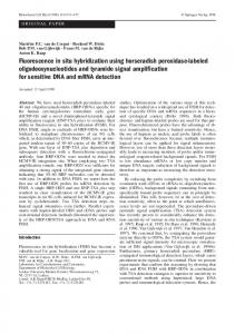
Figure 19: Absorbance spectra of a 5% weight per volume solution of holmium oxide in 1.4 N perchloric acid (BDH Chemicals) measured using a Perkin Elmer Lambda 25, Perkin Elmer Lambda 2 and NanoDrop averaged over 3 measurements. The accepted wavelengths are 241.1±0.1, 249.7±0.1, 278.7±0.1, 287.1±0.1, 333.4±0.1, 345.5±0.1, 361.5±0.1, 385.4±0.2, 416.3±0.2, 450.8±0.2, 452.3±0.2, 467.6±0.2, 485.8±0.2, 536.4±0.2, 641.1±0.2, 891±1, 1159±1 and 1190±1 n m respectively [97,98]. The working range of the Lambda 2 and 25 is between 190-1100 nm meaning the last 2 peaks could not be measured on the Lambda 2 and 25. The monochromators were stepped in 1 nm increments with a 0.125 s integration time. The NanoDrop 2000c was ran over its working range 190-840 nm using a 5 s integration time. This meant the last 3 peaks could not be measured on the NanoDrop. Since the Lambda 2 and Lambda 25 were stepped in 1 nm increments and the NanoDrop 2000c has a 1.8 nm spectra resolution the 2 peaks at 450.8 nm and 452.3 nm are indistinguishable and so only one peak at 451 nm was measured. The results for all instruments are in good agreement to the accepted values however since the NanoDrop is designed for higher absorbance samples it yields slightly noisier data than the Lambda 2 and 25.
26
A number of standards may be made up to predetermined concentrations with spectroscopic grade solvent to assess the linearity of the spectrophotometer, the preferred choice for a spectrophotometer characterisation is usually potassium dichromate in 0.001 M perchloric acid [99,100]. Strictly speaking fluorescent standards are less preferred for a spectrophotometer characterisation however as this work is more focused on fluorescence spectroscopy Rhodamine 6G which has an extinction coefficient of 10.5×10⁻⁴ mol–1 L cm1
in ethanol at 530 nm according to supplier data [77]. Rhodamine 6G [101] solutions of 10
known concentrations were made up which had absorbance values made up between ~0.010.10 Figure 20. The extinction coefficient was measured to be =(10.66±0.04)×104 mol–1 L cm–1 with R2=0.9999 in a Perkin Lambda 25 spectrophotometer and =(10.63±0.04)×104 mol–1 L cm–1 with R2=0.9998 in a Perkin Elmer Lambda 2 spectrophotometer. Results are in good agreement to literature values. The same samples will later be used to test the linearity in a fluorimeter.
Figure 20: The absorbance spectra of Rhodamine 6G in ethanol measured using a Lambda 25 at low concentrations. The scan was run from 350-650 nm in 1 nm steps with a 0.125 s integration time was used. Data was baseline corrected and the peak absorbance was measured to be at 530 nm and observed to be linear with respect to concentration. A linear fit gave an absorption coefficient of =(10.66±0.04)×104 Mol–1 L cm–1 with R2=0.9999. The Lambda 2 gave similar data with an absorption coefficient of =(10.63±0.04)×104 Mol–1 L cm–1 with R2=0.9998.
27
2.1.2 Transmission of Optical Components and Filters It is insightful to check the transmission spectra of any optical components used for experiments such as longpass Figure 21, bandpass and neutral density Figure 23, Figure 24 filters as well as cuvettes Figure 22 [102] and polarizers. Transmission spectra are usually supplied with such components making verification of the spectra a good test for the spectrophotometer. It is also important to get a good understanding of the optical components utilised as well as their working range. Absorbance and fluorescence data measured outside a component’s working range is often meaningless. As the transmission spectra of such components should be constant they may also be used to quickly diagnose any defects in the spectrophotometer. In addition to the optical components mentioned above it shouldn’t be forgotten that solvents likewise have an optical effect and an associated working transmission range [102,103]. The transmission spectra is also a useful check for the alignment of the system particularly the alignment of a beam when using specialised micro-cuvettes for low volumes [104]. The spectrophotometer is a useful instrument to check the transmission properties of optical components and the absorbance spectrum can be used to determine an analyte and give a measure of an analytes concentration as shown in Figure 20.
Figure 21: The transmission spectra of the longpass filters inventory measured using a Perkin Elmer Lambda 25 spectrophotometer ran from 200-1100 nm in 1 nm increments. A 0.125 s integration time was used. Longpass filters are usually characterised by the wavelength where they attenuate the wavelength by 50 %.
28
Figure 22: The transmission spectra of cuvettes inventory measured using a Perkin Elmer Lambda 25 spectrophotometer ran from 200-1100 nm in 1 nm increments. A 0.125 s integration time was used. The transmission spectra of a PMMA UV grade, which is stated to have a usable range of 280-900 nm, of a glass cuvette which is stated to have a usable range of 334-2500 nm and of a quartz cuvette which is stated to have a usable range of 1702700 nm measured using a Perkin Elmer Lambda 2.
Figure 23: The transmission spectra of Schott Neutral Density filters measured using a Perkin Elmer Lambda 2 spectrophotometer ran from 200-1100 nm in 1 nm increments. A 0.125 s integration time was used. The spectra match those provided by the supplier and demonstrate that these components are unsuitable for measuring in the UV region and work optimally between 400-650 nm region.
29
Figure 24: The transmission spectra of UV Metallic Neutral Density filters provided by the supplier which demonstrates that these components are suitable for measuring in the UV region right through to the NIR regime. 2.1.3 Limitations Absorbance spectroscopy however has two limitations the first is of sensitivity. The analyte measured Rhodamine 6G is a dye with an extinction coefficient=(10.66±0.04)×104 mol– 1
L cm–1. Many analytes that one would wish to investigate in particular biological
molecules such as proteins will have an extinction coefficient significantly lower. Moreover, proteins are considerably larger that dye molecules like Rhodamine 6G and hence have a large cross-section which enhances Rayleigh scattering. Figure 25 illustrates the problem of Rayleigh scattering with absorbance spectra. LUDOX SM-AS is a silica nanoparticle with 𝑅 = 3.5 nm and is commonly used in fluorescence measurements to make a scattering solution. The increase in measured “absorbance” as the concentration of scattering solution increases is due to scattered light and not from actually absorbance of LUDOX SM-AS. Scattered light has a –4 dependence [105] and hence distorts the UV regime the most. It should be noted that the relationship between the quantity of scattering specie in this case LUDOX SM-AS and the magnitude of the absorbance is clearly nonlinear. Biological molecules such as proteins typically have an absorbance spectrum in the UV but may also highly scatter making it difficult to separate out their actual absorbance spectra. In general, for the same material the larger the size of the nanoparticle, the more intense the scattering. This phenomenon is taken advantage when using light scattering techniques such as Nanoparticle Tracking Analysis (NTA) on nanoparticles >50 nm [106,107]. Finally, absorbance has the limitation of sensitivity, in the Perkin Elmer Lambda
30
2 and Perkin Elmer 25 used it is hard to accurately measure below A~0.01 for a 1 cm path length due to the difficulty in accurately distinguishing small differences in two relatively large signals. Sensitivity can be helped slightly by use of longer path length cuvettes.
Figure 25: “Absorbance” of LUDOX SM-AS solutions in distilled water measured in a Perkin Elmer Lambda 25 spectrophotometer ran from 230-500 nm in 1 nm increments. A 0.125 s integration time was used. In each case the volume of LUDOX SM-AS stated in the legend was added to 3 ml of distilled water.
This is illustrated in Figure 25 with the 0 µl control i.e. distilled water where an absorbance of –0.006 is measured at 240 nm. In the case of a biological molecule such as a protein there is problem of a lower extinction coefficient e.g. 43824 mol–1 L cm–1 [108] and a practical limitation of measuring absorbance values below 0.01. For a 1 cm cuvette using Equation (18) it will be hard to accurately measure the µM range and the nM range certainly is out of reach. On the other hand, high absorbance values are difficult to measure accurately because of non-linear effects such as scattering. Fluorescence techniques on the other hand are boasted of being capable of measuring concentration values of up to one million times smaller than absorption techniques [109] with up to pM sensitivity being reported [110].
31
2.2 Emission – Spectrofluorimeter
Figure 26: The excitation optics of the spectrofluorimeter are similar to that of a spectrophotometer consisting of a xenon arc lamp, excitation monochromator and sample compartment. The detection optics differ in the fact that they are situated at right angles from the excitation arm13 and there is an additional monochromator to select emission wavelength14. If polarization effects are present, excitation and emission polarizers may also be present. The monochromators are drawn in Czerny-Turner geometry. Fluorescence techniques can use extremely low amounts of fluorophore (µM-nM concentrations) which is important to minimised perturbation of the system under investigation particularly in the application area of the life sciences. The steady state fluorescence properties of a sample may be investigated by usage of a spectrofluorimeter.
13
Fluorescence occurs in all directions and is much weaker than the excitation signal. The right angle conformation is used to reduce the proportion of excited light to fluorescence emission. In addition, the xenon arc lamp is typically much more powerful than the deuterium and halogen lamps used in a spectrophotometer. 14 The detection wavelength is typically different to the excitation wavelength unlike in the spectrophotometer.
32
As fluorescence spectroscopy involves looking at an emission signal with a low background level that is Stokes shifted in wavelength from the excitation source, fluorescence can be as much as 1000 times more sensitive than absorption spectroscopy which in contrast involves looking at comparing two relatively large signals which will be very similar at low absorbance values. The excitation optics are similar to the optics of a spectrophotometer15 however in general a more intense excitation source is used because the fluorescence signal is typically orders of magnitude less than the excitation light. The excitation source is a 450 W Xenon lamp for the modular Fluorolog 3 and a 150 W Xenon lamp for the benchtop Fluoromax. Two single grating monochromators are drawn in Figure 26 which is the standard configuration for the Fluoromax 4 and the basic configuration for the Fluorolog 3 (Fluorolog 3-11). Blazed gratings are manufactured to produce maximum efficiency at certain wavelengths. Typically, a grating blazed for a lower wavelength is used for the excitation to maximise the relatively low output of the Xenon lamp than the emission which is typically measured at higher wavelengths. For example, a grating with 1200 lines/mm blazed at 330 nm may be used for excitation and a grating with 1200 lines/mm blazed at 500 nm may be used for emission as shown in Figure 27. For optimal results [111]:
2 Blaze 0.4 is due to glycerol Raman scattering. The anisotropy is close to 0.32 in all regimes of interest (where the Rhodamine 6G fluorescence is strong) meaning the excitation and emission dipoles are close to parallel and any wavelength pair where the fluorescence of Rhodamine 6G is strong is a good place for anisotropy measurements.
Figure 75: The steady-state fluorescence anisotropy of Rhodamine 6G with respect to increasing percentage of glycerol solution measured in a Fluorolog 3-22 with a R928 PMT. The excitation monochromator (1200/330 double grating) was set to 532 nm with a 5 nm bandpass. The emission monochromator (1200/500 double grating) was set to 570 nm with a 5 nm bandpass. For each excitation, emission wavelength pair 4 measurements were carried out with 4 different polarizer orientations VV, VH, HV and HH respectively. A 2 s integration time was used for each polarization with a maximum of 25 trials (set to get a standard deviation of 5 %). As the viscosity increases, the Brownian motion of Rhodamine 6G slows down and a higher anisotropy is reported.
90
2.3 Time Resolved Emission – Spectrofluorometer Unlike the fluorescence intensity which is usually expressed in arbitrary units, the fluorescence lifetime is an absolute number derived from a histogram. The fluorescence lifetime isn’t distorted to the same extent as raw intensity measurements are with innerfiltering effects or by photobleaching [178]. The fluorescence lifetime of a fluorophore can be tailored to be extremely sensitive or robust to changes in its local environment which may be due to the presence of a specific analyte for example. In many texts the fluorescence lifetime is quoted as independent of the fluorophore’s concentration. This assumption is only valid providing the appropriate concentration regime for fluorescence measurements is adhered to27.
Figure 76: Illustration of the time-scale of Rayleigh scattering at the wavelength of the excitation source. At longer wavelengths there may be weak Raman (Stokes) scattering and the processes that are of the most interest, fluorescence and phosphorescence. These processes may be distinguished via measurement of their time scale.
Lifetime is often quoted as being independent of intensity. Care should be taken with this statement as it’s only true within the small concentration regimes typically used for fluorescence measurements. Too much fluorophore will change the environment and hence the fluorescence lifetime. If the fluorophore is part of a large structure for instance a decrease in lifetime may occur due to increased collisions and an assortment of energy transfer mechanisms between fluorophores. 27
91
In sensing applications the fluorescence intensity and the fluorescence lifetime may both be used in conjunction to infer the concentration of an analyte however the fluorescence intensity may decrease over time due to photobleaching and hence erroneously reporting a lower analyte concentration whereas the fluorescence lifetime on the other hand as an absolute number will remain consistent [17]. The change in the fluorescence lifetime can therefore act as a far more accurate sensor. In the introduction the time scale of both scattering phenomena and photoluminescence was discussed, these processes have differing time scales; Rayleigh (elastic scattering) ~fs, Raman (inelastic scattering) ~fs-ps, fluorescence ~ns and phosphorescence ~µs-s. The fact that these processes have a different time-scales is of great importance to time-resolved measurements and is routinely taken advantage of. It is possible to separate out these processes by using time as an additional axis as demonstrated later. The optics of instrumentation for time-resolved fluorescence is unsurprisingly similar to that of steady-state fluorescence counterpart; the main difference is the excitation source is pulsed in a time interval which is ideally much shorter than the fluorescence decay time of interest and the system needs to incorporate timing electronics sufficiently fast enough to detect the decay. Monochromators which have less surfaces are usually preferred for optimal time-resolution so a dedicated system is preferred opposed to a hybrid. As the light sources used for fluorescence lifetime measurements are already monochromatic an excitation monochromator is not usually required. Timing electronics are added to count the difference between the start (light source) and stop (detector) pulses. In the HORIBA Scientific DeltaPro and TemPro there are no emission or excitation monochromators and the separation of the fluorescence emission from the excitation is solely controlled by the right angle orientation and use of a series of longpass or bandpass filters as shown in Figure 21. Such a configuration is extremely useful for weak signals providing the sample doesn’t scatter too much. The steady-state fluorimeters such as the HORIBA Scientific Fluorolog or Fluoromax can be upgraded with the pulsed light source and timing electronics to become a HORIBA Scientific Deltatime hybrid systems. Mainstream light sources employed for time resolved fluorescence are discrete lasers and diodes.
92
Figure 77: The optics of a time-resolved spectrofluorometer are very similar to steady-state counterpart the spectrofluorimeter. In this case the monochromators are drawn in SeyaNamioika geometry which is typical for the HORIBA Scientific DeltaFlex, FluoroCube and Ultima systems. The light source28 is usually a laser diode or diode of discrete wavelength such as the HORIBA Scientific DeltaDiode and NanoLEDs or the SpectraLEDs for phosphorescence measurements. The detector is usually a TBX650/TBX850c for FluoroCube systems, a PPD-650/TBX850c for DeltaFlex systems or a Precision Photomultiplier MCP for Ultima systems. In such a configuration there is no XCorrect correction factor and no ability to measure an excitation spectrum. Laser diodes and diodes are much more stable in output than the xenon arc lamp so there is usually no need to divide by a reference when using them for a kinetic measurement.
28
The light sources will be denoted DD, NL and SL for a DeltaDiode, NanoLED and SpectraLED respectively. Next the wavelength will be denoted as xxx and then L or D will be added to denote a laser or a diode. For example, a DeltaDiode laser with a peak wavelength at 503 nm will be called DD503L.
93
Figure 78: Addition of timing electronics DeltaHub and TB02 and a pulsed light source DeltaDiode/NanoLED/SpectraLED to a HORIBA Scientific Fluorolog 3-22 to form the HORIBA Scientific Deltatime system29. The xenon lamp is switched off during operation of the pulsed light source. In a few extremely high end systems a super-continuum laser is used as a light source, for example in the Fluorolog Extreme where the xenon arc lamp is replaced by a NKT supercontinuum laser and timing electronics are added between the light source and the detector. Also in the DeltaFlex Extreme where the excitation monochromator and NKT laser is used as an excitation source. Although the NKT super-continuum laser may appear to be the best light source regarding dynamic wavelength range, it should be noted it misses a substantial proportion in lower end of the visible range and UV range which are used for an assortment
29
Note for fluorescence lifetime measurements a double grating monochromator is not as efficient as a Time Domain Monochromator. The number of surfaces the emission beam has to interact with on a double grating monochromator is increased making the wavelength time-spread larger thus it is harder to resolve smaller decay times. Deltatime systems typically invoke a single grating monochromator in a T format e.g. Fluorolog 3-211 (not shown) to reduce the number of surfaces. This configuration has a lower time resolution than a dedicated time-resolved system such as a DeltaFlex and certainly an Ultima.
94
of fluorescence measurements. Moreover, it has limitations in the number of repetition rates and this hence limits its overall usability in the number of time ranges where it can be employed. Its output per wavelength may be significantly lower than the DeltaDiode lasers. As the work in this thesis was carried out in conjunction with HORIBA Scientific multiple development spectrofluorometers of varying configurations were employed. Previous generations of hardware include the HORIBA Scientific FluoroCube and HORIBA Scientific TemPro systems with HORIBA Scientific Hub A and inbuilt NanoLED controller. The timing electronics incorporated the FastComTech MCA-3 and National Instruments NI-6602 PCI cards. For TCSPC the best time-resolution per channel is ~7 ps ch–1 or 0.7 ps ch–1 with a time expander and the electronic deadtime is ~1 µs. NanoLED light sources can be pulsed from 10 kHz to 1 MHz. For MCS the maximum time-resolution per channel is 500 ns ch–1. To accommodate the timing electronics a custom computer was built and the latest release of DataStation was installed. State of the art HORIBA Scientific DeltaFlex and DeltaPro systems were used with DeltaHub and DeltaDiode electronics. The best time-resolution for TCSPC is slightly higher at ~13 ps ch–1 however the instrument deadtime is 10 ns, a factor of 100 less than previous instrumentation moreover DeltaDiode light sources can be pulsed from 10 kHz-100 MHz. The low deadtime of the DeltaHub in combination to the higher repetition rates of the DeltaDiodes significantly speeds up data acquisition on smaller time ranges making these high-throughput systems [179] and hence widen the application area which is important for applications such as enzyme kinetics. For MCS the maximum resolution is ~85 ns ch–1. For DeltaHub electronics no special cards are required so a standard computer was used with the latest release of DataStation. The DeltaFlex and FluoroCube may or may not have an excitation monochromator; the reason for omitting the excitation monochromator on these systems is that typically excitation sources such as laser diodes or diodes are used which have a defined wavelength and hence all an excitation monochromator will do is attenuate the signal. Although a supercontinuum laser with an excitation monochromator would apparently make a more versatile system, it is not as cost-effective as multiple laser diode sources and the output may be significantly lower at some wavelengths with no output in the UV range. The DeltaPro and TemPro systems are systems without any monochromators and typically one or more long pass filters are used to select the emission wavelength, although these systems aren’t as versatile as the DeltaFlex and TemPro systems they can have the advantage when measuring samples with weak fluorescence emission.
95
2.3.1 Measuring a Long Lived Phosphorescent Fluorescence Decay with Simple Electronics A long lived phosphorescence decay such as the emission from lanthanides [180] of the order of 0.1 ms may be recorded in a multitude of different ways, some more efficient than others. A sparked light source such as a xenon flash lamp may be used as a relatively cheap excitation source covering a vast range of wavelengths. A PMT is typically used as a detector; CCDs are in general not fast enough for phosphorescence decays. The phosphorescent decay may be obtained by using simple electronics. Figure 79 and Figure 81 demonstrate measuring a fluorescence decay using the decay by delay and decay by window methods accordingly. In the decay by delay protocol an initial delay is set after the lamp pulse and a measurement window with a fixed integration time is utilised. The xenon lamp is flashed and the number of photons within the measurement window is recorded. The measurement window is then moved by a specified delay increment, the xenon lamp is again pulsed and the number of photons measured is again recorded. This continues until the desired range is scanned. Normally the lamp is told to flash 1-999 times per delay interval. Just like steady-state measurements one has to ensure that the detector is working in its linear range. The maximum number of counts per measurement:
Linear Range of PMT No of Flashes (48) tWindow where the linear range of the detector is taken from the specification sheet in CPS. The No of Counts Max
window integration tWindow time is taken in s and the no of flashes is dimensionless. If the number of counts > No of CountsMax the earlier windows which should have the most counts i.e. the start of the decay will experience photon pile-up Figure 80. Later windows where the long lived fluorescence/phosphorescence has significantly decayed won’t have as many counts and hence won’t experience pile-up. As pile-up essentially reduces the collection efficiency of the detector at shorter channels, the decay will be biased to longer decay times. For this type of measurement, the minimum feasible window integration time is about 5 µs. The initial delay is usually set to greater than 50 µs to ensure that there is no distortion on the measured long lived fluorescence/phosphorescence decay caused by the lamp profile, direct exponential fits of the decays can be used after the initial 50 µs. This method is good for crude measurements of long phosphorescence decay times. Measuring a fluorescence decay using this type of measurement and pushing for superior time resolution and hence better statistics is possible, but the cost comes at the data-acquisition 12 hours to acquire. The measurement of the decay by window shares the same limitations.
96
Figure 79: In the decay by delay, the time per flash and number of flashes per point are prescribed. An initial delay is set and a fixed sample window is specified. The delay is then increased by the specified increment and the number of counts within the measurement window is recorded. This continues until the maximum delay prescribed is reached.
97
Figure 80: Schematic to illustrate pile-up in the Delay by window method. Under the correct measurement conditions (left) each window will have a photon count rate within the linear regime of the detector. Figure 47 depicts the non-linear response of the detector at higher count rates and the switching off of the detector at extreme count rates. When out with the linear regime (right) early windows will have a count rate which exceeds the linear regime of the detector and as a consequence the counting efficiency will drop significantly. Medium windows will experience slight pile-up conditions and experience a diminished counting efficiency although to a lesser extent. Later windows will not experience pile-up and have standard counting efficiency. Comparing the ratios of heights Early:Medium:Late on the left versus the right the net effect is to bias the decay to longer decay times.
98
Figure 81: In the decay by window, the time per flash and number of flashes per point are prescribed. An initial delay is set and fixed; the minimum sample window is then specified with a windows increment. The windows increment is then increased by the specified increment and the number of counts within the measurement window is recorded. This continues until the maximum delay prescribed is reached. 99
Figure 82: Phosphorescence decay of aqueous europium chloride made to an absorbance of 0.1 measured in a Fluorolog 3-22 with R928 PMT. A xenon flash lamp was used as an excitation source. The excitation monochromator (1200/330 grating) was set to 392 nm with a bandpass of 5 nm and the emission monochromator (1200/500 grating) was set to 590 nm with a bandpass of 2 nm. The phosphorescence decay of the 5D0→7F1 transition is ≈110 µs [181]. This was setup using the internal electronics in the decay by delay operation. The time per flash was set to 41 ms (the maximum repetition rate for the Xenon Flash lamp is 25 kHz) and a flash count of 100. Top the initial delay was setup at 50 µs with a sample Window of 20 µs and a decay increment of 20 µs was used until the maximum delay of 2 ms was reached. This gave a mono-exponential decay time of 111±3 µs with a 2=1.340 and took approximately 10 minutes to acquire. Bottom the system was pushed to its limits with a flash count of 999. The initial delay was setup at 1 µs with a sample Window of 5 µs (the smallest Window size with a large enough number of counts over the background noise). In order to look at the decay in more detail an increment of 2 µs was used until the maximum delay of 2 ms was reached. This gave a mono-exponential decay time of 111.2±0.9 µs with a 2=1.064. This measurement took 12 hours acquisition time!
100
2.3.2 Multi-Channel Scaling (MCS) A multi-channel scaler can be considered as a series of single photon counters, with one counter for each data-channel in the decay trace. The timing electronics of the DeltaHub can use MCS with a time-resolution of ~85 ns ch–1 while the MCA-3/NI6602 cards in the Hub A have a maximum resolution of 500 ns ch–1. MCS is a more direct measurement of the fluorescence decay. The timing electronics of a MCS are far superior to that of the xenon flash lamp natively. Apart from the advantage of time resolution the main advantage is that the entire long lived fluorescence/phosphorescence decay is captured by the electronics in a single sweep of the multi-channel scaler. In comparison to the decay by window method, a multi-channel scaler can be thought as up to four thousand windows side by side known as channels Figure 83.
Figure 83: Concept of MCS with respect to the decay by delay method. 4000 windows (channels) are placed side by side and the entire decay is obtained in a sweep. A series of sweeps are measured until the desired peak preset or time preset is reached. In a MCS measurement, a peak preset or time preset is usually set in order to achieve the desired number of counts. The advantage of MCS compared to the decay to delay window is illustrated when comparing Figure 84 to Figure 82, which is the same sample, measured 101
in the same instrument with and without DeltaHub electronics. The measurement with the DeltaHub electronics uses MCS, has a higher time resolution, and takes 15 minutes, the measurement without the DeltaHub electronics has a worse time-resolution and takes 12 hours to measure. The DeltaHub in the case of this sample therefore leads to a 100-fold increase in throughput while achieving superior time-resolution. Pile-up conditions will affect the channels with the most counts in exactly the same manner as the decay by delay measurement type. In order to avoid pile-up for a MCS measurement the number of photons recorded is typically attenuated with neutral density filters to be less than 2 % of the start rate where necessary.
Figure 84: Phosphorescence decay of aqueous europium chloride made to an absorbance of 0.1 measured in the same Fluorolog 3-22 with a R928 PMT. The optics were setup identical to Figure 83 however a DeltaHub was used to measure the phosphorescence using multi-channel scaling with a time range of 2.7 ms and peak preset of 10,000 counts. This gave a time calibration of ~667 ns ch-1 and measured to a peak preset of 10,000 counts in 15 minutes. This gave a mono-exponential decay time of 111.7±0.3 µs with a 2=1.041. HORIBA Scientific SpectraLEDs typically have a broad ~30 ns pulse. Although they are of discrete wavelengths, SpectraLEDs are better excitation sources for phosphorescence measurements and do not possess an afterglow which may be present in some Xenon Lamps [182]. When using SpectraLEDs for a MCS measurement there is the ability to
102
select an optional delay30 and duration of continuous excitation; the continuous excitation allows the sample to reach a steady-state which may not be achieved in the time of a xenon lamp flash31. After continuous excitation the light source is switched off and the fluorescence decay is recorded. The form of a MCS recorded with a SpectraLED is characteristic of Figure 85; initially it takes some time to excite the sample so there is a lag at the start until the sample has reached steady conditions i.e. the plot is flat. After continuous
excitation
the
SpectraLED
is
turned
off
and
the
long
lived
fluorescence/phosphorescence decay is recorded.
Figure 85: MCS phosphorescence decay of aqueous europium chloride made to an absorbance of 0.1 measured in a DeltaFlex hybrid using a SL373D as an excitation source. The emission monochromator TDM800 (1200/350 grating) was set to 590 nm with a bandpass of 2 nm. A TBX850c was used for detection. A DeltaHub was used to measure the phosphorescence using multi-channel scaling using a time range of 5.4 ms and a peak preset of 10,000 counts. This gave a time calibration of ~ 1333 ns ch-1 and measured to a peak preset of 10,000 counts in 30 minutes. A delay of 10 % the time range was selected (a) then the SpectraLED was turned on. The emission from the sample takes some time (b) to reach steady state (c). In this case the SpectraLED was turned on for 25 % of the time range (b+c). The phosphorescence decay is observed after the SpectraLED is turned off (d). The end of the decay (e) should be flat and of equal height to the start of the decay (a). This gave a mono-exponential decay time of 116±5 µs with a 2=1.249.
30
As a guide the optional delay is usually selected to be about 10 % of the time range and used as a check to ensure the noise level at the start and end of the time range is flat i.e. that there is no longer lived component present. 31 The sample does not need to reach this steady state condition but this condition ensures the maximum number of photons per sweep and hence minimises the acquisition time.
103
DeltaDiode lasers can also be used as a source for MCS. Like the SpectraLED an initial delay can be set. Then the DeltaDiode can be pulsed at 80-100 MHz32 for a period of time. Finally, they can then be switched off to measure the decay. When measuring a phosphorescence decays care needs to be taken in order to avoid re-excitation of the sample before the decay completes, failure to do so will result in a non-linear background before the decay and after the decay.
Figure 86: A MCS measurement of Tb in glass (IBH test sample) using a DeltaFlex with a SL373 excitation source and with an emission monochromator TDM800 (1200/450 grating) at 545 nm with a 12 nm bandpass. The DeltaHub timing electronics were used with a PPD850 detector. A peak preset of 10000 counts was selected. The SL373D is ran with a 10 % delay and 10 % duration for each time range. When the time range of 44 ms is used a complete phosphorescence decay is observed, the background noise before the decay is flat this regime is shown in the bottom graph in more detail. As the time range of 32
At the large time-ranges MCS operates this can be considered as continuous excitation.
104
measurement is increased the background before the decay is observed to increase and the background is no longer flat. This is because the phosphorescence decay has not fell to zero from the previous sweep before the next sweep is initiated. To an untrained eye this may be mistaken as high dark counts. 2.3.3 Time Correlated Single Photon Counting Principle Current timing electronics are not fast enough to directly measure the complete fluorescence decay in the ns time-range because of the significant deadtime of timing electronics which can often be many orders of magnitude larger than the lifetime of a fluorescence decay for older electronics. Figure 87 illustrates the bias to shorter decay times because photons arriving at the detector during the electronic deadtime are not detected. Time Correlated Single Photon Counting (TCSPC) is an indirect measurement of the fluorescence decay. With TCSPC the hit rate that is the ratio of Stop/Start pulses is usually constrained to 2 %. For low deadtime electronics this limitation can be relaxed to 8-10 %. In practice this is carried out use of neutral density filters for strong samples c.f. Figure 23 and Figure 24. The timing electronics which can be thought of as a sophisticated stop watch Figure 88 with three buttons. The constraint of the hit rate means that for the majority of measurements the timing electronics will Start and no photon will be detected, the end of the time range will be reached and then the system will Reset. After a Reset one must wait for the system deadtime to pass before beginning the procedure over and over
Figure 87: The sample is excited by a -pulse and a photon D(1) is detected. After this photon is detected the timing electronics are reset. During this reset time otherwise known as deadtime no detections are possible. A second photon arriving at this time is thus
105
undetected UD(2). If this procedure continues the measured decay is extremely biased to shorter decay times.
Figure 88: The timing electronics can be thought of as like a stop watch with three buttons. Start, Stop and Restart. In single photon counting mode, the stop/start ratio is constrained to prevent detection and timing of a single photon and the failure to detect a second photon during the system’s deadtime. This constraint means that in the bulk of cases the system will start timing (1st frame), the time of the Start will be recorded (2nd frame) and no photon will be detected. The systems electronics will then reset (3rd frame) and then the system will have to wait on the deadtime until it can begin the entire process again (4th frame) [183,184].
106
Figure 89: The timing electronics can be thought of as like a stop watch with three buttons. Start, Stop and Restart. In single photon counting mode, the stop/start ratio is constrained to prevent detection and timing of a single photon and the failure to detect a second photon during the system’s deadtime. This constraint means that only in some cases the system will start timing (1st frame), the time of the Start will be recorded (2nd frame) and a photon will be detected (3rd frame). The microscopic time (time between the start and stop) and in some cases the macroscopic time (time from the start of the reaction) will be stored. The systems electronics will then reset (4th frame) and then the system will have to wait on the deadtime until it can begin the timing process again [183,184].
107
again. In a small fraction of the timing cycles a photon will be detected leading to a Stop. The microscopic time that is the time between the start and stop is stored and in some cases the macroscopic time, that is the time from the start of the measurement is stored. After a Stop the timing electronics Reset and again one has to wait on deadtime before it can begin timing again. Like MCS the time range consists of a number of channels and each channel is assigned a finite time width. A histogram is built up to a designated peak preset typically 10,000 counts or a designated integration time preset. 2.3.4 Instrumental Response Any fluorometer will have its own instrumental response; the instrumental response is brought about by the fact that the excitation pulse is not a -pulse and may also be broadened from imperfections in both the electronic [185] and optical [173] components. The main limitation is the non-linear detector response which is brought about as a result of the transit time spread of the photomultiplier [186–188]. This instrumental response must be measured in order to extract meaningful data for short time ranges. Rayleigh scattering is of the order of (~10–15 s) and thus with the respect to the response of a time-resolved fluorometer can be thought of as instantaneous. By measuring Rayleigh scattering one can hence get a measure of the instruments response. The instrumental response of the system or prompt is typically measured using a dilute colloidal solution usually LUDOX SM-AS which will be examined in more detail later. When measuring the prompt the emission monochromator is set to the excitation wavelength and both polarizers are set to the vertical orientation (if present). These conditions are optimised to measure Rayleigh scattering33
Figure 90: Typical polarizer and monochromator conditions for the scatter or prompt measurement. If an unpolarised Diode is used as an excitation source, polarizers aren’t required. 33
VV polarizer configurations are used for the Prompt as Rayleigh scattering is fast and hence the most prominent in the VV orientation.
108
and to minimise the effects of fluorescence. The instrumental response from a Xenon lamp may be quite broad due to the profile of the Xenon flash lamp. In this case a FWHM ~0.5 µs was recorded using MCS, this is negligible compared to the 116 µs decay time measured in Figure 82 and Figure 84 which was satisfactorily tail fitted. Clearly however this type of light source is not suitable for ns decay times.
Figure 91: The time-profile of the xenon flash lamp measured on a Fluorolog 3-22 with DeltaHub and R928 PMT. The excitation monochromator (1200/330 double grating) was set to 392 nm with a 3 nm bandpass. The emission monochromator was set to 392 nm with a 3 nm bandpass. A dilute LUDOX SM-AS solution was used as a scattering solution. The maximum time resolution for MCS was utilised ~85 ns ch–1. The DeltaDiode, diode sources typically have a FWHM~750-1000 ps for example DD280D and DD295D. Such pulses have quite a smooth appearance when measured with modern electronics see Figure 92. DeltaDiode sources also have a monochromatic output; the second peak observed is due to second order effects of the monochromator which allow some excitation light to reach the detector. It should be noted that this can be prevented in fluorescence measurements by the addition of a long pass filter of appropriate wavelength. Laser sources on the other hand can have a much smaller instrumental response which can fall into the ps or even fs regime. However the transit time spread of the photomultiplier for example in the TBX650/PPD-650 and TBX850c/PPD-850c picosecond detection modules are ~180-250 ps [137]. The prompt of DD405L has a FWHM of ~200 ps with the TBX850c. The appearance of the prompt shows a second peak which is an artefact due to 109
the non-linear transit spread time of the detector. This afterpulse is caused by the elastic scattering of electrons off the first dynode c.f. Figure 48 [189,190]. In order to overcome this problem and to accurately to measure decay curves at small time ranges re-convolution analysis must be applied which will be discussed later. It should be noted that extremely old TBX picosecond detection modules may also exhibit later after-pulses. All these afterpulses will also be taken into account when re-convolution analysis is used. If the system is not very aligned or additional optics are used additional peaks may appear in the instrumental response due to reflections Figure 94. When a light source is swapped with another source of differing wavelength or the cuvette holder is swapped the system should be checked for alignment and the focusing optics should be optimised using a Focus Scan. The effect of the broadening of Rayleigh scattering from the DD405L (Rep Rate=20 MHz) by detector response and electronics may be seen by plotting both a prompt measured with a Hub A/MCP system alongside a prompt measured with a DeltaFlex/PPD850 Figure 96. Care must be taken when using the MCP as it has a lower dynamic range than other PMTs (50000 CPS opposed to 2000000 CPS) and if the number of counts is too high the pulse will broaden. The timing electronics of the Hub A and MCP must be given some time to stabilise after powering on otherwise the pulse will likewise broaden. Optical alignment and reflections are more significant when trying to get a fast pulse on a MCP system. Measurement of the DD405L on the MCP systems shows that the instrumental response is limited by the laser profile. The laser profile is significantly faster than the Diode or Xenon flash lamp but it takes some time for the electronics to switch off the laser which is measurable on a MCP system.
110
Figure 92: Steady-state and instrumental response of DD295D (Rep Rate=20 MHz) measured on a DeltaFlex with a TDM800 (1200/350 grating) with a PPD850. For steadystate the emission bandpass is constrained to 2 nm and the monochromator is scanned at 1 nm increments over its entire working range the emission peak is found to be peak=294 nm with FWHM of 12 nm. For the time-profile the emission bandpass is opened to 12 nm and the time profile is measured to have a FWHM=768 ps at the peak wavelength. DeltaHub electronics are set to a time range of 100 ns (4000 channels). The monochromator when set to 592 nm allows second order emission of the excitation light; it should be stressed that this light is not the DeltaDiode lasing at 592 nm but the monochromator allowing light of 295 nm to reach the detector. The peak may be identified as second order because it resembles the 1st order peak but is lower in amplitude and is stretched out twice as wide. The 2nd order peak can be removed using a long pass filter alongside the monochromator. This was measured in a DeltaFlex34 with DeltaHub electronics and a PPD-850c. No additional ND filters were used and polarizers were removed. Diodes have a broad FWHM 34
In order to do this measurement on a FluoroCube with both an excitation and emission monochromator, the excitation monochromator may be set to 0 nm wavelength where it acts as a mirror.
111
and are unpolarised in output. A dilute LUDOX SM-AS solution was used as a scattering solution.
Figure 93: Steady-state and instrumental response of DD405L (Rep Rate=20 MHz) measured on a DeltaFlex with a TDM800 (1200/350 grating) with a PPD850. For steadystate the emission bandpass is constrained to 2 nm and the monochromator is scanned at 1 nm increments over its entire working range the emission peak is found to be peak=409 nm with FWHM of 3 nm. For the time-profile the emission bandpass is opened to 12 nm and the time profile is measured to have a FWHM=192 ps at the peak wavelength. DeltaHub electronics are set to a time range of 100 ns (4000 channels). As a laser is used polarizers were both at vertical orientation. The emission bandpass was set to 2 nm and to ensure that the counts were below 2×10⁶ CPS at the peak emission UV ND 2.0 and UV ND 1.0 were added to the excitation arm. It should be noted that the FWHM in this case is limited by the detector and not by the laser. A dilute LUDOX SM-AS solution was used as a scattering solution.
112
Figure 94: The focusing of optics is naturally important for the laser FWHM. The dashed line illustrates a badly aligned system. The solid blue line is the system focused scanned and the time delay changed slightly for clarity. (a) is the laser pulse of DeltaDiode on a 100 ns TAC range (4000 channels), (b) is an additional peak arising due to a reflection and (c) is the non-linear detector response.
Figure 95: In order to illustrate the effect of detector response in more detail. The same DD405L (Rep Rate=20 MHz) was measured using a HORIBA Scientific Ultima using the diode sync for optimum stability. This system has the Hub A electronics with the time expander enabled (0.701 ps ch–1) and a Precision Photomultiplier MCP [191] as a detector. In order to prevent the MPT from exceeding 50000 CPS 1 UV ND 2.0 and 1 UV ND 1.0 113
were used on each arm optic conditions were otherwise identical to Figure 93. Detector response is illustrated by measuring a prompt as soon as the detector is powered up and 15 minutes after it is stabilised. The FWHM was measured to be 67.0 ps and 41.3 ps respectively.
Figure 96: Artificial broadening of DD405L by the PPD850 can be seen by setting the peak of the prompt to 0 ns and plotting the prompts (Figure 94 and Figure 95) overlaid in time opposed to channels. It is insightful to see this in both log and linear scale. Now that the data is plotted with respect to time, the reflection can be discussed in more detail. Recall that the speed of light is 3×10⁸ m s–1 and in 40 ps, light travels 1.2 cm. This 1.2 cm is comparable with the size of the square sample compartment ~25 cm×25 cm. The reflection in the case of Figure 96 is measured ~1.25 ns after the main peak. This means light has travelled ~37.5 cm. In actual fact the reflected light has gone off in a diagonal bounced off the corner of the sample compartment and arrived at the detector 1.25 ns later. The overlay of both prompts shows the reflection measured at 1.25 ns in the case of the MCP would have been drowned out by the broadened detector response of the PPD850.
114
2.3.5 Delay lines, Repetition Rate and TAC Range A time range must be selected to suit the sample under investigation. Typically, the time range selected is 10-20 times the fluorescence lifetime of the sample. Samples usually have one decay time or multiple decay times of similar orders of magnitude so it’s usually an easy selection. The repetition rate is automatically selected when the NanoLED, DeltaDiode Laser or DeltaDiode Diode is coupled to the DeltaHub, Hub A or Hub B. NanoLEDs all have a maximum repetition rate of 1 MHz, DeltaDiode Diodes has a maximum repetition rate of 20 MHz and most DeltaDiode Lasers have a maximum repetition rate of 100 MHz. At factory the spectral and time FWHM of each source is measured using a system with a MCP c.f. Figure 92-Figure 95 and the power is measured using a power meter. Characterisation is carried out at various repetition rates to ensure the source passes or exceeds specifications. In order to obtain a complete fluorescence decay within a given time range the repetition rate of the light source has to be adjusted so that the following conditions are satisfied:
Max Rep Rate
1 Time Range
(49)
This is automatically selected in most cases however in some non-routine measurements a manual selection may be required. Samples which possess multiple species may include a very short decay time as well as a very long decay time. Adjustment of the time range to measure the long lived time component may give insufficient time-resolution to accurately measure the short lived component (there are a finite number of channels and these get stretched wider as the time range increased). In such complicated samples a short time range may be selected alongside a lower repetition rate in order to prevent sample reexcitation before the decay reaches noise35 c.f. Figure 86. The delay between the start and stop may have to be adjusted so the fluorescence decay is measured by an appropriate are of the TAC Figure 97. If forward mode is employed once the appropriate delay is set for the 100 ns time range, in general it doesn’t need to be altered if the time range is increased although there may need to be a slight adjustment for shorter time ranges.
35
In such complicated measurements the repetition rate should be lowered on the smaller time range to match the repetition rate that would be used in the larger time range in order to prevent re-excitation of the sample during measurement. The DeltaDiode can be disconnected from the DeltaHub to be manually controlled for such advanced measurements.
115
For the older MCA3/NI6602 systems however reverse mode is commonly employed in order to reduce measurement deadtime. When acquiring data at the short time ranges A tTAC=50-200 ns the deadtime of the timing electronics Hub A t Hub Dead =1 µs becomes
significant. For ease of calculation taking the 50 ns time range and 1 % hit rate as an example Figure 98. In forward mode one Starts the TAC with every excitation pulse. With a hit rate of 1 % only one of these excitation pulses leads to a detected photon thus in the vast majority of cases one measures for 50 ns and then Stops the TAC. With each Stop one has to wait 1 µs for the electronics to reset. The time to record a single photon is thus 100 × 50 ns + 100 × 1 µs ≈ 0.150 ms. In reverse mode one only Starts timing when a photon is detected and as the timing from the excitation pulse leading to this photon detection is not recorded, the time from this photon to the next excitation pulse is instead computed. The recorded data may then later be flipped so it appears like forward mode data using acquisition/analysis software. The time to record a single photon is thus reduced to 100 × 50 ns + 1 × 1 µs ≈ 6 µs.
Figure 97: Illustration of TAC Range and Delay adjustment for a mono-exponential sample. The TAC range is in generally selected to be 10-20 times that of the fluorescence lifetime. The top left illustration depicts a correct delay but incorrect TAC range, missing much of the decay curve. Because the repetition rate is also too high, before the prompt
116
part of a previous decay can be observed. The top right depicts again a correct decay but too large a TAC range, therefore less channels are used and the time resolution of the measurement is lowered. The middle left and right diagrams depicts a correct TAC range but too small and too large a decay respectively, missing much of the lifetime curve. The bottom left diagram depicts movement of the prompt with respect to the delay. Note time calibration of the TAC can be achieved by measuring the peak of the prompt with respect to the decay. The bottom right image depicts use of the correct delay and TAC range. Note the noise before the peak of the prompt is at the same level as the noise at the end of the decay meaning the complete decay has been measured and no re-excitation has occurred. In addition to the repetition rate the delay lines have to be adjusted so the fluorescence decay is observed within the measurement window. If the deadtime of the timing electronics is significantly larger than that of the time range being measured, reverse mode is commonly employed. In reverse mode the start and stop inputs are reversed so that the systems timing electronics measure the time between a detected photon and the next start pulse. The advantage of reverse mode is the timing electronics only “start” to measure for every photon detected opposed to every excitation pulse and hence there is no need to wait for the deadtime of excitation pulses, which do not lead to a detection. Taking a 1 % hit rate for example, data acquisition can be significantly speed up due to only having tDead opposed to 100tDead for every 100 excitation pulses. The fluorescence histogram is reversed compared to that traditionally measured in forward mode and additional delay lines may be required. The data can however easily be reversed in software and delay lines don’t affect the parameters obtained from the decay curve.
Figure 98: An illustration of forward mode operation vs. reverse mode operation where the time between the start and the stop tforward is the times recorded in order to obtain a decay histogram in forward mode. The time range tTAC and the system deadtime tDead are constant during measurement. It therefore follows that the time between the reverse start and stop 𝑡reverse = 𝑡Dead + 𝑡TAC − 𝑡forward . Due to the 1 % hit rate, the processes in the magenta
117
boxes occur 99 times for every photon detected whilst the processes of interest in the cyan box occur 1 time.
Figure 99: An illustration of how the delay on the stop moves the measurement window for reverse mode (data not reversed) and forward mode. A delay on the start will push the measurement window in the opposite direction. In both cases a delay is required to account for fine adjustments in system optics. In reverse mode the prompt should be present in the measurement window just before the Stop of the TAC. In forward mode the prompt should be present just after the start of the TAC. Data acquisition on screen is typically reversed when running in reverse mode so the decay curve looks like it is ran using forward mode. Reverse mode requires a delay on the Stop input approximately equal to that of the time range see Figure 99. For longer time ranges reverse mode is not applied due to the large delay required to move the prompt the full length of the time-range. The maximum delay that can be applied on the Start/Stop inputs of the Hub A is ~320 ns, if any more delay is added, the impedance is too high and the signal is lost however the advantage of reverse mode becomes less relevant as the system reaches a similar order of magnitude to the time range. The higher repetition rate of DeltaDiodes and low deadtime of the DeltaHub tDeltaHub =10 ns greatly increases throughput when short time ranges are employed. As the Dead deadtime is shorter or equal to the TAC range in all cases for the DeltaHub reverse mode is never used with the DeltaHub. The maximum repetition rate of the light source is inversely proportional to the time range used TCSPC becomes very inefficient at higher time ranges. For example, a 100 ns TAC range can utilise a fast repetition rate of 10 MHz but in practice is usually lowered to 8 MHz in case the time range is slightly larger than 100 ns and hence rapid acquisition of fluorescence decays can be achieved. Conversely the 13 µs TAC range can utilise a maximum repetition rate of 75 kHz, which in practice is usually constricted to 50 kHz in case the actual time range is slightly longer than 13 µs.
118
Data acquisition time can be substantially longer due to the use of the low repetition rate. Fortunately, the need for TCSPC diminishes at such time ranges because the timingelectronics become sufficiently fast enough to measure longer decays using more direct measurements such as Multi-Channel Scaling (MCS). The most time-consuming measurement is a measurement of a short decay and a long decay mixture where one wants to accurately resolve the short decay component and consequently has to use high time resolution but simultaneously lower the repetition rate of the laser to prevent re-excitation. 2.3.6 Time Calibration The time calibration per channel can drift over long periods of time especially in older systems which are capacitor based. In general, this drift is only significant for smaller time ranges, in particular, the 50-200 ns ranges and hence these time ranges should be periodically calibrated. A spectrofluorometers time calibration per channel can be measured using the prompt of a laser source with respect to variable delay lines or use of a TAC calibrator. For a quick calibration mono-exponential, lifetime standards can be prepared and used however care should be taken when comparing decay times from monoexponential standards to that of reference data as the decay times of reference data may be reported for N2 purged samples. This may hence lead to an incorrect calibration due to the large discrepancy between the decay times for samples measured without N2 purging and for those with N2 purging as demonstrated later in Figure 138. If a NanoLED is being used it should be given at least 30 minutes to stabilise before using it for a time calibration, as it needs to stabilise its temperature, DeltaDiodes on the other hand are temperature stabilised and can be hot-swapped. To make a calibration plot the channel of the peak of the prompt can be plotted with respect to the delay time as demonstrated in Figure 100 for the 50 ns range in a FluoroCube with a MCA-3/NI-6602 cards. Each time range used should be separately calibrated. Newer systems such as the DeltaHub have newer electronics which do not require user recalibration. The calibration can of course be checked with external delay lines. Using delay lines yielded a time calibration of 25.5 ps ch–1 which is in good agreement to the 26.0 ps ch–1 reported by the DeltaHub. The full width at half maximum FWHM measured in a DeltaHub however varies substantially more per channel and gives a higher fluctuation than that of the Hub A. This comes at the cost of the higher throughput. It should be noted that in most systems there is a finite number of channels therefore as the time range is increased, the time calibration per channel must also increase. Difficulty comes in measuring samples which exhibit both short decay times and long decay times 119
simultaneously; in order to measure the long decay time, the repetition rate has to be lowered and the time range has to be increased, lowering the time calibration per channel this clearly comes at the expense of the time resolution of the short decay time however the long component can be measured and tail fitted in order to accurately determine its decay time. The time range may then be lowered however the repetition rate should be constrained in order to prevent re-excitation of the sample before the long-component has finished decaying. This allows for a fit of the short component by fixing the value of the long decay time to the value that was previously measured.
Figure 100: Time calibration check using an Ortec Model 425A Nanosecond Delay Box with variable delay from 0-63 ns on a 50 ns TAC range. The FluoroCube was equipped with a NL474L excitation source. The excitation monochromator TDM800 (1200/350 grating) was set to 474 nm with a 32 nm bandpass and the excitation polarizer was fixed to V. The emission monochromator TDM800 (1200/350 grating) was set to 474 nm with an 8 nm bandpass and the emission polarizer was fixed to V. Hub A timing electronics were operated in reverse mode with a TBX850. The time calibration was experimentally determined using a dilute scatter solution of LUDOX SM30 in a Quartz cuvette. A prompt was measured to a peak preset of 1000 counts and its peak channel plotted alongside its full width at half maximum. The variable delay on the Ortec delay box was altered and the procedure repeated until prompts across the entire time-range were recorded. The time calibration was found to be TCal=67.74 ps ch–1 with a R2=1.00036.
36
Note the edges of the TAC were omitted when measuring the time calibration as these regions of the TAC are non-linear and not used for measurement.
120
Figure 101: The full width at half maximum of the prompt measured as a function of delay of the Ortec Model 425A Nanosecond Delay Box. The FWHM is 200±20 ps and gives an indication of the lowest time-scale which can be measured with this instrument. Reconvolution analysis can accommodate decay times which are smaller than one tenth of the prompt however the lower limit is quoted as ~50 ps due to the slight time drift in the FWHM. 2.3.7 Data Fitting - Fluorescence Decay Curves The data obtained via a fluorescence lifetime measurement is convoluted with the instrumental response which is typically more significant for smaller time scales than those of larger time scales. Thus one cannot directly obtain the desired decay parameters directly from the data. P(t ) T (t ) F (t )
(50)
A prompt P(t) is measured using a scattering solution with the emission monochromator set to the same wavelength of the excitation source. Re-convolution analysis is then applied. Re-convolution analysis relies on the correct theoretical model T(t) to be selected to fit the data. Typically, T(t) is series of exponentials with associated decay times and preexponential factors. The first guess is usually the simplest case; a mono-exponential then the complexity is gradually built up [192]. The HORIBA Scientific DAS 6.8.14 software allows up to 5 exponentials to be fitted. In this work only the sum of exponential decays
121
are used however a number of additional theoretical models are available for complicated [193].
1 t T1 (t ) exp
(51)
t t T2 (t ) b1 exp b2 exp 1 2 t t Tx (t ) b1 exp ... bx exp 1 x
(52) (53)
Figure 102: Principle of reconvolution analysis. P(t) is convoluted with T(t) and compared with F(t) using Non Linear Least Squares. The goodness of fit criterion 2 and Poissonian statistics are then used to compare F(t) to P(t ) i(t ) :
F (t ) P (t ) T (t ) 1/ 2 Data pts F (t ) 2
2
(54)
For a good model the residuals have to be random and the 2 value has to be close to 1.0 preferably 0.9≤2≤1.25.37 For non-random residuals the bias of the residuals allows one to see if they need to fit an extra exponential component or not and whether this component is positive or negative. If the system is poorly configured e.g. has tangled cables, there may be a damped sinusoidal wave present which is typical of radio frequency interference and one must check the cabling. Radio Frequency Interference (RFI) can be seen easier by using the auto-correlation of the residuals. RFI in the vast majority of cases does not affect the
37
It should be noted that typically the decays are taken to 10000 counts. For decays with a higher amount of counts fitting can prove more difficult due to systematic errors such as radio frequency interference 2 and may be >1 it is more important for the residuals to be random in these cases.
122
fitted decay times but only the quality of fit. When fitting there are several parameters which are useful 1,…,i are the decay times of the sample, typically quoted in ns with a standard error of 3 standard deviations i.e. has a confidence interval of ~99 %. The raw preexponential factors b1,...,bj are often presented as normalised values 1,…,j such that:
i
bi n
b j 1
(55) j
and j
j 1
j
1
(56)
The pre-exponential factors may also be expressed as relative amplitudes:
fi
bi i n
j 1
j
100
j
(57)
and n
i 1
f i 100
(58)
The choice of b1,…,bj, 1,…,j, f1,…,fj, or b11,…,bjj usually depends on the dataset used. For most standard decay curves the 1,…,j are used as these are independent from the preselected peak count and can be compared and give the proportion of each fluorescing specie. On the other-hand f1,…,fj take into account the contribution of each species to the entire fluorescent decay and can be used to show contrast which can be useful for the likes of microscopy images and also relate to the steady-state data discussed in more detail; later38. There is also one additional parameter typically included in reconvolution analysis known as the shift parameter. The shift parameter is used to compensate for the wavelength dependence of the transit spread time of the photomultiplier [191,194,195] and is typically measured in nanoseconds or channels39. The shift is usually less than five channels depending on the time-resolution per channel. In general, one will only fit positive exponentials and hence obtain positive decay times however in some instances negative
It should be noted that f1,…,fj and b11,…,bjj are weighted by the decay times and hence are more highly influenced by the error of the decay times. 39 The measurement for the scatter solution used to measure the instrumental response is typically carried out at the excitation light of the light source and not the wavelength the sample is measured. 38
123
exponential components exist, these result from the presence of excited state reactions. Most typical experiments don’t have this but it is possible to observe excited state reactions if measuring the fluorescence emission at a wavelength where the absorption is quite high and it should be noted that excited state reactions are more prominent in solvents that have a high viscosity [196]. One of the first tests of reconvolution analysis and the optics of a time-resolved fluorometer is a monoexponential lifetime standard [197]. One of the most frequently used standards is POPOP in methanol made to have an absorbance of 0.1. When excited with a DD378L the emission at 425 nm has a relatively fast mono-exponential decay time of 1.3 ns [194] Figure 103. When fitting to a monoexponential the residuals should be random and the 𝜒 2 ≈ 1-1.25. As the log of an exponential is linear, the mono-exponential standard on log scale should look like a straight line. If there is any instrumental deviation particularly near the peak of the prompt, it can clearly be observed. These distortions can indicate a misaligned system which may result in a significant reflection in the prompt also. The lack of an emission polarizer, an emission polarizer at the wrong angle or a damaged polarizer will make the decay bi-exponential giving non-random residuals when fitted to a single decay (discussed in more detail in the next section). The residuals as mentioned should be flat, a damping sinusoidal waveform better picked up in the autocorrelation of the residuals implies the system has radio-frequency interference usually resulting from tangled cables. It is insightful to compare a multiple-exponential decay fitted to a mono-exponential, biexponential and three exponential decay model. BSA is a protein that is known to have a 3 tryptophan rotamer model [198,199]. Figure 104 shows the decay at 272 nm excitation and 340 nm emission fitted to a mono-exponential decay, bi-exponential decay and three exponential decay. The mono-exponential model does not fit the data very well, with the fit missing most of the data at the tail of the decay. The residuals are not randomly distributed and the 𝜒 2 is high. The curve down and up at (a) indicates another longer lived decay time and at (b) indicates a shorter lived decay time. The bi-exponential fit shows a minor curve and down at the start of the decay indicating the need for a shorter lived component, the 𝜒 2 borders on acceptability. The fit to three exponentials gives random residuals indicative of a good fit and matches the expected three rotamer model. When fitting fluorescence decays a priori knowledge often helps to determine whether a biexponential or three exponential model is more suitable. Decays taken to a higher number
124
of counts or a larger dataset will reveal relatively weak third components. This example will be examined in more detail later.
Figure 103: The fluorescence decay of POPOP measured using a DeltaFlex with a DD378L excitation source and a TDM800 (1200/450 grating) emission monochromator with a PPD850. DeltaHub electronics were used with the 100 ns TAC range (4000 channels). The DeltaDiode was set to an 8 MHz repetition rate (automatically adjusted to suit the time range). For the decay polarizers were set to VM and the emission monochromator set to 425 nm. For the prompt polarizers were set to VV and the emission monochromator set to 378 nm to match the excitation source. A peak preset of 10000 counts was used. The lifetime was found to be 𝜏1 = 1.313 ± 0.006 ns, 𝜒 2 = 1.180. Results are in good agreement to literature. 125
Figure 104: The residuals from a 3 exponential sample 1 µM BSA in PBS fitted to one, two and three exponentials respectively. The sample was measured in a Horiba Scientific DeltaFlex with a DD272D excitation source. The TDM800 emission monochromator (1200/350 grating) with a bandpass set to 16 nm and PPD850 detector. The prompt was measured with an emission wavelength of 272 nm to match the DeltaDiode. The decay was measured at 340 nm. Since an unpolarized UV diode source was used, no polarizers were required to measure the fluorescence decay. DeltaHub timing electronics were used with a 60 ns time range. Focusing on the bad fit of 1 exponential the residuals curve down and then up and back down (a) this is an evident indicator that a significant additional longer lived exponential component is required. (b) The start of the residuals is large and rapidly curve down and up, a smaller exponential component is required. Although inapplicable to this sample; for a highly scattering sample and a strong laser it is common to see such a short lived component as it is an artefact introduced by scattered light40. The monoexponential fit results were 𝜏1 = 4.594 ± 0.04 ns, χ2 = 7.706, the bi-exponential fit results were 𝜏1 = 2.2 ± 0.1 ns (α1 = 0.40), 𝜏2 = 6.31 ± 0.03 ns (α2 = 0.60), χ2 = 1.262 and for the three exponential fit 𝜏1 = 0.64 ± 0.02 ns (α1 = 0.34), 𝜏2 = 3.0 ± 0.3 ns (α2 = 0.17), 𝜏3 = 6.52 ± 0.05 ns (α2 = 0.49), χ2 = 1.146. 2.3.8 Fluorescence Decay Measurements – The Magic Angle Polarization effects are more important for time-resolved fluorescence than steady state fluorescence. A number of the pulsed laser sources used for TCSPC measurements are
40
In such samples a better fit by accommodating for this by adding an extra exponential component with an initial guess of 0.5 channels. For longer lived samples tail fitting may also be employed.
126
lasers and so are vertically polarized41. In order to measure decay curves which aren’t prone to polarisation effects magic angle conditions are often employed; the pulsed light source is placed behind a vertically orientated excitation polarizer while the emission polarizer is at the magic angle conditions which for a square geometry is 54.7º. Polarization effects are usually only significant at short time ranges.
Figure 105: Correct polarizer and wavelength conditions for the fluorescent decay measurement.
Figure 106: The time-resolved emission anisotropy decay of Rhodamine 6G measured at different polarizations VM, VV and VH. These were measured using a FluoroCube with a 41
A number of light sources, particularly those in the UV region are unpolarized diodes and so the use of polarizers at magic angle conditions is unnecessary for these sources. Moreover, polarizers have poor transmittance in the UV region so shouldn’t be used in such configurations. Often for laser sources measurements may be carried out without the excitation polarizer as the output from the sources are already sufficiently polarized.
127
DD532L excitation source and the excitation polarizer was fixed to V. The emission monochromator TDM800 (1200/350 grating) was set to 570 nm and a 6 nm bandpass. A TBX850 was used for detection with Hub A electronics operating in reverse mode using a TAC range of 100 ns (8000 channels). Each curve was measured with a peak preset of 10000 counts. The prompt was measured with the polarizer at V and the emission monochromator at 532 nm for a peak preset of 10000 counts. The VM data fitted to a single exponential with random residuals (1=3.646±0.007 ns 2=1.056). The VV data required two exponentials for random residuals (1=3.62±0.02 ns, 1=0.58, 2=1.47±0.05 ns, 2=0.42, 2=0.956) as the residuals to a single exponential fit revealed that a second decay time was needed with a positive pre-exponential factor, this second decay time is prescribed to the loss of excited state species via depolarization. The VH data likewise required two exponentials to fit (1=3.685±0.009 ns, 1=0.73, 2=1.49±0.05 ns 2=–0.27 2=0.979) as the residuals to a single exponential fit revealed that a second decay time was needed with a negative pre-exponential factor which is prescribed to the introduction in excited state species due to depolarization i.e. Brownian motion acts to depolarise fluorescing fluorophores from a vertically polarized orientation to a horizontally polarized orientation. The differences in the early part of the decay can be seen more clearly from the early plot of VM, VV and VH (bottom left) after the initial depolarization the 3 decays measured are approximately parallel showing that what is measured later is predominantly unpolarised fluorescence decays. When other polarizer orientations are used the decay obtained may appear to be slightly more complex. It is insightful to have a look at the effect of polarizers on the fluorescence decay as this will give an understanding of the importance of polarizers and the merits of time-resolved fluorescence anisotropy. Measurements with polarizers at the vertical excitation and magic angle emission will not exhibit any polarization effects. Measurements at a vertical excitation and emission will exhibit an addition decay time corresponding to a loss of fluorescence due to rotation. In a similar argument, measurements taken at a vertical excitation and horizontal emission will correspondingly exhibit a rise time due to the introduction of more excited dyes that rotated from the vertical orientation. Rhodamine 6G in 60 % glycerol solution made to an absorbance of 0.01 is used as an example. Like steady-state measurements low absorbance values typically A1000 counts and then IVV and IVH are then measured to a difference preset >10,000 counts. The Rhodamine 6G in 60 % glycerol sample may continue to be used for demonstration.
Figure 107: The 4 decay curves measured in a TRFA measurement. IHH and IHV are measured to calculate the G-factor and should have >1000 counts in the peak for an accurate G-factor determination. IVV and IVH are measured until they have a peak difference of >10,000 counts once G is determined which gives sufficient counts to construct an anisotropy decay curve. The first step in calculating the anisotropy decay curve is in the measurement of the background signal in each of the 4 decays which is the average number 129
of dark counts in the red regions indicated before the fluorescence decays. The background after the fluorescence decays should be equal to the background before the fluorescence decay in all cases. The VV and VH decays were measured using a FluoroCube with a DD532L excitation source and fixing the excitation polarizer to V. The emission monochromator TDM800 (1200/350 grating) was set to 570 nm and a 6 nm bandpass. The emission polarizer was toggled from V to H every 60 s until a peak preset of 25000 counts (~10000 counts once G has been applied). The decay curves HV and HH were measured by fixing the excitation polarizer to H and toggling the emission polarizer between V and H every 60 s until both curves had a peak count of at least 1000. A TBX850 was used for detection with Hub A electronics operating in reverse mode using a 100 ns time range (8000 channels).
Figure 108: The G-factor is determined by division of IHH by IHV. Generally, the value is averaged over the entire time range where IHH and IHV have sufficient counts above the background noise. 130
The grating factor G has the same definition as the grating factor in the steady-state:
I G HH I HV
I I
HH
(t )
HV
(t )
t
(59)
t
Although the grating factor is typically measured as two individual decay curves they are averaged and in the end the G-factor is just a number corresponding to the instrumental bias for one orientation over the other Figure 108. G ≈1 for a filter based system and for a system with an emission monochromator G~0.5 it is of course wavelength and grating dependant. Often to save time the G-factor is measured once for a dataset that utilises the same excitation source, polarizers and emission wavelength, it is however recommended to be remeasured it if anything has been changed in the system particularly if the emission polarizer has been removed and replaced. When using a laser excitation source the laser is usually orientated 15-90° for a G-factor measurement otherwise there is a very weak signal because the horizontal polarizer blocks most of the output of the laser and as a consequence measurement of the G-factor may be very time-consuming. As G in the end is only a number the peak counts of these decay curves is sufficient at ~1000 counts are used. Because the G-factor is dependant only on the emission optics, rotation of the excitation source does not influence it. On the other hand while measuring the decay curves VV and VH if a laser source is used for excitation it is orientated in the vertical orientation to maximise output.42 While holding the excitation polarizer at a vertical position the emission polarizer is toggled between vertical and horizontal for a specified dwell time until a specified peak difference is obtained usually for sufficient data quality the peak difference should be 10000 counts or superior once the G-factor has been taken into account as shown in Figure 109. The dwell time per cycle is usually set to 60 s or less to prevent bias of one orientation over the other. Laser Diodes and TCSPC electronics are stable for measurements of much longer duration but the sample itself may not be as stable for instance if significant photobleaching occurs during measurement and the cycle time is long then there will still be a bias of VV over VH. For the DeltaHub a single cycle should not have greater than 65000 counts in the peak channel as the data stored is 16 bit. Multiple cycles may take the peak channel above 65000 counts however. The actual dwell time may 42
Change of laser orientation does not alter the measured G-factor as G is a correction to the emission optics only.
131
vary slightly for the set dwell time for each orientation due to a compensation in deadtime for each count rate.
Figure 109: The plot of IVV and IVH compensated for both dark counts and noise. Immediately one can see that the difference between the two decay curves is only at the start and the curves are identical towards the end.
Figure 110: The plot of IVV and IVH compensated for both dark counts and noise for Rhodamine 6G in 10 %, 60 % and 100 % glycerol respectively zoomed to view the start of the decay curves. For the 10 % glycerol solution one can see the sharp fall in IVV and the 132
initial rise in IVH and these curves quickly become identical as the fluorescence is depolarised. For the 60 % and 100 % solution the depolarisation is more pronounced respectively.
These two decay curves alongside the computed grating factor allow one to construct the sum, difference and anisotropy decay curves [202]:
r (t )
GIVV (t ) IVH (t ) D (t ) GIVV (t ) 2 IVH (t ) S (t )
(60)
Taking the simplest case of a spherical particle:
t r (t ) r0 exp (61) where r0 the initial anisotropy and the rotational correlation defined in earlier sections. In steady state measurements the average r̅ is measured opposed to r(t) and because data is averaged hence can’t directly be determined. The time-resolved data on the other hand allows for determination of . Again assuming that the particle is spherical the hydrodynamic radius may be calculated by rearranging the Stokes-Einstein Equation (15): 3k T 3V 3 B (62) 4 4 For successful fluorescence anisotropy applications, steady-state and time-resolved R
3
anisotropy data should be complementary deployed. The steady-state fluorescence anisotropy EEM gives the target wavelengths for excitation and emission. The timeresolved anisotropy decay gives the initial anisotropy and rotational correlation time. For anisotropy fitting typically sum-difference fitting is carried out, this is essentially reconvolution analysis twice. Sum fitting is identical to the decay fit mentioned above as the sum is equivalent to the decay at the magic angle, as can be seen by comparing the denominator of Equation (60) to that of Equation (38). In practice however it is slightly harder to fit the sum than it is to fit the decay due to the larger number of counts in the sum43. Once the fitting of the sum is complete reconvolution analysis is once again carried out:
43
Typically the decay is measured to 10000 counts at the peak but for an anisotropy measurement it is typically ran to a difference of 10000 counts at the peak. There can be ~50000 at the peak of the sum for a
133
S (t ) r (t ) D(t ) (63) The most complex model for the anisotropy r(t) in HORIBA Scientific DAS 6.8.14 is which
assumes all species are spherical: t t r (t ) b1' exp b2' exp 1 2
r
(64)
Where b'1 and b'2 are fractional contributions of the rotational correlation times 1 and associated with species 1 and 2 respectively. The rotational correlation times are defined as the time it takes the respective species to rotate one radian. r∞ is the residual anisotropy, the residual anisotropy is an additional term available for systems which have a proportion of fixed dyes. Anisotropy measurements of dye molecules affixed on a glass slide will have a residual anisotropy because their motion is fixed and they cannot rotate freely. r0 =b'1 +b'2 is the initial anisotropy. In the same manner as Equations (55)-(58) normalised preexponential factors α'1 ,…,α'j and relative amplitudes 𝑓1′ , … , 𝑓𝑗′ may also be used to describe the difference/anisotropy decay. In this work only the simplest models were used for timeresolved fluorescence anisotropy fitting. There are an assortment of more complicated models [203] especially when anisotropy is used for macromolecules and membranes [49,204].
Figure 111: The sum and difference data constructed from the 60 % glycerol data in Figure 109. The sum fitted to a mono-exponential decay time with 𝜏1 = 3.666 ± 0.005 ns, 𝜒 2 = sample that has a pronounced difference but this can be a lot larger for a sample that has a less pronounced difference curve.
134
1.249 which is in good agreement with the decay measured at VM in Figure 106 as expected. The 2 for the sum data is usually slightly higher than the decay at VM due to the larger number of counts. The difference data gives a mono-exponential decay with a rotational correlation time 𝜙1 = 2.67 ± 0.03, 𝜒 2 = 1.074 and a 𝑟0 = 0.371 ± 0.001 when the assumption is made of a zero residual anisotropy (r∞=0). Alternatively, if the residual anisotropy is free the rotation correlation time 𝜙1 = 2.74 ± 0.03, 𝜒 2 = 1.055, 𝑟0 = 0.374 ± 0.002 and 𝑟∞ = −0.004 ± 0.001. The rotational correlation time is consistent in both cases.
Figure 112: The anisotropy decay is usually shown in a linear scale as shown to the left however like the other decay curves it can be plotted in a logarithmic scale as shown in the right. Typically, the measurable anisotropy is to ~10–3-10–4 so there is no point plotting data below this level. If the anisotropy decay time is significantly larger than the FWHM of the prompt, it can be fitted directly opposed to using reconvolution analysis. The direct fit to the anisotropy data gives a mono-exponential decay with a rotational correlation time 1=2.74±0.01, 2=1.089 and a r0=0.353±0.002 when the assumption is made of a zero residual anisotropy (r∞=0). Alternatively, if the residual anisotropy is free the rotation correlation time 1=2.79±0.06, 2=1.055 and the r0=0.354±0.003 and r∞=–0.005±0.001. The rotational correlation time is again more or less consistent in both cases. Note the fit to the anisotropy curve directly gives a lower R0 as the decay is fitted after the prompt and the rotational decay times reported are slightly larger with the increase being ~ the FWHM of the prompt. In most cases when the residual anisotropy is floating there will be a small r∞~±1×10⁻³ mainly due to the accuracy in polarizer alignment.
Figure 111 shows the sum and difference data for the Rhodamine 6G in 60 % glycerol sample. In this sample the rotational correlation time is of the same order of magnitude as the fluorescence decay time of the fluorophore which leads to optimal data quality. Both of the decays fit to a mono-exponential and the rotational correlation time is consistent when
135
a fixed residual or free residual anisotropy is used. The anisotropy decay time is also long enough to allow direct fitting to the anisotropy decay curve Figure 112. In the case of
Figure 113: The sum and difference data constructed from the 10 % glycerol data Figure 110. The sum fitted to a mono-exponential decay time with 𝜏1 = 3.914 ± 0.005 ns, 𝜒 2 = 1.249. The difference data gives a mono-exponential decay with a rotational correlation time 𝜙1 = 0.295 ± 0.007, 𝜒 2 = 0.947 and a 𝑟0 = 0.370 ± 0.003 when the assumption is made of a zero residual anisotropy (r∞=0). Alternatively, if the residual anisotropy is free the rotation correlation time 𝜙1 = 0.295 ± 0.007, 𝜒 2 = 0.943, 𝑟0 = 0.374 ± 0.003 and 𝑟∞ = −0.006 ± 0.008. The rotational correlation time is again consistent in both cases.
Rhodamine 6G in the 10 % glycerol sample Figure 113 the difference has a much smaller rotational correlation time than the sum, this data can still be fit with sum-difference analysis but there is a greater difficulty when directly fitting the anisotropy decay curve, this is because the instrumental response is more significant for smaller decay times. For some longer lived fluorophores as a consequence of a finite number of channels; the timeresolution of the difference may need to be sacrificed in order to measure the sum to a complete decay. On the other extreme the Rhodamine 6G in the 100 % glycerol sample Figure 114 the difference has a much larger rotational correlation time than the sum, as a consequence the fluorescence lifetime is not sufficient enough to measure the entire fluorescence anisotropy decay to completion. This data is more difficult to fit using sumdifference analysis as shown from the appearance of the residuals but can be fitted directly as the decay is substantially larger than the prompt. The rotational correlation times in both cases show a significant different rotational correlation time with a free and fixed residual
136
anisotropy as a large proportion of the incomplete fluorescence anisotropy decay is prescribed to residual anisotropy.
Figure 114: The sum and difference data constructed from the 100 % glycerol data Figure 110. The sum fitted to a mono-exponential decay time with 𝜏1 = 3.478 ± 0.006 ns, 𝜒 2 = 1.628. The difference data gives a mono-exponential decay with a rotational correlation time 𝜙1 = 180 ± 20, 𝜒 2 = 1.63 and a 𝑟0 = 0.392 ± 0.001 when the assumption is made of a zero residual anisotropy (r∞=0). Alternatively, if the residual anisotropy is free the rotation correlation time 𝜙1 = 20 ± 10, 𝜒 2 = 1.057, 𝑟0 = 0.39 ± 0.08 and 𝑟∞ = 0.087 ± 0.006. The rotational correlation time is not consistent because much of the decay is prescribed to residual anisotropy when that parameter is left floating.
Figure 115 The rotational correlation times of nanoparticles with radii in the range 1-10 nm range calculated from Equation (62) for three solvents water, ethylene glycol and glycerol at 298 K[205–207]. 137
Time-Resolved Fluorescence anisotropy is an important measurement technique as it has the applicability of measuring nanoparticles in low viscous solvents such as water within the 1-10 nm regime. These particles are too small for light-scattering techniques and current measurement techniques within this regime are currently time-consuming and expensive such as atomic force microscopy moreover fluorescence anisotropy has the advantage that it can be performed in solution and does not require drying out the sample [106]. Figure 115 illustrates the relationship of r to nanoparticle size at room temperature from Equation (62). It can be observed that the rotational correlation time at room temperature for 1-10 nm spherical nanoparticles is 1 ns-1 µs for a low viscosity solvent (water), 15 ns18 µs for a medium viscosity solvent (ethylene glycol) and 1 µs-1 ms for a very viscous solvents (glycerol). In most applications solvents with a similar viscosity to water are used. For successful nanometrology measurements one should select a photostable dye with a high quantum yield and with parallel excitation and emission dipoles, r0≈0.4 [64]. In practice r026 µs (DeltaHub ~3510 ps ch–1, rep rate ≤25 kHz) is required which will take a substantial acquisition time and simultaneously lowers the time-resolution. The fluorophores lifetime,
144
measurement range (time calibration per channel) and repetition rate must all be carefully selected to accommodate the nanoparticle size range being measured. Other probes with larger decay times (~ms) can be used to look at even larger nanoparticles using MCS phosphorescence anisotropy [215] however in most cases the quantum yield of such complexes is usually much lower than that of short lived organic fluorophores and the initial anisotropy r0 may be significantly smaller than 0.4 [216]. The closer r0 is to 0.4 the better as it gives the most data for an anisotropy decay curve. Anisotropy has some drawbacks because of the limitation that only 2 different species can adequately be tracked and only dilute solutions can be examined. r(t) can rarely be measured with sufficient precision to determine more than one rotational time [217] even in model systems, such as free fluorophore in a viscous solvent fluorophores which are clearly not spherical objects and possess a differing x, y and z dimension. For this reason, the spherical model is usually selected with time-resolved fluorescence anisotropy data and the particle of the size of the object under investigation is estimated. Time-resolved fluorescence anisotropy data cannot be used to determine detailed structural details of the object under investigation, for instance the dye shape of Rhodamine 6G cannot be reconstructed by using time-resolved fluorescence anisotropy data. Moreover on the nanoscale it should be noted that solvent molecules will interact with fluorophores in a differing degree in processes known as solvent slip or stick [218,219]. Highly viscous molecules such as glycerol for example may form a solvent shell that sticks to the fluorophore and rotates with it [220] on the other hand dye in lower viscosity solvents such as methanol will rotate very rapidly allowing the system to obtain zero anisotropy very rapidly. It is also possible for water molecules to co-ordinate with fluorophores using hydrogen binding influencing the particle size. For the application of particle sizing decays of polydisperse systems cannot be easily fitted, moreover for systems that are labelled with fluorescence dye; free dye itself may become a decay component [209]. 2.3.10 Time-Resolved Emission Spectra (TRES) and Decay Associated Spectra (DAS) In general, a dedicated steady-state system such as a Fluorolog/Fluoromax/Dual FL will be used to measure steady-state spectra. Time-resolved systems such as the DeltaFlex and FluoroCube are usually not routinely used to measure steady-state spectra however can measure emission spectra in the same manner as the steady-state systems such as the Fluorolog using a NanoLED, DeltaDiode or super-continuum laser as an excitation source opposed to a Xenon lamp as shown in Figure 121. Time-resolved systems can also be used 145
Figure 121: Emission steady-state spectra measured in a FluoroCube Extreme. The excitation monochromator TDM800 (1200/350 grating) was set to a bandpass of 8 nm at 525 nm and the emission monochromator TDM800 (1200/350 grating) was set to a bandpass of 8 nm and scanned from 530-650 nm in 5 nm increments. Polarizers were at VM and Hub A timing electronics were used in reverse mode with a TBX650. An integration time of 1 s per point was selected. The spectra measured are Rhodamine 6G, Rubrene and a mixture of both solutions 1:1 in methanol solvent. This data is equivalent to the S1c signal measured in a Fluorolog or Fluoromax.
Figure 122: The decay of Rhodamine 6G, Rubrene and a mixture of both in methanol solvent measured in a FluoroCube Extreme with a 525 nm excitation wavelength and a 545 146
nm emission wavelength. These gave a decay time of 4.01±0.01 ns with a 2=1.036 for Rhodamine 6G on its own 7.81±0.02 ns with a 2=1.152 for rubrene on its own. For the mixture a bi-exponential was fitted with decay times 1=3.93±0.09 ns, 1=0.82 and 2=7.4±0.2 ns, 2=0.18, 2=1.049. Hub A timing electronics were used operated in reversion mode with a time range of 200 ns (8000 channels).
to measure the fluorescence decay as shown in Figure 122. Rhodamine 6G Figure 65 and Rubrene Figure 67 were already shown to have a significant overlap in their EEMs making them relatively hard to distinguish as a mixture Figure 69. The decay times of Rhodamine 6G 4.01 ns and Rubrene 7.4 ns are significantly distinct (differing by approximately a factor of 2) so the decay time may be used as a parameter to distinguish the fluorescence contribution from these two species. The information within Figure 121 and Figure 122 can be obtained in one measurement as depicted in Figure 123. Instead of measuring only the fluorescence intensity with respect to emission wavelength, a time-resolved system may be used to measure the fluorescence decay with respect to wavelength Figure 124. This dataset is known as a time-resolved emission spectrum and like an EEM may be plotted out as a waterfall plot Figure 125. Before carrying out a TRES it is useful to measure the steady state emission spectra of the sample to locate the peak emission wavelength Figure 121. The time for acquisition of the decay curve is important and is used to determine a suitable acquisition time for each decay curve in the TRES. It is therefore appropriate to measure the fluorescence decay at the peak emission wavelength to a peak preset of 10000 counts as normal Figure 122 in order to determine an appropriate integration time to use for the TRES. Since a TRES consists of multiple decays which will be globally analysed together the peak count of the decay curve measured at the emission maxima does not need to be as high as 10,000 counts like what’s recommended for a single decay but can be relaxed to ~2,000 counts at the peak decay. In general, the acquisition time to measure a decay is usually substantially longer than the integration time one would use to measure steady-state intensity because of the restriction of the hit rate to 50 nm in size. As the size of the nanoparticle decreases the Rayleigh scattering of the nanoparticle becomes difficult to distinguish from the Rayleigh scattering from solvent molecules. To increase sensitivity fluorescence labels can instead be used. In Fluorescence Correlation Spectroscopy (FCS) one examines the steady-state fluorescence fluctuations within a ~ fL (10–15 L) volume brought about as systems labelled with fluorophores diffuse in and out
172
due to Brownian motion. One can look at the autocorrelation of these fluctuations to obtain the nanoparticles diffusion time which in turn can be used to determine the nanoparticles size [239–241]. This technique can be performed with multiple labels and colours such as in Fluorescence Cross Correlation Spectroscopy (FCCS) or combined with fluorescence lifetime measurements to filter out different species as in the case of Fluorescence Lifetime Correlation Spectroscopy (FLCS) [242]. Time-Resolved Fluorescence Anisotropy (TRFA) which was discussed in detail previously can also be used to determine nanoparticles size without use of a microscope using the rotational correlation time which embeds information regarding polarized fluorescence. Naturally techniques such as FCS can be combined with TRFA [243]. Unfortunately, all these techniques while they have their uses suffer from the limitation of low concentrations, the difficulty to distinguish more than a handful of species and the difficulty of determining shape of the object in question. As a consequence, limited information is available on the complex interplay of individual molecules on the singlemolecule level. Expensive scientific instrumentation such as atomic force microscopes (AFM) have been available for some time but have the additional disadvantage of complicated sample preparation. This typically involves drying out the sample which can severely alter a biological sample particularly on the single-molecule level. Having reliable fluorescence positional information within the nanoscale could lead to a significant increase in the understanding of biological systems. 2.4.2 Confocal Nanoscopy Techniques This diffraction limit is unfortunately 1-2 orders of magnitude then the typical molecular length scales in biological objects such as cells [244]. Figure 143 depicts the size and scale of common biological objects alongside fluorescence measurement techniques. The techniques revolving around Brownian motion give limited information however a cell is arguably much, much more than merely the sum of its individual components. An array of endless questions pushes the need to be able to look at individual cellular components and their interplay but this in turn is blocked from view by the diffraction limit. Thus there is a demand to image at a higher resolution than the conventional diffraction limit i.e. to image in the nanoscale which traditional diffraction-limited confocal microscopy techniques cannot handle. Techniques which surpass the diffraction limit are collectively marketed as super-resolution microscopy techniques however by definition they may also be referred to as Nanoscopy [245]. The nanoscale is very important in the study of many cellular biological systems and having the ability to utilise fluorescence measurements for highly 173
packed complex samples within this scale would unlock a vast quantity of currently obscured information that is very difficult to measure and piece together using other measurement techniques. Super-resolution microscopy or nanoscopy should be thought of as the fluorescence measurement of highly packed single molecules and the removal of the interfering fluorescence signal from neighbouring single-molecules [246].
Figure 143: Illustration of the approximate size of biological structures on the nanoscale. Visible light is also shown. Microscopy techniques such as standard confocal microscopy, structured illumination microscopy, direct Stochastic Optical Reconstruction Microscopy and Stimulated Emission Depletion Microscopy are shown and nanosizing techniques which require dilute solutions such as fluorescence anisotropy and fluorescence correlation spectroscopy [247,248]. Super-resolution is typically tackled using 2 different directions; the first direction referred to as deterministic super-resolution involves changing the excitation or emission beam profiles from the traditional Gaussian shape to a smarter profile which has an inherently smaller diffraction limit or contains additional scrambled information which can be computationally extracted. The second direction is referred to as location microscopy which involves temporal-separation and subsequent reconstruction of fluorescence information. An example of deterministic super-resolution is Structured Illumination 174
Microscopy (SIM). For SIM the sample is illuminated with a pattern, typically the image of a grating [249] as shown in Figure 144 [250]. The sample is imaged multiple times while the grid-pattern is rotated at various angles. In a linear SIM measurement, the grid is rotated about 0° to get I1, 120° to get I2 and 240° to get I3 [251–253].
Figure 144: The top blue grid (known spacing) is used to image the bottom red grid (unknown spacing). The top grid has fringes of slightly wider spacing than the bottom grid and is tilted in this case at 0°, 5° and 10° for illustration. Regularly spaced Moire fringes can be observed which contain scrambled information about the unknown pattern of the underlying grid. As the angle between the grids is increased, the frequency of the Moire fringes increase. In a SIM higher frequency information can be unscrambled by taking an image at 0°, 120° and 240°. Decoding this higher frequency information allows for rejection of out-of-focus background and hence a sharper reconstructed image.
These three images are all spaced 2π/3 apart. A super-resolution image 2× the resolution of the diffraction limit ~100 nm may be constructed by: 1/2
I p ( I1 I 2 ) 2 ( I1 I 3 ) 2 ( I 2 I 3 ) 2
(68)
This derivation is given in detail by Neil, M et al. [254]. The non-linear response of fluorescence emission at high laser-power causes additional harmonics. A harmonic of n=3 for instance will require images to be taken at a spacing of 2π/3n meaning 9 separate images are required opposed to 3. The need to acquire more images combined with the use of high laser power is a practical consideration that must be taken into account when trying to push this technique to its limits. Naturally the mandate to acquire more images makes reconstruction more computationally demanding [255]. This procedure is mathematically demanding. The next super-resolution technique is Stimulated Emission Depletion Microscopy (STED). The principle of stimulated emission is depicted in Figure 45. In Simulated Emission Depletion Microscopy (STED) [256] Figure 146 the sample gets excited with a normal Gaussian blurred excitation beam. Fluorescence emission should likewise have a similar blurred Gaussian profile however the interaction with the STED 175
beam in a donut profile (also diffraction limited) removes a portion of the measured fluorescence by shifting it to a coherent higher wavelength that is hence blocked by the bandpass filter Figure 145. As the STED laser power is introduced the stimulated emission
Figure 145: Jablonski diagram depicting absorption (blue) due to the promotion of an electron to the ground state to the excited state brought about by an excitation laser. Vibrational relaxation and standard fluorescence emission (orange) are also shown. The fluorescence can be stimulated to emit at a higher wavelength using stimulated emission (red). Stimulated coherent emission can be brought about using a second laser known as a STED laser. This STED laser is red-shifted with respect to the main emission peak of the fluorescence. Any remaining fluorescence emission can be measured separately from both the excitation laser and the STED laser using a bandpass filter.
Figure 146: Principle of Simulated Emission Depletion Microscopy STED. The Gaussian diffraction limited excitation beam (1) is overlaid with the diffraction limited STED doughnut shaped beam which removes fluorescence. This creates a smaller effective fluorescence emission beam which is beyond the resolution of the diffraction limit. 176
region expands and as a consequence the fluorescence signal can only be observed from a small region around the focal point which reduces the point spread function of the measured fluorescence emission [257] The principle is to create an “effective emission beam” with an extremely narrow profile. With such a narrow effective emission beam one can measure emission from a single fluorophore without interfering emission from its neighbouring fluorophores. This allows one to systematically measure the fluorescence emission of the fluorophores one by one in order to construct a super-resolution image. The main issues with STED are the fact that one has to utilise higher and higher laser powers in order to constrict the point spread function of the emission beam in order to enhance resolution. Naturally one has to then scan both beams across the sample (or alternatively move the sample with respect to the beams using an automated stage). In order to achieve superresolution, the spacing between the pixels need to be adequate i.e. pixel spacing needs to become closer and closer for higher and higher resolution and as a consequence, the time to acquire an image may increase. Increased acquisition time at high laser power is undesirable. STED may also take advantage of photoswitchable (can be turned on and off) fluorophores which can be photoswitched by use of different wavelengths of light [258– 263]. Other super-resolution techniques such as location microscopy also take advantage of photoswitchable fluorophores [264–266]. Location microscopy is in its essence a series of temporally and spatially resolved single-molecule fluorescence measurements and will be discussed in more detail below. The pioneering work in this field is extremely multidisciplinary and was awarded the Nobel Prize in Chemistry in 2014 [267]. The work in this thesis will look at dSTORM in particular in the next section. Nanoscopy requires an even higher labelling ratio than normal microscopy techniques. Moreover the size of the fluorophore(s) and their affixed linkers will also become more important on the nanoscale as these may widen the structure being investigated. 2.4.3 Location Nanoscopy The raw data for localisation microscopy is essentially a fast captured video. A series of frames are recorded at the highest resolution possible for as small a cycle time as possible. Localisation microscopy involves the use of stochastic fluorophores or “blinking fluorophores”. The desired raw data is the measurement of single molecule blinks of individual fluorophores without the influence of neighbouring fluorophores. i.e. timeresolve the single molecule blinks [268]. As such the success of location microscopy is 177
intimately linked to single-molecule fluorescence studies [269]. Single molecule fluorescence behaviour has to be considered differently to ensemble fluorescence measurements mentioned above. Individual fluorophores will undergo blinking (on, off, on again), photobleaching (on, off forever) and will have a unique fluorescence lifetime. Single-molecule fluorescence is inherently much more sensitive. Although the fine details of diffraction limited object such as a single fluorophore are obscured by the diffraction limit, the measured fluorescence from a single molecule blink can be mathematically fitted to a Gaussian profile with the centre of the profile being indicative of the position of the fluorophore otherwise known as a localisation. A localisation can have nm precision [270].
Figure 147: The concept of localisation of a single fluorophore. A single-molecule blink will give a diffraction limited blur. The central point of the fluorophore in the absence of any other fluorophores may be localised, that is fitted mathematically. A fluorophore which exhibits a Gaussian profile with a large number of counts and low background noise such as that shown on the right can be localised to a higher precision than a fluorophore with a low number of counts and higher background noise such as that shown on the left.
Theoretically a localisation of a single molecule could lead to infinite resolution. However, in practical terms the localisation precision x is dictated by a number of parameters. Naturally there are instrumental properties such as the side-length of the detector pixels a, the background noise level b which in the case of the CCD is influenced highly by the readout noise of the CCD and of course the overall stability of the local environment including temperature; any changes in temperature will cause a drift in the system for super-
178
resolution images. Finally, there is also the number of photons detected N. The random variance of is estimated by:
x 2
a2 s 8 s 4b 4 12 2 2 2 N aN 2
(69)
where the optical point spread function is approximately Gaussian and has a standard deviation s. Equation (69) may appear to be complex at first glance however assuming one has adequate pixels the main concepts may be shown pictorially in Figure 47. The positional errors for 2 dimensional circular symmetry, is assumed to be independently normally-distributed so that the probability density for a fluorophore with position x0 to be localised at position x is p(x):
x x0 2 1 p ( x) exp 2 2 2 2
(70)
Assuming that each fluorophore is distinct a Dirac delta function can be used to represent M distinct fluorophores: M
0 ( x) x xi
(71)
i 1
The localisation microscope therefore identifies fluorophore positions obtained from the probability distribution: M x xi 2 1 1 m ( x) 0 p exp 2 2 M 2M 2 i 1
(72)
The plot of localisations can be used to form a single image – a super-resolution image [271]. Figure 148 illustrates mathematical localisation if two diffraction limited fluorophores with a simple 1D model. If they are measured simultaneously they cannot be resolved as one just measures a diffraction limited blur. If, however there is a means of measuring them temporally, that is to hypothetically measure fluorophore 1 without fluorophore 2 enabling the localisation of fluorophore 1 and then later measure fluorophore 2 without fluorophore 1 enabling its localisation then one can plot an image with both localisations. This reconstructed information will be super-resolution i.e. contain information beyond the diffraction limit. Naturally, having multiple points within the diffraction limited area is also a mandatory requirement in order to construct a high quality
179
“super-resolution” image. The labelling density is usually high so that multiple individual fluorophores lie within the diffraction-limited area. Figure 149 illustrates the principle
Figure 148: Simplified illustration of conventional fluorescence microscopy measurement (left) with a series of fast captured frames (right). In order to measure a series of fast captured frames conditions are setup so the two fluorophore are stochastically blinking; this stochastic blinking must be slow enough to match the capabilities of the fast imaging CCD, which must be setup with a suitable capture rate. The schematic in the middle indicated molecules are off with the faded, dashed line and on with the solid line. Moreover, conditions must be setup in a certain manner to enable measurement of 1 when 2 is off (e.g. frame 2) and 2 when 1 is off (e.g. frames 1, 4 and 5). In order to meet these conditions there will naturally be many frames when neither 1 nor 2 are switched on (e.g. frame 3) and only noise is measured. Good video editing will give the dSTORM super-resolution image, which should closer resemble the system being measured and bad video editing will give the same results as the diffraction limited blur. Naturally the more times each individual blink is measured, the more certain one may be of its localisation and hence resolution.
180
of location microscopy in 2D to form a super-resolution image. A super-resolution image is usually shown via a Gaussian visualisation plot of fluorescence intensity where each localisation is plotted as a small Gaussian blur [272,273].
Figure 149: Principle of standard confocal microscopy and location microscopy in 2 dimensions. Fluorophores are used to label closely packed objects for example biological molecules within the diffraction limited volume. Each single molecule blink is localised in x and y and the summation of single molecule blinks is equivalent to the diffraction limited blur. The reconstructed super-resolution image of the localisations on the other hand overcomes the diffraction limit and find structure which was blurred out may be observed.
181
In laymen terms the super-resolution image is made by video editing the fast captured single molecule video data Figure 150 by fitting each single molecule blink to the centre of a circle known as a localisation. All localisations are then mapped onto a single image and this image is “super-resolution”. This mapped image otherwise known as a superresolution image defeats the inherent limitation of the diffraction limit. Poor video editing, for example made by summing up all the individual images together, will simply restore the diffraction limited image that is normally measured. Treating each fluorophore
Figure 150: Raw data is usually measured as a series of images with respect to time. Each frame is measured with a set number of pixels in x and y and each pixel has intensity information I. The time t each frame is recorded. Normally the camera manufacturer specifies a pixel calibration e.g. for the Andor EMCCD iXon Ultra 897 camera this is 16 µm/pixel. For the measurement any magnification e.g. 100× objective has to be taken into account which would make the end pixel calibration 0.16 µm/pixel. Each frame is acquired for a certain exposure time however in addition to that exposure time there is a readout time or deadtime. Thus it is the cycle time that is important when looking at the duration of single molecule blinks. Ideally the cycle time should be as small as possible to give the best time resolution. However, as observed from the steady state data, the signal to noise ratio is dependent on the cycle time and will be poor for extremely small exposure times with faint single molecule data. Data can also be visualised as “slices” by taking orthogonal slices with each slice have the information t, y and I at a certain pixel in x.
182
separately in this manner gives a viable workaround to the diffraction limit where conventionally two or more fluorophores in close proximity would simultaneously be emitting photons which have indistinguishable point spread functions and limit resolution. Naturally the number of single-molecule blinks (they must be sparse enough to be temporarily resolved), brightness (needed to obtain a good SNR) and duration of single molecule blinks must be characterised for a fluorophore [274]. Since the frames which one uses to acquire an image Figure 150 are very closely spaced, the raw data may be resliced in order to visualise the duration of single-molecule blinks. In order to visualise singlemolecule blinks the duty cycle:
tDuty
ton ton toff
(73)
where toff is the time a single molecule spends off and ton is the time a single-molecule spends on must be relatively low otherwise one cannot temporally resolve the single molecule blinks and simply measures a diffraction limited blur [275]. The idea of a duty cycle is merely an extension of constricting the hit rate to 2 % in a TCSPC measurement in order to ensure single photon counting conditions. For location nanoscopy one wants to prevent two or more neighbouring fluorophores from emitting at the same time in order to avoid simultaneously imaging them. In TCSPC this limitation was due to the deadtime of the electronics. The deadtime of the electronics is also a serious hindrance to localisation microscopy and now will be discussed. In order to obtain an image a multi-channel detector such as a CCD is desired. Modern day CCDs have a capture rate of ~ms which is far from the ps readout time required in order to capture single molecule blinks that are required to be both temporally and spatially resolved from the likes of a short-lived ~ns fluorescence decay. As a consequence, only longer lived processes can be temporally resolved by the imaging CCD. One may hence conclude phosphorescence is the way forward for location microscopy unfortunately phosphorescence usually has a much lower quantum yield and extinction coefficient then fluorescence and single molecule phosphorescence blinks become much harder to distinguish from the relatively high readout noise of the CCD. The PMT with TCSPC on the other hand does have the capabilities to temporally measure single molecule fluorescence blinks, its main problem however is that is a single channel detector and so the sample’s stage has to be scanned with respect to both the excitation source and the PMT. As a consequence this configuration is unsuitable for location microscopy but 183
can be used in conjunction with STED which constricts the point-spread function of the emission [276].
Figure 151: High excitation laser power can lead to the formation of an excited state dye radical F•+ or F•–. The prevalence and stability of the radical depends on the buffer conditions. In dSTORM measurements switching buffer is used which incorporates MEA or thiols to facilitate reduction while a catalase/glucose oxidase system facilitates oxygen removal. The switching buffer therefore facilitates and stabilises the production of F•– while removing any F•+ and simultaneously reducing the rate of emission kOx•[Ox]. This effectively creates a long lived dark state toff and fluorescence emission ton is a rare event. It should be noted that for success in super-resolution experiments three requirements should be met toff >>ton this condition is necessary for single molecule blinking to occur, ton ~tCCDCAP (the capture rate of the CCD) allows for optimal acquisition of these single molecule blinks and finally Ion >>Ioff.+CCD Readout Noise should be satisfied in order to get a sufficient signal to noise ratio.
184
One may hence conclude that the concept of location microscopy is entirely theoretical however physical chemical conditions allow for a ton compatible with the capture rate of the CCD and a toff long enough to ensure single molecule blinks. In dSTORM (direct Stochastic Optical Reconstruction Microscopy) this is achieved by use of high laser power to form a pair of dye radicals Figure 151. Like all radicals these are unstable however the stability of one radical and the destruction of the offer may be greatly enhanced by use of appropriate buffer. Highly reducing buffer for instance will stabilise the negative radical ion F•– and annihilate the positive radical ion F•+. Maintaining the high laser power in these buffer conditions will ensure that each dye molecule becomes a negative radical ion F•– which is non-emissive toff and simultaneously ensure that the emission of a photon ton is a rare event [277]. The dSTORM buffer used in this work favours reduction and consists of 3 stock solutions. The 50 µl of enzyme stock solution (A) and 400 µl of glucose stock solution (B) which act together as an oxygen scavenging system removing oxidation pathways during measurement. 50-100 µl of MEA stock solution (C) acts as a reduction agent stabilising the reduction pathways. These 3 solutions are topped up with biological buffer such as PBS (450-500 µl) within a sealed LabTek chamber. In more detail enzyme stock solution A is made up of 100 µl of 1 g ml–1 of catalase, 200 µl of 1 M TCEP, 25 ml of glycerol, 22.5 ml of water, 1.25 ml of 1 M KCl, 1 ml of 1 M Tris-HCL (pH 7.5) and 50 mg of glucose oxidase. Glucose stock solution (B) is made up of 5 g of glucose, 5 ml of glycerol and 45 ml of water. MEA-Stock solution (C) is made up of 1136 mg of MEA-HCl in 10 ml of water. These are all aliquoted and stored at –20 °C [278,279]. The additional pathways are best shown in an advanced Jablonski diagram incorporating dye radicals and both oxidation and reduction pathways as shown in Figure 151 [280,281]. In the case of dSTORM buffer the F•– radical is strongly stabilised and the process of emission facilitated by oxygen is a rare event. The hardware of a current day super-resolution microscope for dSTORM is remarkably similar to that of a conventional inverted epi-fluorescence microscope [237,247,282] however the illumination source needs a higher power output than that required for conventional microscopy and on the detection side a fast capture device such as an imaging CCD camera is vital. Advances in the capture rate of imaging CCDs will allow for the measurement of more fluorophores which have blink cycles too fast for current CCDs to measure. Importantly they will also reduce the overall time of measurement. The large acquisition time of ~60-90 s to acquire a super-resolution image 185
using dSTORM typically involves fixing the sample and hence limits its applications in kinetic systems. The dSTORM measurements were made using an inverted Olympus LX71 microscope with a UAPON 100XOTIRF objective. Four lasers were used as excitation sources, a 640 nm Toptica Photonics IBEAM-SMART-640-S 150 mW, a 488 nm Coherent Sapphire 488-150 CW 150 mW, a 561 nm Coherent Sapphire 561-200 CW 200 mW and a 405 nm Mitsubishi ML320G2-11 150 mW (Laser Diode). An Andor EMCCD iXon Ultra 897 camera was used for data acquisition. This camera was air cooled at –80 °C. It has 512×512 pixels, with a pixel size of 16×16 µm and a 16 bit digitisation [283]. The resolution per pixel with the 100× objective is therefore 0.16×0.16 µm. Data acquisition was carried out using a LabView program written in house and single molecule localisation image processing was carried out using rainSTORM MATLAB GUI [273,284]. Slices were viewed using Image J. A Labtek chamber slide was used for the sample.
Figure 152: The following three bandpass filters were used to collect emission at 525nm, 600 nm and 676 nm respectively.
The success in location microscopy measurements is highly limited by the number of available fluorophores with desired traits. It should be noted that it is sample dependent parameters which currently govern the resolution as they influence N and b. Looking at Equation (69) in more detail it can be observed that the localisation precision has a N–1/2 dependence when the system under investigation is shot noise limited. In other words, the localisation precision is limited by statistics i.e. N with the best fluorophores giving ~6000 photons per on cycle [285] on current hardware. It should be noted however that naturally
186
N will be artificially lower due to the deadtime of the CCD and the quantum efficiency of the CCD. There is also the case where the localisation precision is background noise limited. There can be three causes of this, the first is capture rate of the CCD which may be set too fast and hence yield too much background noise, the second is if only partial photoswitching to the dark-state occurs and there is out of focus fluorescence and the third is if the brightness (extinction efficient, quantum yield) of single molecule blinks from some fluorophores is too low [271]. Thus in order to use dSTORM it is necessary to find a fluorophore suitable for the capture rate of the camera which has a good signal to noise ratio and exhibits single molecule blinks which can be recorded in enough frames to get enough counts to minimise the localisation precision to the level desired for imaging. The testing of existing fluorescence dyes and suitable buffer conditions to accommodate singlemolecule blinking characteristics with appropriate duty cycles and photostability is of paramount importance for future applications of dSTORM. One of the best overviews for current commercially available probes optimised for location microscopy is by Dempsey et al [286]. The work in this thesis looks at the use of stable ADOTA dyes for superresolution and also of the Au25 nanoclusters. ADOTA and Au25 nanoclusters were selected because of their high quantum yield and because they were likely to be more resistant to photobleaching. It should be noted that in all microscopy techniques, there is a four-fold trade-off between spatial resolution, photoxicity, temporal resolution and imaging depth and all four factors have naturally to be weighed up when considering a real microscopy application. Techniques such as non-linear SIM, STED and location microscopy have the best spatial resolution but the current requirement of high laser power in all four techniques means that any super-resolution data should be treated with a pinch of salt. A well-cooked biological specimen may be substantially different from a live and healthy biological specimen.
187
3. Nanometrology using TRFA Fluorescence anisotropy allows for the measurement of the hydrodynamic radius for biomolecules and nanoparticles of dilute concentrations that have a fairly homogeneous distribution.
Figure 153: Illustration of fluorescence anisotropy used in the labelling of biomolecules such as trypsin and BSA. In a low viscosity solvent such as water, the rotation correlation time of free dye d is of the order of 100-200 ps and for nanoparticles (p) with a 1-10 nm radii the rotation correlation time is of the order of 1-1000 ns.
3.1 Protein Trypsin and bovine serum aluminium (BSA) will be used as an example of labelling biomolecules. An anionic dye can be linked to BSA such as 1-anilino-8-naphthalene sulfonate [287] or a covalently bound amine linked dye such as dansyl chloride [288,289] or fluorescein isothiocyantate (FITC) [78,101,290] or as part of a cleverly designed immunoassay [291]. Free dye may then be separated from bound dye using a size exclusion column Figure 154 or by use of dialysis for best results.
Figure 154: Desalting size-exclusion column. The desalting column consists of porous media. Small molecules such as unbound dye may spend some time diffusing in and out of
188
the pores (left). Larger molecules on the other hand are too large with respect to the pores and do not interact with them (middle). Thus small molecules can be separated from large molecules (right) [292].
Figure 155: The absorbance spectra of BSA-FITC and Trypsin-FITC measured using a Lambda 25 at low concentrations. The scan was run from 200-1100 nm in 1 nm steps with a 0.125 s integration time. Comparison of the peak ~280 nm with the peak at ~495 nm indicates a final ~1:50 labelling ratio with the BSA sample being slightly more concentrated.
Figure 156: The steady state anisotropy of BSA-FITC and Trypsin-BSA measured using a Fluorolog 3-22. For the excitation anisotropy the emission monochromator (1200/500 double grating) was set to 530 nm and a bandpass of 5 nm. The excitation monochromator (1200/330 double grating) was set to a bandpass of 5 nm and stepped from 275-500 nm in 189
5 nm increments. For the emission anisotropy the excitation monochromator (1200/330 double grating) was set to 474 nm and a bandpass of 5 nm. The emission monochromator (1200/500 double grating) was scanned from 500-650 nm with a bandpass of 5 nm and stepped in 5 nm increments. The polarizers were toggled between VV, VH, HH and HV using an integration time of 5 s. FITC was dissolved in DMF to make a stock solution of ~0.29 mMol l-1. 0.76 mMol l–1 of protein was added to 0.1 M aqueous sodium carbonate buffer at pH 8.3 (4 ml) and reacted with 80 µl of the FITC stock solution to make up a final concentration of 7.6 µMol l –1 of FITC (1:100 labelling ratio). The solution was stirred for 24 hours and then run through a 5 kDa dextran desalting column. The sample was collected drop by drop and the fluorescence fractions were diluted in 0.1 M bicarbonate buffer. The absorbance spectra Figure 156 can be used to determine the actual labelling ratio which was ~1:50 in the case of either protein. As BSA (66.5 kDa, RDLS=3.5±0.3 nm from dynamic light scattering)[108] is a larger molecule than tryptophan (23.3 kDa, R=1.9±0.3 nm)[293] the molecule rotates less and the steady state anisotropy is higher. At lower excitation wavelengths the steadystate anisotropy of FITC in glycerol is negative (negative anisotropy will be discussed in more detail later) so the trend observed is expected. For time-resolved anisotropy applications an excitation, emission wavelength pair where 𝑟̅ is high is preferred. NL474L can be used for excitation and emission can be collected using a LP530 filter. In terms of nanometrology, time-resolved anisotropy is more useful than steady state anisotropy as one may determine the rotational correlation time and particle size as previously discussed.
Figure 157: The time-resolved emission anisotropy decay of FITC, Trypsin-FITC and BSA-FITC. These were measured using a FluoroCube with a NL474L excitation source
190
connected to an excitation monochromator TDM800 (1200/350 grating) which was set to 474 nm with a 32 nm bandpass. The emission monochromator TDM800 (1200/350 grating) was set to 530 nm and an 8 nm bandpass. A TBX650 was used for detection with Hub A electronics operating in reverse mode with a time range of 100 ns (8000 channels). Polarizers were toggled between VV and VH every 30 s until a peak difference of 25000 counts (~10000 counts when G is taken into account). HH and HV were measured every 30 seconds until HH had >1000 counts in the peak. The prompt was measured at 474 nm to 10000 counts with polarizers at VV. The anisotropy decay of FITC is seen to rapidly fall to 0, the anisotropy decay of Trypsin-FITC decay falls significantly slower and the anisotropy decay of BSA-FITC falls even more slowly. Assumptions have to be made that the residual anisotropy r∞=0 when fitting the anisotropy decays of Trypsin-FITC and in particular BSA-FITC as the lifetime of the dye is inefficient to follow the entire anisotropy decay to 0. Table 4: Sum, difference data for Trypsin-FITC, BSA-FITC and free FITC. Sum Data
1 (ns)
1
2 (ns)
2
3 (ns)
3
2
0.18±0.05 0.19 0.12±0.04 0.3
r0 0.282±0.003 0.341±0.002 0.38±0.004
1.68±0.09 0.17 3.89±0.007 0.64 1.168 1.69±0.08 0.16 4.3±0.008 0.54 1.186 1.6±0.1 0.12 3.925±0.006 0.88 1.552 Difference Data r∞ R1 (nm) R2 (nm) 2 1 (ns) 1 2 (ns) 2 0 (fixed) 0.5±0.05 0.78±0.03 0.7 4.3±0.2 1.61±0.02 0.3 1.143 0 (fixed) 1.4±0.4 1.1±0.1 0.1 41±2 3.43±0.05 0.9 0.985 0.0000± 0.1±0.01 0.51±0.01 1 1.014 0.0005
The rotation correlation times given for Trypsin and BSA match closely with those previously reported in literature and the rotational time of free FITC matches closely with the dimensions of the fluorophore. The other two radii reported for Trypsin and BSA are prescribed as dye wobbling. Protein aggregation should lead to an increase in the rotational correlation time 𝜙 and steady-state anisotropy 𝑟̅ [294].
3.2 Silica Nanoparticles There are 3 commercially available silica nanoparticle colloids LUDOX SM30 with Ø7 nm [295], LUDOX AM with Ø12 nm [296] and LUDOX AS40 with Ø22 nm [297]. As these particles are relatively stable when stored under the correction conditions and have known particle sizes these are ideal candidates for nanometrology measurements. Previous work by the group has demonstrated the use of fluorescence anisotropy for measurement of these nanoparticles [298,299]. In previous work the 6-Methoxy Quinolinium based dyes and Rhodamine 6G were positively charged and electrostatically bound to the silica 191
nanoparticles. Silica nanoparticles can also be synthesised using the Stöber protocol Figure 158 in particular the modified Stöber synthesis documented by Green et. Al. [300]. Stöber synthesis essentially involves a hydrolysis reaction of an orthosilicate using ammonia as a catalyst in an alcohol solvent. The reactants are mixed thoroughly to ensure homogeneity. Under these conditions orthosilicate will hydrolyse to form silicic acid monomers leaving alcohol as a by-product. Under controlled conditions (concentration, temperature and through stirring) the silicic acid monomers will sporadically combine via a condensation reaction and eventually form stable spherical structures of a specified size. The size of the final product will depend on the concentration of the initial reactants.
Figure 158: Diagrammatic schematic of the Stöber process used to form silica nanoparticles.
The formation of homogeneous monodispersed nanometre silica particles highly depends on the reaction conditions. TEOS is the source of the monomer and therefore the concentration of TEOS will determine the concentration of nuclei/primary particles present within the system. The aggregation of the primary particles results in the formation of more stable secondary particles. After the initial induction period, any primary particles or nuclei that form will dissolve and re-precipitate on the growing secondary particles through Ostwald ripening mechanism. This process will continue until all the primary particles are consumed or the system is stable. Too much TEOS will lead to a broad and multimodal distribution of particle sizes. Such a distribution is due to excessive generation of primary particles at super saturation state, while the consumption of the primary particles will occur at a much slower rate while the excess of primary particles will spontaneously aggregate to form stable secondary particles and result in multimodal distributions. The presence of ammonia will increase the hydrolysis rate of TEOS as well as condensation rate of hydrolysed monomers[301]. Stöber nanoparticles can be covalently labelled by using an
192
amino-silane linker Figure 159 which has on one an end an amine reactive group that is reactive to a large number of commercially available amine reactive fluorophores such as FITC mentioned earlier and on the other end which is similar to the orthosilicate used to form silica nanoparticles and hence will react like an orthosilicate and latch the dye onto the silica nanoparticles. In addition, the silica nanoparticles will be negatively charged so a
Figure 159: (a) FITC is bound to (b) 3-aminopropyltrimethoxysilane (APS) via the mechanism (c) to create FITC-APS. [302–304]
cationic fluorophore such as Rhodamine 6G can attach to them. The test sample prepared was the M4 sample in accordance to Green et al [300] where [NH3]=0.05 M, [H2O]=1.1 M and [TEOS]=0.5 M in methanol and the radius of gyration is Rg=4.2±0.2 nm. The viscosity of methanol at 298 K is 0.543 mPa s–1 [205] and this alongside the assumption of a spherical model can be used with the time-resolved fluorescence anisotropy decay to determine the particle size of the nanoparticle. Figure 160 illustrates the slight increase of the rotational correlation time for free fluorescein, FITC and FITC-APS in comparison to the large change when FITC-APS is affixed to a nanoparticle. Kinetically changing systems, such as the growth of a sol-gel [305], are usually difficult to examine with fluorescence anisotropy due to the time required for their reaction. There is usually a compromise between data quality, the number of counts and time-resolution with respect to acquisition time in 193
previous work [306–310]. Advances in TCSPC such as the high repetition rate DeltaDiodes and faster timing electronics such as the DeltaHub can increase the versatility of timeresolved fluorescence anisotropy measurements.
Figure 160: Illustration of anisotropy decay curves of free fluorescein, FITC and FITCAPS and FITC-APS-M4 in methanol. These were measured using a FluoroCube with a NL474L excitation source connected to an excitation monochromator TDM800 (1200/350 grating) which was set to 474 nm with a 32 nm bandpass. A LP530 filter (no emission monochromator) was selected to separate out the emission from the excitation. A TBX650 was used for detection with Hub A electronics operating in reverse mode with a time range of 100 ns (8000 channels). Polarizers were toggled between VV and VH every 30 s until a peak difference of 25000 counts (~10000 counts when G is taken into account). HH and HV were measured every 30 seconds until HH had >1000 counts in the peak. The prompt was measured without the LP530 filter to 10000 counts with polarizers at VV. Fluorescein and FITC with M4 in methanol showed little difference to the dye only in methanol because the dyes did not possess a relevant linker to bind to the silica. The rotational correlation times from a direct fit to the anisotropy curve were 1=0.74±0.06 ns (1=0.40), 2=39±2 ns (2=0.60) and 2=1.111 with r0=0.286±0.003 and r∞=0 (fixed). This gave a Stokes radii of 1.06±0.03 nm and 3.99±0.07 nm respectively. The second rotational time being in good agreement to that reported by Green [300].
194
Table 5: Chemical composition for the synthesis of measured Stöber nanoparticles. Sample
[TEOS]
[NH3]
[H2O]
PY1
0.50 mol l–1
0.05 mol l–1
10.00 mol l–1
PY2
0.50 mol l–1
0.05 mol l–1
5.00 mol l–1
PY3
0.50 mol l–1
0.05 mol l–1
2.50 mol l–1
M4
0.50 mol l–1
0.05 mol l–1
1.10 mol l–1
S1
0.17 mol l–1
0.50 mol l–1
3.00 mol l–1
S2
0.50 mol l–1
0.50 mol l–1
1.00 mol l–1
S3
0.17 mol l–1
0.05 mol l–1
0.34 mol l–1
Table 6: Fitted parameters to the fluorescence anisotropy curve for the silica nanoparticles using FITC-APS as a fluorophore and measuring using the same experimental conditions as Figure 160. A fit using the reconvolution yielded similar results. r0
1 (ns)
r1 (nm)
1
2 (ns)
r2 (nm)
2
2
PY1
0.300±0.003
0.81±0.05 1.10±0.02 0.46
22.4±0.9 3.31±0.04 0.54 1.140
PY2
0.310±0.003
0.80±0.06 1.09±0.03 0.38
28±1
3.57±0.04 0.62 1.097
PY3
0.304±0.003
0.89±0.07 1.13±0.03 0.34
31±1
3.69±0.05 0.66 1.134
M4
0.286±0.003
0.74±0.06 1.06±0.03 0.40
39±2
4.0±0.1
S1
0.291±0.003
0.90±0.07 1.14±0.03 0.45
20.0±0.8 3.19±0.04 0.55 1.140
S2
0.276±0.003
0.79±0.05 1.09±0.02 0.48
20.9±0.8 3.24±0.04 0.52 1.146
S3
0.267±0.003
0.78±0.05 1.08±0.02 0.46
22.6±0.9 3.32±0.04 0.54 1.161
0.60 1.111
195
Figure 161: Water concentration with respect to particle size using for FITC-APS covalently bound and Rhodamine 6G electrostatically bound. A direct fit to the anisotropy decay and reconvolution yielded similar results for the FITC-APS covalently linked nanoparticles measured using the same conditions as Figure 160. For the electrostatically bound Rhodamine 6G the measurement conditions were the same with the exception to the light source, a NL490D was used and the excitation monochromator wavelength was hence set to 490 nm. Because the FWHM of the NL490D= 1.4 ns reconvolution analysis had to be used. A similar trend was reported in both cases with the size reported with the FITCAPS dye being slightly larger than that reported by Rhodamine 6G.
196
4. Spectroscopy of AzaDiOxaTriAngulenium (ADOTA) Fluorophores and their use for Nanometrology ADOTA-Acid in particular which has a mono-exponential fluorescence decay time in water of 23.2 ns. The somewhat unique characteristics of ADOTA-Acid have already found widespread use in other fluorescence applications such as time-resolved fluorescence anisotropy [215] and FLCS [311]. This work examines the dyes use in TRFA applications in more detail. Table 7: Chemical properties of AzaDiOxaTriAngulenium (ADOTA) in Acetonitrile [312,313]. ADOTA+ in Acetonitrile BF 4
ex em
541 nm
N +
em
541
9480 L mol1 cm1
fl
OH O C
560 nm
23.2 ns 0.49
-
O
O
ADOTA-Acid BF4 O
N
-
CH3
+
C
O
MeADOTA
Figure 162: The absorbance and emission spectra excited at 500 nm of ADOTA in methanol. The absorbance peak was ~0.05 suitable for fluorescence measurements and the
197
plot is normalised for comparison. Spectra were measured in a Perkin Elmer Lambda 2 and Fluorolog 3-22 respectively.
4.1 ADOTA as an Anisotropy Probe? The steady-state EEM and anisotropy EEM in 100 % glycerol (Figure 163) gives a rough estimation of r0 with respect to wavelength because at such a high viscosity the rotation should be extremely slow meaning there is only a weak depolarisation during measurement. The excitation spectrum is of more consequence as negative anisotropy occurs at lower excitation wavelengths and positive anisotropy occurs at higher excitation wavelengths. The anisotropy is more or less constant with respect to the emission wavelength. For anisotropy applications it is better to excite in the regime of high anisotropy as it increases the dynamic range that r(t) or 𝑟̅ can be measured however in both regimes positive and negative anisotropy can be examined using a 532 nm and 418 nm excitation wavelength respectively. The data demonstrates that excitation at 532 nm has a larger dynamic range as the magnitude of the initial anisotropy is larger giving it more scope to measure smaller rotational times. On first glance ADOTA (Figure 164) may seem to be a worse probe for fluorescence anisotropy measurements than Rhodamine 6G (Figure 75) as the steady-state 𝑟̅ data is noisier at lower viscosities. One of the reasons is due to the fact that ADOTA is slightly smaller than Rhodamine 6G which should lower the rotational correlation time and hence report a lower anisotropy in this regime. Moreover, the main push is to increase the measurable rotational correlation time measurable with TRFA so larger nanoparticles can accurately be measured. The usefulness of ADOTA for TRFA opposed to traditional fluorophores is demonstrated in Figure 165 as ADOTA has a longer decay time and the signal to noise is thus better at the tail of the anisotropy giving more data to fit and a more accurate determination of the rotational correlation time. The comparison of steady-state Figure 164 with time-resolved fluorescence anisotropy data Figure 166 and Figure 167 for both the positive and negative anisotropy decays clearly highlights the fact that TRFA is more sensitive; the TRFA data can be used to distinguish between the 20-50 % glycerol solutions when SSFA data cannot. The lifetime data Figure 168 together with the magnitude of the initial anisotropy Figure 169 and Figure 170 indicate solvent relaxation playing a more critical role at lower viscosities. This lowers the initial anisotropy r0 with respect to viscosity [314]. 𝑟̅ is lowered because both the rotational correlation time and r0 decrease with respect to viscosity. The reason for this is likely due to the fact that ADOTA will be more rigid at a higher viscosity and hence the absorption and transition dipoles are
198
likely to be better separated. The long lived fluorescence of ADOTA allows a greater SNR at the tail of an anisotropy decay and hence increases the ability to measure larger nanoparticles. When using ADOTA as an anisotropy probe care had to be taken with its preparation and for best results A~0.01-0.05. With A~0.1 a small proportion of aggregates were measured, aggregation gives a blue-shifted emission with multiple decay times as elucidated in the DAS of a high concentration of ADOTA (A~0.5) in glycerol (Figure 172). Data from samples with low levels of aggregation required a second decay time to fit the sum data however one rotational correlation time remained sufficient to fit the difference data. Comparison of two samples in 60 % glycerol with and without aggregates gave a sum fit of 1=20.59±0.04 ns (1=0.88), 2=4.3±0.4 ns (2=0.12), 2=1.350 opposed to
1=20.47±0.02 ns with 2=1.069. The rotational correlation time reported for the sample with aggregates 1=1.65±0.03 ns, r0=0.349±0.003, 2=1.043 was slightly larger than those without aggregates 1=1.28±0.03 ns, r0=0.347±0.001, 2=1.142. It should be noted however that the single rotational time reported is that from an average ensemble of single dye molecules and aggregates; the aggregates are likely predominantly dimers which stack closely together and thus have a similar size to individual fluorophores. If a higher number of counts are used for the difference curve ~100,000 counts versus the normal 10,000 two rotational correlation times can be extracted, the sum fitted to 1=20.51±0.01 ns (1=0.88),
2=4.1±0.1 ns (2=0.12), 2=1.330 similar to before. The difference fitted to 1=1.45±0.01 ns, r0=0.351±0.001, 2=1.338 for a one exponential model and ADOTA-Monomer=1.2±0.2 ns (ADOTA-Monomer=0.77), ADOTA-Dimer=2.4±0.2 ns (ADOTA-Dimer=0.23), r0=0.351±0.001,
2=1.338 for a two exponential model. These times give rADOTA-Monomer=0.486±0.004 nm from the sample without dimers and RADOTA-Monomer=0.475±0.003 nm, RADOTADimer=0.60±0.02
nm from the sample with dimers.
199
Figure 163: The EEM and Anisotropy EEM of ADOTA-Acid in glycerol measured in a Fluorolog 3-22. For the EEM an integration time of 0.2 s was used with a bandpass of 3 nm in both monochromators, 5 nm increments were used across both axes. For the Anisotropy EEM an integration time of 1 s was used for each polarizer orientation with a bandpass of 5 nm in both monochromators, 5 nm increments were used across both axes. In both cases a LP395 was placed on the excitation arm and a LP410 was placed on the emission arm to prevent 2nd order effects. The ridge to the left of the EEM where 𝑟̅ appears to be >0.4 is again due to glycerol Raman scattering. The fact that the anisotropy within the first regime of interest i.e. at 475-550 nm excitation and 550-650 nm emission is positive indicating that the absorption and emission dipoles are close to parallel. The anisotropy at
200
the second regime of interest 400-450 nm excitation and 550-650 nm emission is negative indicating that the absorption and emission dipoles are close to perpendicular.
Figure 164: The steady-state fluorescence anisotropy of ADOTA with respect to increasing percentage of glycerol solution. As the viscosity increases, the Brownian motion of ADOTA slows down and a higher anisotropy is reported. This was measured in a Fluorolog 3-22 with an excitation wavelength of 418 nm and 532 nm and an emission wavelength of 570 nm in both cases. A bandpass of 5 nm was used for both monochromators and a 2 s integration time was used for each polarization with 25 trials.
201
Figure 165: Comparison of TRFA data for Rhodamine 6G in 80 % glycerol and ADOTA in 90 % glycerol solution measured using the same measurement configuration as Figure 107. The sum data shows that ADOTA has a lifetime which is greater than 4 times that of Rhodamine 6G. Although the rotational correlation times are similar for both samples, as a consequence of ADOTA’s longer lifetime the data in the difference curve is of a higher quality due there being a greater signal to noise in the tail. This can be illustrated when the anisotropy is plotted in log scale where ADOTA can be seen to fall closer to 0 anisotropy. In both cases the assumption has been made that the residual anisotropy is fixed to 0. Without this assumption the Rhodamine 6G fits to a high residual anisotropy leading to an inaccurate sizing of Rhodamine 6G. The fit to ADOTA in both cases leads to a similar sizing of ADOTA.
202
Figure 166: TRFA of Rhodamine ADOTA measured in solutions of glycerol excited with DD532L using the same measurement configuration as Figure 107. The increase in glycerol concentration increases the viscosity of the solution and hence increases the rotational correlation time. Data is plotted in log and linear scale and zoomed in to illustrate the smaller rotational correlation times in detail. More of the decays are seen to fall to 0 anisotropy than those measured with Rhodamine 6G as expected. The initial anisotropy however is seen to increase with respect to glycerol concentration and the decrease in this anisotropy likely contributes to the fact that the steady-state data couldn’t accurately distinguish ADOTA in 10-40 % glycerol concentrations.
203
Figure 167: TRFA of Rhodamine ADOTA measured in solutions of glycerol excited with DD418L otherwise using the same measurement configuration as Figure 107. The increase in glycerol concentration increases the viscosity of the solution and hence increases the rotational correlation time. The negative of the data is plotted in log and linear scale and plotted upside to highlight the fact that it’s negative. The magnitude of initial anisotropy is likewise seen to increase with respect to glycerol concentration and the decrease in this anisotropy contributes to the fact that the steady-state data couldn’t accurately distinguish ADOTA in 10-70 % glycerol concentrations. Most of the data is clearly distinguished in the TRFA measurement however.
204
Figure 168: The lifetime data from the anisotropy sum of ADOTA. All fluorescence sums were fitted to a mono-exponential model. There is a clear deviation from the 𝜏 ∝ 𝑛−2 as shown in Figure 119 for Rhodamine 6G. As the viscosity decreases the lifetime of ADOTA decreases. This is likely due to solvent relaxation as depicted in Figure 7.
205
Figure 169: The initial anisotropy plotted with respect to glycerol concentration for DD532L excitation. The initial anisotropy increases with respect to viscosity again indicating solvent relaxation lowering the initial anisotropy. In all cases the fit to the difference with and without a residual anisotropy yields a similar rotational correlation time although the residual anisotropy begins to deviate significantly at 100 % when the rotational correlation time becomes larger than the lifetime of ADOTA.
206
Figure 170: The initial anisotropy plotted with respect to glycerol concentration for DD418L excitation. The magnitude of the initial anisotropy increases with respect to viscosity again indicating solvent relaxation. In all cases the fit to the difference with and without a residual anisotropy yields a similar rotational correlation time although the residual anisotropy again begins to deviate at 100 % when the rotational correlation time becomes larger than the lifetime of ADOTA. The 10% glycerol concentration didn’t have enough data at the time range used.
207
Figure 171: The hydrodynamic radius of ADOTA reported from each anisotropy decay. The radius reported is more or less constant (within error) for glycerol solutions 10-80 % but is measured to be slightly smaller at 90 and 100 %. The rotational correlation time data is smaller when excited with DD418L than with DD532L this is perhaps because ADOTA is smaller in the different transition state or alternatively because 𝑟0 ≠ 0.4 (DD532L) and 𝑟0 ≠ 0.2 (DD418L) meaning each decay may be a combination of both transitions. ADOTA has a radius cavity of 0.58 nm and the expected rotational correlation time is plotted alongside those measured. Data is plotted in log scale which is suitable given the differences in rotational correlation time and due to the cubic dependence of Equation (62).
208
Figure 172: Uncorrected DAS of ADOTA-Acid with A~0.5 in 100 % glycerol measured using DD418L as an excitation source. The additional decay time at 10.7 ns and 2.65 ns are likely prescribed to ADOTA-Acid aggregates. From the DAS it can been seen that the presence of aggregates thus results in an additional shoulder in the steady-state data which is blue-shifted with respect to the fluorescence emission of non-aggregated ADOTA. The 4th component with a decay time of 0.56 ns is short lived, possibly also due to aggregates or to scattered light. Similar decay times are reported when ADOTA is used in thin films also likely to do with aggregation [315]. ADOTA shows some very favourable characteristics as a fluorescence anisotropy probe. It has a stable long-lived red emission which gives a superior signal to noise in particular at the anisotropy tail (Figure 165) essentially expanding the time axis which is the limitation of most TRFA metrology measurements. A drawback is that ADOTA has two different transitions, one with positive and the other with negative anisotropy (Figure 163) versus Rhodamine 6G (Figure 74) which has a single transition with a stable positive fluorescence anisotropy. The presence of the additional transition and solvent relaxation seems to give a viscosity dependence on the initial anisotropy (Figure 169). The more rigid the ADOTA the higher the residual anisotropy ranging from about r0~0.38 (rigid glycerol) to r0~0.28 (flexible water). For most TRFA metrology applications water will be used as a solvent and r0~0.28 while this is still sufficient for TRFA measurements it is a slight disadvantage as it contracts the anisotropy axis when compared to a fluorophore such as Rhodamine 6G (Figure 119) that has a higher r0~0.38. A comparison of reported particle size and expected particle size for Rhodamine 6G (Figure 118) shows good agreement with deviation being 209
slight at 90 and 100 % glycerol concentrations which could be due to the error in resolving the rotational correlation time or a solvent effect. ADOTA however is slightly undersized (Figure 171) when DD532LN is used as an excitation source and more so when DD418L is used as an excitation source. Although ADOTA has stable emission it is prone to aggregation (Figure 172). Low quantities of aggregate shouldn’t change the rotational correlation time much when ADOTA is used for nanometrology measurements as the dimer attached to the nanoparticle will be much smaller than the nanoparticle of interest. Variants of ADOTA based dyes was used as a probe to label BSA [316] as shown earlier with FITC (Figure 157). In the case of FITC-BSA the anisotropy was not measured to 0 because the rotational correlation time was ~10 times the size the lifetime of FITC. For the ADOTA data the rotational correlation time measured is ~1.5 times the size of the lifetime of the ADOTA dyes and it is thus possible to measure the decay to 0 anisotropy. The ADOTA data presented gives a slightly shorter rotational correlation time than that extracted with the FITC this slight difference is unsurprising giving the trend reported in Figure 171. Silica nanometrology was also carried out using variants of ADOTA based dyes [317].
210
4.2 ADOTA as a dSTORM Probe? ~1 mg/ml of ADOTA-Acid was prepared as a stock solution using DMF as a solvent. The dye was sonicated to ensure that it completely dissolved. 40 µl of this was mixed with 200 µl of 0.01 % 10,000 MW Dextran and left to incubate for 15 minutes in a LabTek Chamber. After incubation the solution was pipetted off and then the chamber was filled with dSTORM buffer and sealed with a cover slip. The emission of ADOTA in dSTORM buffer was found to be dependent on laser power as ADOTA-Acid formed a photostable dark dye radical (c.f. Figure 151) at high laser power as shown in Figure 173.
Figure 173: The continuous power of the 488 nm steady state laser was altered from 5 % to 90 % using a waveplate. A BP 525/50 nm was used at the emission. Each frame (512×512 211
pixel, 160 nm/pixel) had an acquisition time of 0.01 s but the overall cycle time was 0.04052 s due to the high readout time of the CCD. Data is plotted in µm and in real-time. Selected frames at time intervals as the laser power is ramped up. The fluorescence intensity from ADOTA-Acid is seen to resemble the Gaussian shape of the laser when the power is maintained at 5 % (Frames 1 and 50). As the laser power is increased to 90 % (Frames 146, 159 and 169) the fluorescence intensity is seen to increase firstly at the central spot and then towards the edges until a continuous fluorescence intensity is observed (Frame 169). The central spot then stops fluorescing as the high laser power leads to the formation of the stabilised ADOTA-Acid dye radical F•– (Frame 182). The dark central spot of this donut increases in diameter (Frames 205, 245 and 545) while the edges of the donut which have less power than the central spot continue to fluoresce. Single molecule blinks (Frames 545 and 800) can be observed within the central donut. (A) is the average bulk intensity time profile over the central donut, (B) is the average intensity profile over the pixels where the single molecule blink as observed in Frame 545 and this blink is seen to repeat in Frame 740 and (C) is the average intensity profile over the pixels where the single molecule blink is observed in Frame 800. The data in Figure 173 may be resliced c.f. Figure 150 in order to visualise the single molecule blinks in more detail. Figure 174 shows reslicing by x with each slice corresponding to a pixel of 160 nm (512 slices). Looking at the slices in more detail particularly near the centre of y (~40 µm) and heading from the outside of x to the centre. Firstly, the dark counts can be seen to be ~400 counts likely predominated by the readout noise of the CCD. At the edge of the Gaussian laser beam (slices 6 and 106) weak fluorescence can be seen ~500 counts. Next the rims of the donut can be clearly seen (slices 56-106 and slices 406-456) and these have ~900 counts. Slices 206-306 show the photostable dark state achieved at high laser power which is approximately 700 counts. With the photostable dark state some single molecule blinks can be observed which have approximately 750-850 counts. Using these numbers with Equation (21) gives a SNRFSD~2-6 which is extremely poor. The photoswitching is reversible, Figure 175 shows the resliced data when the sample is illuminated with 90 % power and this is lowered back to 5 %. The fluorescence on the outside regimes is seen to decrease as the laser power is lowered as expected. In the middle the fluorescence returns as there is not enough power to form the stable ADOTA-Acid dye radical F•–. Naturally the laser power leads to the formation of the ADOTA-Acid dye radical F•– and the increase of the laser power further may significantly reduce the dark counts closer to the level of the CCD dark counts which would give a minor improvement in the SNR. The maximum laser power in this instruments configuration was used moreover in the ideal case one is looking for a fluorophore which requires significantly less power to photoswitch in order to reduce photodamage for dSTORM applications. Figure 176 shows the same central spot Figure 173 measured when
212
the laser power is ramped up and down from 5 % to 50 %, 75 % and 90 % respectively. This data is fitted in Table 8. It can be observed that the overall fluorescence intensity of the central spot is higher at 50 % and 75 % because the formation of the ADOTA-Acid dye radical F•– is less efficient. The single molecule blinking was similar for these laser powers but as the background level is higher the SNRFSD is even worse. Normally for dSTORM measurements the full 512×512 pixels aren’t used as only the central regime of the donut is of interest where photoswitching occurs. Using 128×128 pixels reduces the readout time (0.01912 s cycle time for a 0.1 s CCD capture rate) and the reduction in cycle time will allow for the measurement of single molecule blinks in more frames. When measured under these conditions the localisation precision obtained was ~75 nm (Figure 177). This resolution is superior to the diffraction limit but not higher than commercial fluorophores which can achieve a localisation precision 12 atoms, were identified in domains IA and IIB.
Figure 210: Hydrophobicity map of the BSA protein surface (a) before gold is introduced and (b) after gold has bonded to protein. Hydrophilic regions are represented by blue while hydrophobic regions are represented by red. Gold nanoclusters not fully buried under the surface (represented by yellow) can be seen binding to only hydrophobic regions. Figure taken with kind permission from Ben Russell [346].
Figure 211: Molecular dynamic simulation of gold atoms nucleated within the protein after 600 ns of addition (a). Two large clusters can be seen in domains IA & IIB with smaller clusters dispersed throughout the protein. Gold clusters (yellow globules) can be seen to bond to sulphur atoms in cysteine residues. Cysteine residues can be seen in the same positions as the yellow globules in Figure 210a (represented by yellow chains). Tyrosine residues can be seen close to gold cluster location (represented by green chains). 249
Tryptophan molecules are shown in domain IB and IIA (shown by black chains). (b) Protein surface is shown as a ghost model in both cases, the colours indicate BSA subdomains: IA – red, IB – orange, IIA – green, IIB – light green, IIIA – blue, IIIB – cyan. The protein backbone is represented as a cartoon Figure taken with kind permission from Ben Russell [346]. The molecular dynamics indicate the formation of multiple smaller gold clusters as gold is introduced in random locations of the protein and the gold atoms and hence have the opportunity to interact with many different components of the protein surface, migrating to the nearest cysteine residues and forming covalent links. The presence of nearby tyrosine residues act to reduce gold salt resulting in the formation of clusters. The simulation showed two major nucleation sites in IA and IIB. IIB is close to the Sudlow binding site which is a hydrophobic pocket in subdomain IIA that binds an array of different molecules. Although these nanoclusters are relatively easy to synthesise and give bright long loved stable emission the spectroscopy and the reason behind the formation of these new probes is still poorly understood. The kinetic spectroscopy of these nanoclusters can help elucidate the way they form however is relatively difficult to measure because of the high concentrations of protein necessary to drive their formation. These nanomaterials at current are being widely researched and it’s hoped that they can be optimised as fluorescence probes.
5.2 Au25@BSA Protein Synthesised Nanoclusters as a dSTORM Probe? Au25 nanoclusters have successfully been used as probes for imaging applications like FLIM which takes advantage of their long lifetime [347]. These probes were selected as candidates for dSTORM as it was hypothesised that their single molecule blinking could potentially be bright and that the gold would be resistant to photobleaching. Moreover because they are created with a reduced capping agent there may be no need to use specific dSTORM buffer.
250
Figure 212: The maximum intensity of the z-project of Au25@BSA nanoclusters measured with an excitation source of 561 nm at 50 % and 90 % power respectively and a BP600/37 nm at the emission. 1000 128×128 pixels were recorded at an exposure of 0.01 s (cycle time 0.01912 s). The x and y scales are in time (s) and length (µm).
Figure 213: The maximum intensity of the z-project of Au25@BSA nanoclusters dialysed into distilled water and TRIZMA buffer pH9 using membrane dialysis. Samples were measured with an excitation source of 561 nm at 90 % power and a BP600/37 nm at the emission. 1000 128×128 pixels were recorded at an exposure of 0.01 s (cycle time 0.01912 s). The x and y scales are in time (s) and length (µm).
Figure 214: The maximum intensity of the z-project of Au25@BSA nanoclusters dialysed into TRIZMA buffer pH9 using centrifugation dialysis. Samples were measured with an excitation source of 561 nm at 50 and 90 % power and a BP600/37 nm at the emission. 1000 128×128 pixels were recorded at an exposure of 0.01 s (cycle time 0.01912 s). The x and y scales are in time (s) and length (µm).
251
The single molecule blink profile of the Au25@BSA nanoclusters was pretty complex when measured with a laser power of 50 % with a large number of relatively bright short lived blinks less than 0.05 s in addition to some dimmer long lived blinks that appeared for over 1 s, some dimmer long lived blinks even lasted for >19.12 s (>1000 frames of measurement). The increase in power to 90 % led to a higher proportion of these longer lived blinks with a slightly better signal to noise ratio. Because these Au25@BSA nanoclusters are complex sample clean-up was attempted to see if the different blink species could be prescribed to impurities and hence removed. Dialysis of the sample was carried out using membrane dialysis into distilled water and 1.0 M pH 9 TRIZMA buffer. This led to a sparse set of short lived blinks ~0.05 s. The signal to noise ratio was observed to be significantly worse for the sample dialysed into distilled water than that kept in pH 9 TRIZMA buffer. Membrane dialysis however dilutes the sample which is a possible explanation for the lower number of blinks, centrifugation dialysis was then carried out into pH 9 TRIZMA buffer. This returned the longer lived blinks when excited with 50 % laser power and the brightness of these were significantly larger. A number of less bright shorter and longer lived blinks could also be observed. When the laser power was increased to 90 % the longer lived blinks disappeared and the signal to noise was slightly worse but still better than the untreated sample.
252
Figure 215: RainSTORM analysis of the 50 % power measurement (Figure 214). A localisation precision of 57 nm and 56 nm in x and y respectively was computed. Top left all localisations, top right the diffraction limited sum and bottom left the accepted localisations. The plot of accepted localisations only shows localisations smaller than the values of the Thompson precision. The standard deviations and Thompson localisation show no preference in x over y as expected.
253
Figure 216: Histograms from Figure 215 show that the number of candidates and the candidate brightness is relatively low and that about half the data is rejected.
Figure 217: RainSTORM analysis of the 90 % power measurement (Figure 214). A localisation precision of 51 nm and 50 nm in x and y respectively was computed. Top left all localisations, top right the diffraction limited sum where it can be seen that the background noise is very high and bottom left the accepted localisations.
254
Figure 218: Histograms from Figure 217 show that the number of candidates is extremely poor. While the Au25@BSA certainly showed very interesting blinking characteristics even without additional buffer and although they can clearly be seen as being very sensitive to buffer conditions they are not suitable as probes for dSTORM. The presence of multiple blink species makes data analysis too complex. The fact that they possess such a long blink time also unacceptably increases the acquisition time. It is possible the different blink durations have a relation to the multiple decay times observed in the fluorescence decays and relate to multiple sizes of Au species within BSA clusters but this is a poorly understood speculation. It is also possible the behaviour of the different blink types using single molecule microscopy may have acted as a spectroscopic tool for separating out different species of gold nanoclusters. It is difficult to investigate this problem further due to the inability to separate out different species of Au@BSA nanoclusters from each other and bulk BSA using conventional methods such as size-exclusion.
5.3 Au25@GSH Nanoclusters as a dSTORM Probe? BSA is a complicated reducing agent and protection protein for the Au25 nanoclusters. In order to better understand them simpler Au25@GSH nanoclusters were added to a LabTek chamber and then rinsed using PBS and imaged with PBS and STORM buffer respectively. The 561 nm laser was used with the BP600/37 nm filter. The blinking behaviour of the nanoclusters was compared with and without dSTORM buffer at varying laser powers.
255
Figure 219: Reslice of blink data of Au25@GSH nanoclusters measured in PBS at laser powers of 5 %, 19.06 %, 48.98 %, 71.26 % and 90 %. For low power the background fluorescence was relatively high and is observed to bleach with respect to time. Some long single molecule blinks can be observed. A large number of the single molecule blinks are not straight lines but are seen to drift. This is likely due to diffusion as the Au 25@GSH don’t affix strongly to the slide. At higher powers the longer blinks are observed less frequently and there is significantly less background fluorescence. At higher powers, the shorter single molecule blinks become sparser. Each frame was 128×128 pixels and 5000 frames were recorded with a capture rate of 0.01 s (cycle time of 0.01912 s).
256
Figure 220: Usage of STORM buffer instead of PBS reduced the photobleaching at low power slightly and some longer lived blinks were observed at higher power. Each frame was 128×128 pixels and 5000 frames were recorded with a capture rate of 0.01 s (cycle time of 0.01912 s). These nanoclusters also show complex blinking behaviour, dependant on the laser power and were more stable when the dSTORM buffer was used. The long-lived blinks seemed to only be visible at low power and appeared to suffer from photobleaching in this case the
257
high laser power may have cleaved the GSH from the nanoclusters breaking them up. These probes lack the blink duration and brightness required for dSTORM.
258
6. Conclusions The work in this thesis looks at nanometrology using an assortment of fluorescence techniques. Time-resolved fluorescence anisotropy is a well-established technique which allows for measurement of nanoparticles providing it deals with more or less homogeneous samples and low concentrations. In this thesis time-resolved fluorescence anisotropy was demonstrated using both silica nanoparticles and proteins. Fluorescence anisotropy measurements have been carried out using a high throughput DeltaFlex TCSPC system significantly lowering the acquisition time and increasing the practicality of TRFA measurements. ADOTA, a long lived red photostable fluorophore with a high quantum yield was compared side by side to one of the traditional fluorophores Rhodamine 6G. Its longer lived emission will be a benefit for TRFA applications but care has to be taken with the data as it will report a lower particle size. Nanometrology measurements were also examined using dSTORM however unfortunately the ADOTA fluorophore did not yield bright enough single molecule blinks for this application. The fluorescence spectroscopy of gold nanoclusters was examined in detail. Gold nanoclusters show unique blinking characteristics and long decay times. Unfortunately, their decay is too complicated for successful TRFA applications and their single molecule blinks are not bright enough and are too long for dSTORM. These materials however possess single molecule blinks without the use of specialised buffer conditions and their refinement or the development of similar nanomaterials still hold great potential for fluorescence spectroscopy. The probes invested in this research didn’t satisfy all categories in the stringent list of requirements necessary for a successful dSTORM application. In order to advance dSTORM new probes still need to be discovered in order to realise the full potential of dSTORM and photoswitchable mechanisms for fluorophores that are accessible at lower laser power would reduce photodamage of samples. Also new protocols for labelling i.e. to satisfy the Nyquist criterion at high resolution are desired. The work in this thesis also looked into the use of fluorescence instruments in great detail and covered many of the current innovations regarding fluorescence instrumentation particularly in the area of nanometrology. The SUPA short term visit with HORIBA Scientific ISA Edison looked into the use of detector types such as CCDs and the traditional PMT in fluorescence spectroscopy. The industrial collaboration with HORIBA Scientific IBH Glasgow looked into the leading edge and next generation of timing electronics and 259
laser sources for time-resolved fluorescence spectroscopy. The work at NPL Biotechnology looked into developments within fluorescence microscopy pushing past the diffraction limit. Fluorescence instruments have moved from the photophysical labs and found a niche within the field of nanometrology especially within the vast area of the life-sciences. The demand of applications in the life sciences and significant advances in electronics such as timing electronics have made not only steady state excitation and emission fluorescence measurements standard but relatively more advanced fluorescence spectroscopy techniques such as the EEM, the fluorescence decay and steady state anisotropy easy to perform for the end user as well as fluorescence microscopy techniques such as steady state confocal microscopy and FLIM. The widespread use of fluorescence in these application areas and further demand has consequently led to the development of even more advanced techniques such as time-resolved fluorescence anisotropy, kinetic TCSPC, TRES, TREEM and even single molecule fluorescence techniques such as dSTORM. Fluorescence techniques still have a long way to go and undoubtedly will continue playing a key role in answering the vast number of questions within the life sciences. It has been a pleasure working on the leading edge of fluorescence instrumentation throughout the PhD. In the past there was much debate over time-domain vs frequency domain measurements however the rapid advances in hardware for time-domain measurements proved TCSPC the victor. These rapid developments are steadily continuing. With regards to hardware, the detector is still the main limitation. The awaited “multichannel detector with ps readout” [348–351] will revolutionise the field of fluorescence spectroscopy bringing time-resolved measurements to the frontier. Although all the super-resolution techniques will benefit from the advancement in hardware location microscopy should benefit the most. For dSTORM firstly a larger number of photons should be measured with a ns fast capture rate meaning more photons, less averaging single molecule counts with noise and hence a superior signal to noise ratio and enhanced localisation precision. It’s also likely that ns blinks that cannot be resolved with the ms capture rate of the CCD will become measurable allowing utilisation of normal chemical systems which are currently inaccessible due to the slow capture rate of “fast” CCDs. This will remove undesirable perquisites to achieve superresolution microscopy such as the high laser power and specialised dSTORM buffer which are currently a mandatory requirement when using a CCD. Measuring at laser powers comparable with standard steady-state and time-resolved measurements will result in less photodamage and hence more confidence with the widespread use of stochastic imaging.
260
If data is acquired fast enough it may also allow for kinetic 3D location microscopy with nanometre resolution which is of course the long term objective of fluorescence nanoscopy. In closing the fluorescence research area is well-established but we have only seen the beginning of its applications on the nanoscale. The ease and automation of data analysis for large multi-dimensional datasets must come hand in hand with the above hardware improvements. With newer detectors it’s possible that stochastic super-resolution microscopy becomes a widely applicable time-resolved measurement perhaps merging with FLIM to become something much greater… Fluorescence Lifetime Imaging Nanoscopy.
261
7. References [1]
Ramanujam N 2000 Fluorescence spectroscopy in vivo Encycl. Anal. Chem. 20–56
[2]
Zhou Z, Guo L, Shiller A M, Lohrenz S E, Asper V L and Osburn C L 2013 Characterization of oil components from the Deepwater Horizon oil spill in the Gulf of Mexico using fluorescence EEM and PARAFAC techniques Mar. Chem. 148 10– 21
[3]
Henderson R K, Baker a., Murphy K R, Hambly a., Stuetz R M and Khan S J 2009 Fluorescence as a potential monitoring tool for recycled water systems: A review Water Res. 43 863–81
[4]
Ludescher R D 2003 Phosphorescence Spectroscopy as Amorphous Solids Characterisation of Cereals and Flours Properties, Analysis and Applications ed G Kaletunc and K J Breslauer (Marcel Dekker, Inc) pp 437–72
[5]
You Y and Ludescher R D 2010 The effect of molecular size on molecular mobility in amorphous oligosaccharides Food Biophys. 5 82–93
[6]
Nawrocka A and Lamorsk J 2013 Determination of Food Quality by Using Spectroscopic Methods Advances in Agrophysical Research (InTech) pp 347–68
[7]
Borisov S M, Mayr T, Karasyov A A, Klimant I, Chojnacki P, Moser C, Nagl S, Schaeferling M, Stich M I, Kocincova A S and Wolfbeis O S 2008 New Plastic Microparticles and Nanoparticles for Fluorescent Sensing and Encoding Fluorescence of Supermolecules, Polymers, and Nanosystems vol 4, ed M N Berberan-santos (Springer) pp 431–63
[8]
Hou X, Ke C, Bruns C J, McGonigal P R, Pettman R B and Stoddart J F 2015 Tunable solid-state fluorescent materials for supramolecular encryption. Nat. Commun. 6 6884
[9]
Langhals H, Zgela D and Schlücker T 2014 High Performance Recycling of Polymers by Means of Their Fluorescence Lifetimes * 144–50
[10]
Langhals H, Zgela D and Schlücker T 2015 Improved High Performance Recycling of Polymers by Means of Bi-Exponential Analysis of Their Fluorescence Lifetimes 92–100
[11]
Shahzad A, Köhler G, Knapp M, Gaubitzer E, Puchinger M and Edetsberger M 2009 Emerging applications of fluorescence spectroscopy in medical microbiology field. J. Transl. Med. 7 99
[12]
The I 2005 Lifetime based sensors / sensing Topics in Fluorescence Spectroscopy Volume 10 Advanced Concepts in Fluorescence Sensing Part B: Macromolecular Sensing vol 10, ed C D Geddes and J R Lakowicz (New York: Springer) pp 241–74
[13]
Paolesse R, Monti D, Dini F and Di Natale C 2010 Fluorescence Based Sensor Arrays Luminescence Applied in Sensor Science pp 139–74
[14]
Bosch L I and James T D 2006 Fluorescent Tict Sensors for Saccharides Topics in Fluorescence Spectroscopy Volume 11 Glucose Sensing vol 11, ed C D Geddes and J R Lakowicz (New York: Springer) pp 334–50
[15]
Cordes D B, Suri J T, Cappuccio F E, Jason N, Gamsey S, Sharrett Z, Thoniyot P, Wessling A and Singaram B 2006 Two-Component Optical Sugar Sensing Using Boronic Acid-Substituted Viologens with Anionic Fluorescent Dyes Topics in
262
Fluorescence Spectroscopy Volume 11 Glucose Sensing vol 11, ed C D Geddes and J R Lakowicz (New York: Springer) pp 47–87 [16]
Tolosa L and Rao G 2006 The Glucose Binding Protein as Glucose Sensor: Protein engineering for low-cost optical sensing of glucose Topics in Fluorescence Spectroscopy Volume 11 Glucose Sensing vol 11, ed C D Geddes and J R Lakowicz (New York: Springer) pp 323–31
[17]
Lakowicz J R 2002 Emerging Biomedical Applications of Time-Resolved Fluorescence Spectroscopy Topics in Fluorescence Spectroscopy Volume 4 Probe Design and Chemical Sensing vol 4, ed J R Lakowicz (New York, Boston, Dordrect, London, Moscow: Kluwer Academic Publishers) pp 1–19
[18]
Lee S H and Karim M M 2006 Recent Chemiluminescence Applications for Glucose Sensing Topics in Fluorescence Spectroscopy Volume 11 Glucose Sensing vol 11, ed C D Geddes and J R Lakowicz (New York: Springer) pp 311–22
[19]
Mcshane M J 2006 Microcapsules as “Smart Tattoo” Glucose Sensors: Engineering Systems with Enzymes and Glucose-Binding Sensing Elements Topics in Fluorescence Spectroscopy Volume 11 Glucose Sensing vol 11, ed C D Geddes and J R Lakowicz (New York: Springer) pp 131–63
[20]
Schultz J S 2006 Optically-Based Affinity Biosensors for Glucose Topics in Fluorescence Spectroscopy Volume 11 Glucose Sensing vol 11, ed C D Geddes and J R Lakowicz (New York: Springer) pp 283–310
[21]
Lualdi M, Colombo A, Leo E, Morelli D, Vannelli A, Battaglia L, Poiasina E and Marchesini R 2007 Natural Fluorescence Spectroscopy of Human Blood Plasma in the Diagnosis of Colorectal Cancer : Feasibility Study and Preliminary Results 567– 71
[22]
Li B, Ryan P W, Shanahan M, Leister K J and Ryder A G 2011 Fluorescence excitation-emission matrix (EEM) spectroscopy for rapid identification and quality evaluation of cell culture media components Appl. Spectrosc. 65 1240–9
[23]
Mills A and Hodgen S 2005 Fluorescent carbon dioxide indicators Topics in Fluorescence Spectroscopy Volume 9 Advanced Concepts in Fluorescence Sensing Part A: Small Molecule Sensing vol 9, ed C D Geddes and J R Lakowicz (New York: Springer) pp 119–61
[24]
Rao G, Bambot S B, Kwong S C W, Szmacinski H, Sipior J, Holavanahali R and Carter G 2002 Application of Fluorescence Sensing to Bioreactors Topics in Fluorescence Spectroscopy Volume 4 Probe Design and Chemical Sensing vol 4, ed J R Lakowicz (New York, Boston, Dordrect, London, Moscow: Kluwer Academic Publishers) pp 417–48
[25]
Prodi L, Montalti M, Zaccheroni N and Dolci L S 2005 Probes and sensors for cations Topics in Fluorescence Spectroscopy Volume 9 Advanced Concepts in Fluorescence Sensing Part A: Small Molecule Sensing vol 9, ed C D Geddes and J R Lakowicz (New York: Springer) pp 1–57
[26]
Valeur B 2002 Principles of Fluorescent Probe Design for Ion Recognition Topics in Fluorescence Spectroscopy Volume 4 Probe Design and Chemical Sensing vol 4, ed J R Lakowicz (New York, Boston, Dordrect, London, Moscow: Kluwer Academic Publishers) pp 21–48
[27]
Resch-genger U and Hennrich G 2005 Fluorescence Redox-Switchable Devices Topics in Fluorescence Spectroscopy Volume 9 Advanced Concepts in Fluorescence 263
Sensing Part A: Small Molecule Sensing vol 9, ed C D Geddes and J R Lakowicz (New York: Springer) pp 189–218 [28]
Banwell C N and McCash E M 1994 Introduction Fundamentals of Molecular Spectroscopy ed C N Banwell and E M McCash (McGraw Hill) pp 1–30
[29]
Borren M V A N, Brady N R, Ravelsloot J and Westerhoff H V 2002 Looking into a Living Cell Fluorescence Spectroscopy, Imaging and Probes ed O Wolfbeis, R Kraayenhof, A J W G Visser and G H C. (Springer) pp 361–72
[30]
Lopez-Duarte I, Vu T T, Izquierdo M A, Bull J a and Kuimova M K 2014 A molecular rotor for measuring viscosity in plasma membranes of live cells Chem. Commun. 50 5282–4
[31]
Selvin P 2003 Lanthanide-labeled DNA Topics in Fluorescence Spectroscopy Volume 7 DNA Technology vol 7, ed J R Lakowicz (New York, Boston, Dordrect, London, Moscow: Kluwer Academic Publishers) pp 177–212
[32]
Gracie K, Smith W E, Yip P, Sutter J U, Birch D J S, Graham D and Faulds K 2014 Interaction of fluorescent dyes with DNA and spermine using fluorescence spectroscopy. Analyst 139 3735–43
[33]
McGown L 2003 On-the-Fly Fluorescence Lifetime Detection in Capillary Electrophoresis for DNA Analysis Topics in Fluorescence Spectroscopy Volume 7 DNA Technology vol 7, ed J R Lakowicz (New York, Boston, Dordrect, London, Moscow: Kluwer Academic Publishers) pp 129–49
[34]
Piunno P and Krull U 2003 Fluorimetric DNA Biosensors Topics in Fluorescence Spectroscopy Volume 7 DNA Technology vol 7, ed J R Lakowicz (New York, Boston, Dordrect, London, Moscow: Kluwer Academic Publishers) pp 271–89
[35]
Sabato D, Rossi M, Malicka J, Gryczynski Z and Gryczynski I 2003 DNA arrays for genetic analyses and medical diagnosis Topics in Fluorescence Spectroscopy Volume 7 DNA Technology vol 7, ed J R Lakowicz (New York, Boston, Dordrect, London, Moscow: Kluwer Academic Publishers) pp 213–37
[36]
Schurr J M, Fujimoto B S, Wu P and Song L 2002 Fluorescence Studies of Nucleic Acids : Dynamics , Rigidities , and Structures Topics in Fluorescence Spectroscopy Volume 3 Biochemical Applications vol 3, ed J R Lakowicz (New York, Boston, Dordrect, London, Moscow: Kluwer Academic Publishers) pp 137–229
[37]
Demchenko A 2009 Opening New Horizons Introduction to Fluorescence Sensing (Springer) pp 507–44
[38]
Hattori M 2005 Finishing the euchromatic sequence of the human genome Tanpakushitsu Kakusan Koso. 50 162–8
[39]
Nossal G J V 2003 The double helix and immunology. Nature 421 440–4
[40]
Birch D J S 2011 Fluorescence detections and directions Meas. Sci. Technol. 22 052002
[41]
Ozinskas A J 2002 Principles of Fluorescence Immunoassay Topics in Fluorescence Spectroscopy Volume 4 Probe Design and Chemical Sensing vol 4, ed J R Lakowicz (New York, Boston, Dordrect, London, Moscow: Kluwer Academic Publishers)
[42]
Chial H 2008 DNA sequencing technologies key to the Human Genome Project Nat. Educ. 1 219
[43]
Yao J and Tjian R 2011 Sub-nuclear compartmentalization of core promoter factors
264
and target genes Cell Cycle 10 2405–6 [44]
Frost N a., Shroff H, Kong H, Betzig E and Blanpied T a. 2010 Single-molecule discrimination of discrete perisynaptic and distributed sites of actin filament assembly within dendritic spines Neuron 67 86–99
[45]
Chen B-C, Legant W R, Wang K, Shao L, Milkie D E, Davidson M W, Janetopoulos C, Wu X S, Hammer J a., Liu Z, English B P, Mimori-Kiyosue Y, Romero D P, Ritter A T, Lippincott-Schwartz J, Fritz-Laylin L, Mullins R D, Mitchell D M, Reymann a.-C, Bembenek J N, Bohme R, Grill S W, Wang J T, Seydoux G, Tulu U S, Kiehart D P and Betzig E 2014 Lattice light-sheet microscopy: Imaging molecules to embryos at high spatiotemporal resolution Science (80-. ).
[46]
Liu Z, Legant W R, Chen B-C, Li L, Grimm J B, Lavis L D, Betzig E and Tjian R 2014 3D imaging of Sox2 enhancer clusters in embryonic stem cells Elife 1–29
[47]
Birch D J S, Chen Y and Rolinski O J 2015 David J. S. Birch, Yu Chen, and Olaf J. Rolinski Biological and Medical Photonics, Spectroscopy and Microscopy Vol 4. Photonics vol IV, ed E D L Andrews (Wiley) pp 1–56
[48]
Wehry E L 1997 Molecular Fluorescence and Phosphorescence Spectrometry Handbook of Instrumental Techniques for Analytical Chemistry ed F A Settle (Virginia: Prentice Hall PTR (ECS Professional)) pp 507–40
[49]
Limpouchová Z, Procházka K, Fidler V, Dvořák J and Bednář B 1993 Molecular Movements and Dynamics in Solutions Studied by Fluorescence Depolarization Measurement Collect. Czechoslov. Chem. Commun. 58 213–33
[50]
Valeur B 2001 Absorption of UV – visible light Molecular Fluorescence: Principles and Applications ed B Valeur (Wiley-VCH) pp 20–33
[51]
O’Connor D V. and Phillips D 1984 Fluorescence, its Time Dependence and Applications Time-Correlated Single Photon Counting (London: Academic Press) pp 1–35
[52]
McGuinness C D 2006 Glucose Sensing Based on the Intrinsic Time Dependent Fluorescence from Proteins: Applications of pulsed ultraviolet light emitting diodes and sol-gel derived matrices (Strathclyde)
[53]
Birks J B 1969 Absorption Photophysics of Aromatic Molecules (Manchester: Wiley) pp 44–83
[54]
Lakowicz J R 2006 Introduction to Fluorescence Principles of Fluorescence Spectroscopy vol 32, ed J R Lakowicz (New York: Springer) pp 1–26
[55]
Birks J B 1969 Fluorescence Photophysics of Aromatic Molecules (Manchester: Wiley) pp 84–141
[56]
Gasiorowicz S 2003 Spin Quantum Physics ed S Gasiorowicz (John Wiley & Sons Inc.) pp 158–73
[57]
Birks J B 1969 Radiationless Transitions Photophysics of Aromatic Molecules (Manchester: Wiley) pp 142–92
[58]
Bogdanov V L 2002 Fluorescence and Multiwave Mixing Induced by Photon Absorption of Excited Molecules Topics in Fluorescence Spectroscopy Volume 5 Nonlinear and Two-Photon-Induced Fluorescence vol 5, ed J R Lakowicz (New York, Boston, Dordrect, London, Moscow: Kluwer Academic Publishers) pp 211– 51 265
[59]
Birch D J S and Imhof R E 2002 Time-Domain Fluorescence Spectroscopy Using Time-Correlated Single-Photon Counting Topics in Fluorescence Spectroscopy Volume 1 Techniques vol 1, ed J R Lakowicz (New York, Boston, Dordrect, London, Moscow: Kluwer Academic Publishers) pp 1–95
[60]
Jenness J R 1929 Effect of Temperature Upon the Fluorescence of some Organic Solutions Phys. Rev. 34 1275–85
[61]
Sauer M, Hofkens J and Enderlein J 2011 Basic Principles of Fluorescence Spectroscopy Handbook of Fluorescence Spectroscopy and Imaging from Ensemble to Single Molecules (Wiley-VCH) pp 1–30
[62]
Valeur B 2001 Characteristics of fluorescence emission Molecular Fluorescence: Principles and Applications vol 8, ed B Valeur (Wiley-VCH) pp 34–71
[63]
Birks J B 1969 Delayed Luminescence Photophysics of Aromatic Molecules (Manchester: Wiley) pp 372–402
[64]
Demchenko A 2009 Fluorescence Detection Techniques Introduction to Fluorescence Sensing (Springer) pp 65–118
[65]
Eftink M R 2002 Fluorescence Quenching: Theory and Applications Topics in Fluorescence Spectroscopy Volume 2 Principles vol 2, ed J R Lakowicz (New York, Boston, Dordrect, London, Moscow: Kluwer Academic Publishers) pp 53–126
[66]
Valeur B 2001 Effects of intermolecular photophysical processes on fluorescence emission Molecular Fluorescence: Principles and Applications vol 8, ed B Valeur (Wiley-VCH) pp 72–124
[67]
Birks J B 1969 Interactions with Oxygen and Nitric Oxide Photophysics of Aromatic Molecules (Manchester: Wiley) pp 403–91
[68]
Yip P, Karolin J and Birch D J S 2012 Fluorescence anisotropy metrology of electrostatically and covalently labelled silica nanoparticles Meas. Sci. Technol. 23 084003
[69]
Saito R and Dresselhaus M S 2014 Optical Properties of Carbon Nanotubes Graphene Nanotubes and Graphene (Elsevier) pp 77–98
[70]
Lee S, Zhang S, McCamant D W, Kukura P and Mathies R A 2004 Theory of femtoseconf stimulated Raman spectroscopy J. Chem. Phys. 121 3632–42
[71]
Asher S a 1988 UV resonance Raman studies of molecular structure and dynamics: applications in physical and biophysical chemistry. Annu. Rev. Phys. Chem. 39 537– 88
[72]
Greetham G M, Ronayne K L, Towrie M, Matousek P and Parker a W 2007 Femtosecond stimulated Raman scattering: development of a new facility for high temporal resolution Raman spectroscopy 2006–8
[73]
Banwell C N and McCash E M 1994 Raman Spectroscopy Fundamentals of Molecular Spectroscopy1 ed C N Banwell and E M McCash (McGraw Hill) pp 100– 26
[74]
Subramaniam V, Steel D G and Gafni A 2002 Room Temperature Tryptophan Phosphorescence as a Probe of Structural and Dynamic Properties of Proteins Topics in Fluorescence Spectroscopy Volume 6 Protein Fluorescence vol 6, ed J R Lakowicz (New York, Boston, Dordrect, London, Moscow: Kluwer Academic Publishers) pp 43–65
266
[75]
Birks J B 1969 Excited States of Aromatic Molecules Photophysics of Aromatic Molecules (Manchester: Wiley) pp 1–28
[76]
Boens N, Qin W and Basaric N 2007 Fluorescence lifetime standards for time and frequency domain fluorescence spectroscopy Anal. … 79 2137–49
[77]
Brackmann U Lambdachrome ® Laser Dyes
[78]
Invitrogen The Molecular Probes® Handbook (Invitrogen)
[79]
Demchenko A 2009 Design and Properties of Fluorescence Reporters Introduction to Fluorescence Sensing (Springer) pp 119–96
[80]
Haidekker M A, Nipper M, Mustafic A, Lichlyter D, Dakanali M and Theodorakis E A 2010 Dyes with Segmental Mobility: Molecular Rotors Advanced Fluorescence Reporters in Chemistry and Biology I Fundamentals and Molecular Design Springer Series on Fluorescence vol 8, ed A P Demchenko (Berlin, Heidelberg: Springer) pp 267–308
[81]
Han J and Burgess K 2010 Fluorescent indicators for intracellular pH. Chem. Rev. 110 2709–28
[82]
Valeur B 2001 Fluorescent Molecular Sensors of Ions and Molecules Molecular Fluorescence: Principles and Applications ed B Valeur (Wiley-VCH) pp 273–350
[83]
Song L and Fayer M D 1991 Temperature dependent intersystem crossing and triplet-triplet absorption of rubrene in solid solution J. Lumin. 50 75–81
[84]
Quinn P J 2010 A lipid matrix model of membrane raft structure. Prog. Lipid Res.
[85]
Kabouridis P S and Jury E C 2008 Lipid rafts and T-lymphocyte function: implications for autoimmunity. FEBS Lett. 582 3711–8
[86]
Hosny N a, Mohamedi G, Rademeyer P, Owen J, Wu Y, Tang M-X, Eckersley R J, Stride E and Kuimova M K 2013 Mapping microbubble viscosity using fluorescence lifetime imaging of molecular rotors. Proc. Natl. Acad. Sci. U. S. A. 110 9225–30
[87]
Valeur B 2001 Microviscosity, fluidity, molecular mobility. Estimations by means of fluorescence probes Molecular Fluorescence: Principles and Applications vol 8, ed B Valeur (Wiley-VCH) pp 226–46
[88]
Demchenko A P 2010 Comparative Analysis of Fluorescence Reporter Signals Based on Intensity, Anisotropy, Time-Resolution, and Wavelength-Ratiometry Advanced Fluorescence Reporters in Chemistry and Biology I Fundamentals and Molecular Design Springer Series on Fluorescence vol 8, ed A P Demchenko (Berlin, Heidelberg: Springer) pp 3–24
[89]
Hamatasu Photonics 2007 Basic Principles of Photomultiplier Photomultiplier Tubes Basics and Applications (Hamatsu) pp 27–34
[90]
Everett A J 1981 General Considerations on UV-visible spectrometry Standards in Absorption Spectrometry ed C Burgess and A Knowles (Chapman and Hall) pp 1– 16
[91]
Desjardins P, Hansen J B and Allen M 2009 Microvolume protein concentration determination using the NanoDrop 2000c spectrophotometer. J. Vis. Exp. 3–5
[92]
Menges F 2014 Spekwin32 - optical spectroscopy software
[93]
Allen D W 2007 Holmium oxide glass wavelength standards J. Res. Natl. Inst. Stand. Technol. 112 303
Tubes
267
[94]
Weidner V R, Barnes P Y and Eckerle K L 1986 a Wavelength Standard for the Near Infrared Based on the Reflectance of Rare-Earth Oxides J. Res. Natl. Bur. Stand. (1934). 91 243
[95]
Buist G J 1981 Wavelength Calibration Standards in Absorption Spectrometry ed C Burgess and A Knowles (Chapman and Hall) pp 111–20
[96]
Burgess C and Knowles A 1981 Recommended Procedures for Standardisation Standards in Absorption Spectrometry1 ed C Bergess and A Knowless (Chapman and Hall) pp 130–6
[97]
ASTM International 2001 Standard Practice for Describing and Measuring Performance of Ultraviolet , Annual Book of ASTM Standards vol 03 (Pennsylvania) pp 1–10
[98]
McNeirney J and Slavin W 1962 A Wavelength Standard for Ultraviolet-VisibleNear Infrared Spectrophotometry Appl. Opt. 1 365
[99]
Burke R W and Mavrodineanu R 1976 Acidic potassium dichromate solutions as ultraviolet absorbance standards J. Res. Natl. Bur. Stand. Sect. A Phys. Chem. 80A 631
[100] Vinter E 1981 Liquid absorbance standards Standards in Absorption Spectrometry ed C Burgess and A Knowles (Chapman and Hall) pp 48–82 [101] Goncalves M S T 2010 Optimised UV/Visible Fluorescent Markers Advanced Fluorescence Reporters in Chemistry and Biology I Fundamentals and Molecular Design Springer Series on Fluorescence vol 8, ed A P Demchenko (Berlin, Heidelberg: Springer) pp 27–64 [102] The Cell Working Party 1981 Tests of Cell Performance Standards in Absorption Spectrometry ed C Burgess and A Knowles (Chapman and Hall) pp 126–9 [103] Perkin Elmer UV WinLab Software User’s Guide (Perkin Elmer) [104] The Cell Working Party 1981 Cell Design and Construction Standards in Absorption Spectrometry ed C Burgess and A Knowles (Chapman and Hall) pp 17– 41 [105] Thompson R B 2002 Red and Near-Infrared Fluorometry Topics in Fluorescence Spectroscopy Volume 4 Probe Design and Chemical Sensing vol 4, ed J R Lakowicz (New York, Boston, Dordrect, London, Moscow: Kluwer Academic Publishers) pp 151–81 [106] Carr B and Wright M 2013 Nanoparticle tracking analysis—a review of applications and usage 2010–2012 (Nanosight) [107] Hole P, Sillence K, Hannell C, Maguire C M, Roesslein M, Suarez G, Capracotta S, Magdolenova Z, Horev-Azaria L, Dybowska A, Cooke L, Haase A, Contal S, Man?? S, Vennemann A, Sauvain J J, Staunton K C, Anguissola S, Luch A, Dusinska M, Korenstein R, Gutleb A C, Wiemann M, Prina-Mello A, Riediker M and Wick P 2013 Interlaboratory comparison of size measurements on nanoparticles using nanoparticle tracking analysis (NTA) J. Nanoparticle Res. 15 [108] Li Y, Yang G and Mei Z 2012 Spectroscopic and dynamic light scattering studies of the interaction between pterodontic acid and bovine serum albumin Acta Pharm. Sin. B 2 53–9 [109] Curiel D, Hayes E J and Beer P D 2005 Fluorescent Anion Complexation Agents Topics in Fluorescence Spectroscopy Volume 9 Advanced Concepts in Fluorescence 268
Sensing Part A: Small Molecule Sensing vol 9, ed C D Geddes and J R Lakowicz (New York: Springer) pp 59–118 [110] Zhao H, Mayer M L and Schuck P 2014 Analysis of Protein Interactions with Picomolar Binding A ffi nity by Fluorescence-Detected Sedimentation Velocity [111] Johnson A R, Lee S J, Klein J and Kanicki J 2007 Absolute photoluminescence quantum efficiency measurement of light-emitting thin films Rev. Sci. Instrum. 78 2007–9 [112] Gilmore A M A 2014 How to Collect National Institute of Standards and Technology (NIST) Traceable Fluorescence Excitation and Emission Spectra Methods in Molecular Biology 1076 Fluorescence Spectroscopy and Microscopy Methods and Protocols Methods in Molecular Biology vol 1076, ed Y Engelborghs and A J W G Visser (Totowa, NJ: Humana Press) pp 3–27 [113] Anon 1994 Light Sources Guide for Spectroscopy (Instruments S.A. Group Jobin Yvon Spex) pp 1–30 [114] Miller J N 1981 Monochromator Wavelength Calibration Standards in Fluorescence Spectrometry Ultraviolet Spectrometry Group ed J N Miller (Chapman and Hall) pp 8–14 [115] DeRose P C, Early E a. and Kramer G W 2007 Qualification of a fluorescence spectrometer for measuring true fluorescence spectra Rev. Sci. Instrum. 78 [116] Sadler D a., Littlejohn D and Perkins C V. 1995 Automatic wavelength calibration procedure for use with an optical spectrometer and array detector J. Anal. At. Spectrom. 10 253 [117] Miller J N 1981 Criteria for Fluorescence Spectrometer Sensitivity Standards in Fluorescence Spectrometry Ultraviolet Spectrometry Group ed J N Miller (Chapman and Hall) pp 20–6 [118] Lawaetz A J and Stedmon C A 2008 Fluorescence Intensity Calibration Using the Raman Scatter Peak of Water Fluorescence Intensity Calibration Using the Raman Scatter Peak of Water [119] Matthews B J H, Jones a. C, Theodorou N K and Tudhope a. W 1996 Excitationemission-matrix fluorescence spectroscopy applied to humic acid bands in coral reefs Mar. Chem. 55 317–32 [120] Einhorn H D and Naudé D E H 1963 Stray Light in a Monochromator (Analysis and Prediction Based on Measurements by Means of Discharge Lamps and Filters) J. Opt. Soc. Am. 53 721 [121] Barlier-Salsi A 2014 Stray light correction on array spectroradiometers for optical radiation risk assessment in the workplace J. Radiol. Prot. 34 915–30 [122] Zong Y, Brown S W, Johnson B C, Lykke K R and Ohno Y 2006 Simple spectral stray light correction method for array spectroradiometers. Appl. Opt. 45 1111–9 [123] Miller J N 1981 Stray Light in Fluorescence Spectrometers Standards in Fluorescence Spectrometry Ultraviolet Spectrometry Group (Chapman and Hall) pp 15–9 [124] Conmy R N, Coble P G and Del Castillo C E 2004 Calibration and performance of a new in situ multi-channel fluorometer for measurement of colored dissolved organic matter in the ocean Cont. Shelf Res. 24 431–42 269
[125] Valeur B 2001 Principles of steady-state and time-resolved fluorometric techniques Molecular Fluorescence: Principles and Applications vol 8, ed B Valeur (WileyVCH) pp 155–99 [126] Birks J B 1976 Fluorescence quantum yield measurements J. Res. Natl. Bur. Stand. Sect. A Phys. Chem. 80A 389 [127] Melhuish W H 1975 Modified technique for determining the wavelength-sensitivity curve of a spectrofluorimeter. Appl. Opt. 14 26–7 [128] Eaton D F 1988 Reference Materials for Fluorescence Measurement Pure Appl. Chem. 60 1107–14 [129] Nothnagel E A 1987 Quantum counter for correcting fluorescence excitation spectra at 320- to 800-nm wavelengths Anal. Biochem. 163 224–37 [130] Melhuish W H 1962 Calibration of Spectrofluorimeters for Measuring Corrected Emission Spectra J. Opt. Soc. Am. 52 1256 [131] Stair R and Smith W O 1943 A tungsten-in-quartz lamp and its applications in photoelectric radiometry J. Res. Natl. Bur. Stand. (1934). 30 449 [132] Kosch M J, Sigernes F, Harang O, Systems C and Sciences P Absolute optical calibration using a simple tungsten light bulb: experiment 2 50–4 [133] Derose P C, Gaigalas L W A K, Gaigalas A K, Kramer G W, Resch-genger U and Panne U 2008 Need for and Metrological Approaches Towards Standardization of Fluorescence Measurements from the View of National Metrology Institutes Fluorescence Standards : Standardization and Quality Assurance in Fluorescence Measurements I vol 5, ed U Resch-Genger (Springer) pp 33–62 [134] Ball C P, Levick A P, Woolliams E R, Green P D, Dury M R, Winkler R, Deadman A J, Fox N P and King M D 2013 Effect of polytetrafluoroethylene (PTFE) phase transition at 19°C on the use of Spectralon as a reference standard for reflectance. Appl. Opt. 52 4806–12 [135] Stiegman A E, Bruegge C J and Springsteen A W 1993 Ultraviolet stability and contamination analysis of Spectralon diffuse reflectance material 32 799–804 [136] Bruegge C J, Stiegman A E, Rainen R a. and Springsteen A W 1993 Use of Spectralon as a diffuse reflectance standard for in-flight calibration of earth-orbiting sensors 32 805–14 [137] Hamamatsu Photonics 2007 Photomultiplier Tubes Basics and Applications (Hamatsu) [138] DeRose P C, Smith M V., Mielenz K D, Blackburn D H and Kramer G W 2009 Characterization of Standard Reference Material 2940, Mn-ion-doped glass, spectral correction standard for fluorescence J. Lumin. 129 349–55 [139] DeRose P C, Smith M V., Mielenz K D, Blackburn, Douglas H and Kramer G W 2008 Characterization of standard reference material 2941, uranyl-ion-doped glass, spectral correction standard for fluorescence J. Lumin. 128 257–66 [140] Derose P C, Smith M V., Mielenz K D, Anderson J R and Kramer G W 2011 Characterization of Standard Reference Material 2942, Ce-ion-doped glass, spectral correction standard for UV fluorescence J. Lumin. 131 1294–9 [141] Derose P C, Smith M V., Mielenz K D, Anderson J R and Kramer G W 2011 Characterization of Standard Reference Material 2943, Cu-ion-doped glass, spectral
270
correction standard for blue fluorescence J. Lumin. 131 2509–14 [142] DeRose P C, Smith M V., Anderson J R and Kramer G W 2013 Characterization of standard reference material 2944, Bi-ion-doped glass, spectral correction standard for red fluorescence J. Lumin. 141 9–14 [143] Goosh & Housego 2015 G&H OL 200, 220, 245 – Spectral irradiance standard 1000W, 200W, 45W [144] NIST 2012 Relative Intensity Correction Standards for Fluorescence and Raman Spectroscopy [145] Kessel D 1991 Artifacts in fluorescence emission spectroscopy related to Wood’s anomaly. Photochem. Photobiol. 54 481–3 [146] Maystre D 2012 Theory of Wood’s Anomalies Plasmonics vol 167 pp 39–83 [147] Lawaetz a. J and Stedmon C a. 2009 Fluorescence intensity calibration using the Raman scatter peak of water Appl. Spectrosc. 63 936–40 [148] Mostofa K M G, Liu C, Yoshioka T, Vione D, Zhang Y and Sakugawa H 2013 Fluorescence Dissolved Organic Matter in Natural Waters Photobiogeochemistry of Organic Matter: Principles and Practices in Water Environments ed K M Mostofa, T Yoshioka, M A Mottaleb and D Vione (Springer) pp 429–560 [149] Murphy K R, Butler K D, Spencer R G M, Stedmon C a, Boehme J R and Aiken G R 2010 Measurement of Dissolved Organic Matter Fluorescence in Aquatic Environments: An Interlaboratory Comparison RID B-8217-2009 RID B-5841-2008 Environ. Sci. Technol. 44 9405–12 [150] Mccreery R L, Chalmers J M and Editors P R G 2002 Photometric Standards for Raman Spectroscopy Photometric Standards for Raman Spectroscopy Handb. Vib. Spectrosc. 1–14 [151] Anon 1994 Detectors Guide for Spectroscopy (Instruments S.A. Group Jobin Yvon Spex) pp 181–236 [152] Birch D J S and Hungerford G 2002 Instrumentation for Red / Near-Infrared Fluorescence Topics in Fluorescence Spectroscopy Volume 4 Probe Design and Chemical Sensing vol 4, ed J R Lakowicz (New York, Boston, Dordrect, London, Moscow: Kluwer Academic Publishers) pp 377–416 [153] Patra D and Barakat C 2011 Synchronous fluorescence spectroscopic study of solvatochromic curcumin dye. Spectrochim. Acta. A. Mol. Biomol. Spectrosc. 79 1034–41 [154] Dankowska a., Małecka M and Kowalewski W 2013 Discrimination of edible olive oils by means of synchronous fluorescence spectroscopy with multivariate data analysis Grasas y Aceites 64 425–31 [155] Rei A, Ferreira M I C and Hungerford G 2008 Nile red synchronous scan fluorescence spectroscopy to follow matrix modification in sol-gel derived media and its effect on the peroxidase activity of cytochrome c. J. Fluoresc. 18 1083–91 [156] Spectrometry L and Vo-dinh T 1978 Multicomponent Analysis by Synchronous Spectrometry Anal. Chem. 50 396–401 [157] Anon 1994 Monochromators Guide for Spectroscopy (Instruments S.A. Group Jobin Yvon Spex) pp 31–172 [158] Bahram M, Bro R, Stedmon C, Afkhami A and Roskilde D- 2007 Handling of 271
Rayleigh and Raman scatter for PARAFAC modeling of fluorescence data using interpolation [159] The Cell Working Party 1981 Cell Handling Standards in Absorption Spectrometry ed C Burgess and A Knowles (Chapman and Hall) pp 121–5 [160] MacDonald B C, Lvin S J and Patterson H 1997 Correction of fluorescence inner filter effects and the partitioning of pyrene to dissolved organic carbon Anal. Chim. Acta 338 155–62 [161] Borissevitch I E 1999 More about the inner filter effect: Corrections of SternVolmer fluorescence quenching constants are necessary at very low optical absorption of the quencher J. Lumin. 81 219–24 [162] Luciani X, Mounier S, Redon R and Bois A 2009 A simple correction method of inner filter effects affecting FEEM and its application to the PARAFAC decomposition Chemom. Intell. Lab. Syst. 96 227–38 [163] Gilmore A, Hurteaux R, FitzGerald S and Knowles A 2012 Moving towards a technical specification for fluorescence excitation-emission mapping and absorbance analysis of colored dissolved organic matter WIT Trans. Ecol. Environ. 160 295–306 [164] Christmann D R, Crouch S R and Timnick A 1981 Automated instrument for absorption-corrected molecular fluorescence measurements by the cell shift method Anal. Chem. 53 276–80 [165] Larsson T, Wedborg M and Turner D 2007 Correction of inner-filter effect in fluorescence excitation-emission matrix spectrometry using Raman scatter Anal. Chim. Acta 583 357–63 [166] Bro R and Gallagher N B PARAFAC for Analysis of Fluorescence EEM Data 1–2 [167] Murphy K R, Stedmon C a., Graeber D and Bro R 2013 Fluorescence spectroscopy and multi-way techniques. PARAFAC Anal. Methods 5 6557 [168] Cui H, Shi J, Qiu L, Zhao Y, Wei Z, Wang X, Jia L and Li J 2016 Characterization of chromophoric dissolved organic matter and relationships among PARAFAC components and water quality parameters in Heilongjiang, China Environ. Sci. Pollut. Res. [169] Lester Y, Ferrer I, Thurman E M, Sitterley K a, Korak J a, Aiken G and Linden K G 2015 Characterization of hydraulic fracturing flowback water in Colorado: Implications for water treatment. Sci. Total Environ. 512-513 637–44 [170] Lloyd J B F 1981 Inner filter Effects, Sample Cells and their Geometry in Fluorescence Spectrometry Standards in Fluorescence Spectrometry Ultraviolet Spectrometry Group ed J N Miller (Chapman and Hall) pp 27–43 [171] Lakowicz J R 2006 Fluorescence Anisotropy Principles of Fluorescence Spectroscopy vol 64, ed J R Lakowicz (New York: Springer) pp 353–82 [172] Steiner R F 2002 Fluorescence Anisotropy: Theory and Applications Topics in Fluorescence Spectroscopy Volume 2 Principles vol 2, ed J R Lakowicz (New York, Boston, Dordrect, London, Moscow: Kluwer Academic Publishers) pp 1–52 [173] Becker W 2005 Practice of TCSPC Experiments Advanced Time-Correlated Single photon Counting (Springer) [174] Roberts G C K 1981 Correction of Excitation and Emission Spectra Standards in
272
Fluorescence Spectrometry Ultraviolet Spectrometry Group ed J N Miller (Chapman and Hall) pp 49–67 [175] Ghosh S, Saha S, Goswami D, Bilgrami S and Mayor S 2012 Dynamic imaging of homo-FRET in live cells by fluorescence anisotropy microscopy vol 505 (Elsevier Inc.) [176] Groza R C, Li B and Ryder A G 2015 Anisotropy resolved multidimensional emission spectroscopy (ARMES): A new tool for protein analysis Anal. Chim. Acta 886 133–42 [177] Groza R C, Calvet A and Ryder A G 2014 A fluorescence anisotropy method for measuring protein concentration in complex cell culture media Anal. Chim. Acta 821 54–61 [178] Szmacinski H and Lakowicz J R 2002 Lifetime-Based Sensing Topics in Fluorescence Spectroscopy Volume 4 Probe Design and Chemical Sensing vol 4, ed J R Lakowicz (New York, Boston, Dordrect, London, Moscow: Kluwer Academic Publishers) pp 295–334 [179] O’Hagan W J, McKenna M, Sherrington D C, Rolinski O J and Birch D J S 2002 MHz LED source for nanosecond fluorescence sensing Meas. Sci. Technol. 13 84– 91 [180] G J-C, Bunzil G and Eliseeva S V 2011 Basics of Lanthanide Photophysics Lanthanide Luminescence Photophysical, Analytical and Biological Aspects vol 7, ed P Hanninen and H Harma (Springer) [181] Tanaka F and Yamashita S 1984 Luminescence Lifetimes of Aqueous Europium Chloride, Nitrate, Sulfate, and Perchlorate Solutions. Studies on the Nature of the Inner Coordination Sphere of the Europium(III) Ion Inorg. Chem. 23 2044–6 [182] Jinno M, Kurokawa H, Aono M and Ninomiya H 2000 The afterglow characteristics of xenon pulsed plasma for mercury-free fluorescent lamps Czechoslov. J. Phys. 50 433–6 [183] Becker W 2005 Overview of Photon Counting Techniques Advanced TimeCorrelated Single photon Counting (Springer) [184] Lakowicz J R 2006 Time-Domain Lifetime Measurements Principles of Fluorescence Spectroscopy ed J R Lakowicz (New York: Springer) pp 97–155 [185] O’Connor D V. and Phillips D 1984 Electronics Time-Correlated Single Photon Counting (London: Academic Press) pp 132–57 [186] Hamatasu Photonics 2007 Characteristics of Photomultiplier Tubes Photomultiplier Tubes Basics and Applications (Hamatsu) pp 43–96 [187] Hamatasu Photonics 2007 MCP-PMT Photomultiplier Tubes Basics and Applications (Hamatsu) pp 201–22 [188] Becker W 2005 Detectors for Photon Counting Advanced Time-Correlated Single photon Counting (Springer) [189] Gmür A 2013 Photomultiplier Tube Tests in Liquid Xenon for Direct Dark Matter Detection Experiments (Swizz University Zurich) [190] Akgun U, Ayan A S, Aydin G, Duru F, Olson J and Onel Y 2008 Afterpulse timing and rate investigation of three different Hamamatsu Photomultiplier Tubes J. Instrum. 3 T01001 273
[191] Small E W 2002 Laser Sources and Microchannel Plate Detectors for Pulse Fluorometry Topics in Fluorescence Spectroscopy Volume 1 Techniques Topics in Fluorescence Spectroscopy vol 1, ed J R Lakowicz (New York, Boston, Dordrect, London, Moscow: Kluwer Academic Publishers) pp 97–182 [192] Straume M, Frasier-cadoret S G and Johnson M L 2002 Least-Squares Analysis of Fluorescence Data Topics in Fluorescence Spectroscopy Volume 2 Principles vol 2, ed J R Lakowicz (New York, Boston, Dordrect, London, Moscow: Kluwer Academic Publishers) pp 177–240 [193] Kierdaszuk B 2010 From discrete multi-exponential model to lifetime distribution model and power law fluorescence decay function Spectroscopy 24 399–407 [194] Večeř J, Kowalczyk a. a., Davenport L and Dale R E 1993 Reconvolution analysis in time-resolved fluorescence experiments—an alternative approach: Reference-toexcitation-to-fluorescence reconvolution Rev. Sci. Instrum. 64 3413 [195] O’Connor D V. and Phillips D 1984 Data Analysis Time-Correlated Single Photon Counting vol 1 (London: Academic Press) pp 158–210 [196] Lakowicz J 2000 On Spectral Relaxation in Proteins†¶‖ Photochem. Photobiol. 72 421–37 [197] Boens N, Ameloot M and Valeur B 2008 Practical Time-Resolved Fluorescence Spectroscopy: Avoiding Artifacts and Using Lifetime Standards Standardization and Quality Assurance in Fluorescence Measurements I vol 5, ed U Resch-Genger (Springer) pp 215–32 [198] Rolinski O J, Martin A and Birch D J S 2008 Human serum albumin and quercetin interactions monitored by time-resolved fluorescence: evidence for enhanced discrete rotamer conformations. J. Biomed. Opt. 12 034013 [199] Rolinski O J, Martin A and Birch D J S 2008 Human serum albumin-flavonoid interactions monitored by means of tryptophan kinetics. Ann. N. Y. Acad. Sci. 1130 314–9 [200] McLoskey D, Birch D J S, Sanderson A, Suhling K, Welch E and Hicks P J 1996 Multiplexed single-photon counting. I. A time-correlated fluorescence lifetime camera Rev. Sci. Instrum. 67 2228 [201] Birch D J S, McLoskey D, Sanderson a., Suhling K and Holmes a. S 1994 Multiplexed time-correlated single-photon counting J. Fluoresc. 4 91–102 [202] Valeur B 2001 Fluorescence polarization. Emission anisotropy Molecular Fluorescence: Principles and Applications vol 8, ed B Valeur (Wiley-VCH) pp 125– 54 [203] Kawski A 1993 Fluorescence Anisotropy: Theory and Applications of Rotational Depolarization Crit. Rev. Anal. Chem. 23 459–529 [204] Szabo A 1984 Theory of fluorescence depolarization in macromolecules and membranes J. Chem. Phys. 81 150 [205] Anon 2005 2.2.3 Viscosities Kaye & Laby Tables of Physical & Chemical Contents (National Physical Laboratory) [206] Yang C, Ma P, Jing F and Tang D 2003 Excess Molar Volumes , Viscosities , and Heat Capacities for the Mixtures of Ethylene Glycol + Water from 273 . 15 K to 353 . 15 K 836–40
274
[207] Ge M, Ma J and Chu B 2010 Densities and Viscosities of Propane-1,2,3-triol + Ethane-1,2-diol at T = (298.15 to 338.15) K J. Chem. Eng. Data 55 2649–51 [208] Karolin J and Geddes C D 2015 Silica nanoparticle metrology using Ursa BlueTM and colloidal Ludox solutions Dye. Pigment. 112 50–3 [209] Smith T a and Ghiggino K P 2015 A review of the analysis of complex timeresolved fluorescence anisotropy data Methods Appl. Fluoresc. 3 022001 [210] Glycerin Producers’ Association 1963 Physical Properties of Glycerine and Its Solutions [211] Anfinrud P a, Hart D E, Hedstrom J F and Struve W S 1986 Fluorescence depolarization of rhodamine 6G in glycerol: A photon-counting test of threedimensional excitation transport theory J.Phys.Chem. 90 2374–9 [212] Strickler S J and Berg R a. 1962 Relationship between Absorption Intensity and Fluorescence Lifetime of Molecules J. Chem. Phys. 37 814 [213] Hungerford G, Allison A, McLoskey D, Kuimova M K, Yahioglu G and Suhling K 2009 Monitoring sol-to-gel transitions via fluorescence lifetime determination using viscosity sensitive fluorescent probes. J. Phys. Chem. B 113 12067–74 [214] Sørensen T J, Thyrhaug E, Szabelski M, Luchowski R, Gryczynski I, Gryczynski Z and Laursen B W 2013 Azadioxatriangulenium (ADOTA(+)): A long fluorescence lifetime fluorophore for large biomolecule binding assay. Methods Appl. Fluoresc. 1 25001 [215] Lettinga M P, Van Kats C M and Philipse A P 2000 Rotational diffusion of tracer spheres in packings and dispersions of colloidal spheres studied with time-resolved phosphorescence anisotropy Langmuir 16 6166–72 [216] Lettinga P 1999 Phosphorescence spectroscopy and its application to the study of colloidal dynamics (Utrecht University) [217] Excitation T, Johnson C K and Wan C 2002 Anisotropy Decays Induced by TwoPhoton Excitation Topics in Fluorescence Spectroscopy Volume 5 Nonlinear and Two-Photon-Induced Fluorescence vol 5, ed J R Lakowicz (New York, Boston, Dordrect, London, Moscow: Kluwer Academic Publishers) pp 43–85 [218] Garcia Sanchez F, Navas Diaz a., Carnero Ruiz C and Lopez Guerrero M M 2010 Fluid viscosity determination based on frequency domain time-resolved fluorescence anisotropy J. Mol. Liq. 155 121–6 [219] Pramanik R, Kumar Das P and Bagchi S 2000 Fluorescence anisotropy of ketocyanine dyes in homogeneous and heterogeneous media. Estimation of micellar microviscosity Phys. Chem. Chem. Phys. 2 4307–11 [220] Khara D C and Samanta A 2010 Rotational dynamics of positively and negatively charged solutes in ionic liquid and viscous molecular solvent studied by timeresolved fluorescence anisotropy measurements. Phys. Chem. Chem. Phys. 12 7671– 7 [221] Kostamovaara J, Tenhunen J, Kögler M, Nissinen I, Nissinen J and Keränen P 2013 Fluorescence suppression in Raman spectroscopy using a time-gated CMOS SPAD. Opt. Express 21 31632–45 [222] Lemos M, Sárniková K, Bot F, Anese M and Hungerford G 2015 Use of TimeResolved Fluorescence to Monitor Bioactive Compounds in Plant Based Foodstuffs Biosensors 5 367–97 275
[223] Barakat C and Patra D 2013 Combining time-resolved fluorescence with synchronous fluorescence spectroscopy to study bovine serum albumin-curcumin complex during unfolding and refolding processes Luminescence 28 149–55 [224] Kumaran R and Ramamurthy P 2011 Denaturation mechanism of BSA by urea derivatives: evidence for hydrogen-bonding mode from fluorescence tools. J. Fluoresc. 21 1499–508 [225] Albani J R 2009 Fluorescence lifetimes of tryptophan: structural origin and relation with So --> 1Lb and So --> 1La transitions. J. Fluoresc. 19 1061–71 [226] Albani J R 2011 Relation between proteins tertiary structure, tryptophan fluorescence lifetimes and tryptophan S(o)→(1)L(b) and S(o)→(1)L(a) transitions. Studies on α1-acid glycoprotein and β-lactoglobulin. J. Fluoresc. 21 1301–9 [227] Moriyama Y, Ohta D, Hachiya K, Mitsui Y and Takeda K 1996 Fluorescence behavior of tryptophan residues of bovine and human serum albumins in ionic surfactant solutions: A comparative study of the two and one tryptophan(s) of bovine and human albumins J. Protein Chem. 15 265–72 [228] Hungerford G, Kulwinder S and McLoskey D 2014 Time Domain Luminescence Instrumentation Luminescence The Instrumental Key to the Future of Nanotechnology ed A M Gilmore (Pan Stanford Publishing) pp 203–28 [229] Tokunaga J 1975 Oxygen, Nitrogen, and Carbon Dioxide in Aqueous J. Chem Engin Data 20 41–6 [230] Wollman A J M, Nudd R, Hedlund E G and Leake M C 2015 From Animaculum to single molecules: 300 years of the light microscope Open Biol. 5 150019–150019 [231] Thompson R B 2002 Fluorescence- Based Fiber-Optic Sensors Topics in Fluorescence Spectroscopy Volume 2 Principles vol 2, ed J R Lakowicz (New York, Boston, Dordrect, London, Moscow: Kluwer Academic Publishers) pp 345–65 [232] Gerritsen H C, Draaijer A, Heuvel D J Van Den and Agronskaia A V 2006 Fluorescence Lifetime Imaging in Scanning Microscopy Handbook of Biological Confocal Microscopy ed J B Pawley (Springer) pp 516–34 [233] Centonze V and Pawley J B 2006 Tutorial on Practical Confocal Microscopy and Use of the Confocal Test Specimen Handbook of Biological Confocal Microscopy ed J B Pawley (Springer) pp 627–49 [234] Ulbrich M H 2015 Counting Molecules: Towards Quantitative Imaging Springer Series on Fluorescence Springer Series on Fluorescence vol 14, ed P Tinnefeld, C Eggeling and S W Hell (Berlin, Heidelberg: Springer Berlin Heidelberg) pp 263–91 [235] Pawley J B 2006 Points , Pixels , and Gray Levels : Digitizing Image Data Handbook of Biological Confocal Microscopy ed J B Pawley (Springer) pp 59–79 [236] Inoué S 2006 Foundations of Confocal Scanned Imaging in Light Microscopy Handbook of Biological Confocal Microscopy ed J B Pawley (Springer) pp 1–19 [237] White R A, Kutz K J and Wampler J E 2002 Fundamentals of Fluorescence Microscopy Topics in Fluorescence Spectroscopy Volume 1 Techniques vol 1, ed J R Lakowicz (New York, Boston, Dordrect, London, Moscow: Kluwer Academic Publishers) pp 379–410 [238] Shroff H, Galbraith C G, Galbraith J a, White H, Gillette J, Olenych S, Davidson M W and Betzig E 2007 Dual-color superresolution imaging of genetically expressed probes within individual adhesion complexes Proc. Natl. Acad. Sci. 104 20308–13 276
[239] Wu Y, Stefl M, Olzyńska A, Hof M, Yahioglu G, Yip P, Casey D R, Ces O, Humpolíčková J and Kuimova M K 2013 Molecular rheometry: direct determination of viscosity in Lo and Ld lipid phases via fluorescence lifetime imaging. Phys. Chem. Chem. Phys. 15 14986–93 [240] Wu Y, Stefl M, Olzyńska A, Hof M, Yahioglu G, Yip P, Casey D R, Ces O, Humpolíčková J and Kuimova M K 2013 Supporting Information Molecular rheometry: direct determination of viscosity in Lo and Ld lipid phases via fluorescence lifetime imaging. Phys. Chem. Chem. Phys. 15 14986–93 [241] Thompson N L 2002 Fluorescence Correlation Spectroscopy Topics in Fluorescence Spectroscopy Volume 1 Techniques Topics in Fluorescence Spectroscopy vol 1, ed J R Lakowicz (New York, Boston, Dordrect, London, Moscow: Kluwer Academic Publishers) pp 337–78 [242] Schmidt T, Schotz G J and Schutz G J 2009 Single-Molecule Analysis of Biomembranes Handbook of Single-Molecule Biophysics ed P Hinterdorfer and A Van Oijen (Springer) pp 19–42 [243] Visser N V, Hink M A, Hoek A Van and Visser A J W G 1999 Comparison Between Fluorescence Correlation Spectroscopy and Time-Resolved Fluorescence Anisotropy as Illustrated with a Fluorescent Dextran Conjugate 9 251–5 [244] Bates M, Huang B, Dempsey G T and Zhuang X 2007 Multicolor super-resolution imaging with photo-switchable fluorescent probes. Science (80-. ). 317 1749–53 [245] Schermelleh L, Heintzmann R and Leonhardt H 2010 A guide to super-resolution fluorescence microscopy J. Cell Biol. 190 165–75 [246] Betzig E 1995 Proposed method for molecular optical imaging. Opt. Lett. 20 237– 9 [247] Demchenko A 2009 Sensing Inside Living Cells and Tissues Introduction to Fluorescence Sensing (Springer) pp 455–506 [248] Kaminski Schierle G S, Van De Linde S, Erdelyi M, Esbjörner E K, Klein T, Rees E, Bertoncini C W, Dobson C M, Sauer M and Kaminski C F 2011 In situ measurements of the formation and morphology of intracellular β-amyloid fibrils by super-resolution fluorescence imaging J. Am. Chem. Soc. 133 12902–5 [249] Jost A and Heintzmann R 2013 Superresolution Multidimensional Imaging with Structured Illumination Microscopy Annu. Rev. Mater. Res. 43 261–82 [250] Creath K and Wyant J 1992 Optical Metrology of Diffuse Surfaces Optical shop testing ed D Malacara (John Wiley & Sons Inc.) pp 756–807 [251] Qian J, Lei M, Dan D, Yao B, Zhou X, Yang Y, Yan S, Min J and Yu X 2015 Fullcolor structured illumination optical sectioning microscopy. Sci. Rep. 5 14513 [252] Gustafsson M G 2000 Surpassing the lateral resolution limit by a factor of two using structured illumination microscopy. J. Microsc. 198 82–7 [253] Rego E H, Shao L, Macklin J J, Winoto L, Johansson G a., Kamps-Hughes N, Davidson M W and Gustafsson M G L 2012 PNAS Plus: Nonlinear structuredillumination microscopy with a photoswitchable protein reveals cellular structures at 50-nm resolution Proc. Natl. Acad. Sci. 109 E135–43 [254] Neil M a, Juskaitis R and Wilson T 1997 Method of obtaining optical sectioning by using structured light in a conventional microscope. Opt. Lett. 22 1905–7 277
[255] Gustafsson M G L 2005 Nonlinear structured-illumination microscopy: wide-field fluorescence imaging with theoretically unlimited resolution. Proc. Natl. Acad. Sci. U. S. A. 102 13081–6 [256] Eggeling C and Hell S W 2015 STED Fluorescence Nanoscopy Springer Series on Fluorescence Far-Field Optical nanoscopy Springer Series on Fluorescence vol 14, ed P Tinnefeld, C Eggeling and S W Hell (Berlin, Heidelberg: Springer Berlin Heidelberg) pp 3–25 [257] Huang B, Bates M and Zhuang X 2010 Super resolution fluorescence microscopy Annu. Rev. Biochem. 78 993–1016 [258] Betzig E 2005 Sparse and composite coherent lattices Phys. Rev. A - At. Mol. Opt. Phys. 71 3–7 [259] Betzig E 2005 Excitation strategies for optical lattice microscopy. Opt. Express 13 3021–36 [260] Chozinski T J, Gagnon L A and Vaughan J C 2014 Twinkle, twinkle little star: Photoswitchable fluorophores for super-resolution imaging FEBS Lett. 588 3603– 12 [261] Fernández-Suárez M and Ting A Y 2008 Fluorescent probes for super-resolution imaging in living cells. Nat. Rev. Mol. Cell Biol. 9 929–43 [262] Harke B, Keller J, Ullal C K, Westphal V, Schönle A and Hell S W 2008 Resolution scaling in STED microscopy. Opt. Express 16 4154–62 [263] Hell S W, Dyba M and Jakobs S 2004 Concepts for nanoscale resolution in fluorescence microscopy Curr. Opin. Neurobiol. 14 599–609 [264] Patterson G H 2002 A Photoactivatable GFP for Selective Photolabeling of Proteins and Cells Science (80-. ). 297 1873–7 [265] Couzin J 2003 New Optics Strategies Cut Through Diffraction Barrier NSF Wants PIs to Mentor Their Postdocs Do Gamma Ray Bursts Always Line Up With Galaxies ? Science 313 [266] Betzig E, Patterson G H, Sougrat R, Lindwasser O W, Olenych S, Bonifacino J S, Davidson M W, Lippincott-Schwartz J and Hess H F 2006 Imaging intracellular fluorescent proteins at nanometer resolution. Science 313 1642–5 [267] Nobelprize.org. 2014 The Nobel Prize in Chemistry 2014 Nobel Media AB 2014. Web. [268] Sauer M 2015 A Practical Guide to dSTORM: Super-Resolution Imaging with Standard Fluorescence Probes Springer Series on Fluorescence Far-Field Optical nanoscopy Springer Series on Fluorescence vol 14, ed P Tinnefeld, C Eggeling and S W Hell (Berlin, Heidelberg: Springer Berlin Heidelberg) pp 65–84 [269] Xiao J 2009 Single-Molecule Imaging in Live Cells Handbook of Single-Molecule Biophysics ed P Hinterdorfer and A Van Oijen (Springer) [270] Xu K, Shim S-H and Zhuang X 2015 Super-Resolution Imaging Through Stochastic Switching and Localization of Single Molecules: An overview Springer Series on Fluorescence Far-Field Optical nanoscopy Springer Series on Fluorescence vol 14, ed P Tinnefeld, C Eggeling and S W Hell (Berlin, Heidelberg: Springer Berlin Heidelberg) pp 27–64 [271] Thompson R E, Larson D R and Webb W W 2002 Precise nanometer localization
278
analysis for individual fluorescent probes. Biophys. J. 82 2775–83 [272] Dertinger T, Xu J, Naini O F, Vogel R and Weiss S 2012 SOFI-based 3D superresolution sectioning with a widefield microscope. Opt. nanoscopy 1 2 [273] Rees E J, Erdelyi M, Schierle G S K, Knight A and Kaminski C F 2013 Elements of image processing in localization microscopy J. Opt. 15 094012 [274] Lew M D, Lee S F, Thompson M A, Lee H D and Moerner W E 2015 SingleMolecule Photocontrol and Nanoscopy Springer Series on Fluorescence Far-Field Optical nanoscopy Springer Series on Fluorescence vol 14, ed P Tinnefeld, C Eggeling and S W Hell (Berlin, Heidelberg: Springer Berlin Heidelberg) pp 87–110 [275] Aramendia P F and Bossi M L 2015 Probes for Nanoscopy: Photoswitchable Fluorophores Springer Series on Fluorescence Far-Field Optical nanoscopy Springer Series on Fluorescence vol 14, ed P Tinnefeld, C Eggeling and S W Hell (Berlin, Heidelberg: Springer Berlin Heidelberg) pp 189–2013 [276] Hernández I C, Buttafava M, Boso G, Diaspro A, Tosi A and Vicidomini G 2015 Gated STED microscopy with time-gated single-photon avalanche diode Biomed. Opt. Express 6 2258 [277] Olivier N, Keller D, Rajan V S, Gönczy P and Manley S 2013 Simple buffers for 3D STORM microscopy. Biomed. Opt. Express 4 885–99 [278] Heilemann M, Van De Linde S, Schüttpelz M, Kasper R, Seefeldt B, Mukherjee A, Tinnefeld P and Sauer M 2008 Subdiffraction-resolution fluorescence imaging with conventional fluorescent probes Angew. Chemie - Int. Ed. 47 6172–6 [279] Michel C H, Kumar S, Pinotsi D, Tunnacliffe A, George-Hyslop P S, Mandelkow E, Mandelkow E M, Kaminski C F and Schierle G S K 2014 Extracellular monomeric tau protein is sufficient to initiate the spread of tau protein pathology J. Biol. Chem. 289 956–67 [280] van de Linde S, Krstić I, Prisner T, Doose S, Heilemann M and Sauer M 2011 Photoinduced formation of reversible dye radicals and their impact on superresolution imaging. Photochem. Photobiol. Sci. 10 499–506 [281] Vogelsang J, Cordes T, Forthmann C, Steinhauer C and Tinnefeld P 2009 Controlling the fluorescence of ordinary oxazine dyes for single-molecule switching and superresolution microscopy. Proc. Natl. Acad. Sci. U. S. A. 106 8107–12 [282] Webb D J and Brown C M 2013 Cell Imaging Techniques Cell Imaging Techniques vol 931, ed S Meding and A Walch (Springer) pp 29–57 [283] Metcalf D J, Edwards R, Kumarswami N and Knight A E 2013 Test samples for optimizing STORM super-resolution microscopy. J. Vis. Exp. 1–17 [284] Ströhl F and Kaminski C F 2015 A joint Richardson—Lucy deconvolution algorithm for the reconstruction of multifocal structured illumination microscopy data Methods Appl. Fluoresc. 3 014002 [285] Lampe A, Haucke V, Sigrist S J, Heilemann M and Schmoranzer J 2012 Multicolour direct STORM with red emitting carbocyanines Biol. Cell 104 229–37 [286] Dempsey G T, Vaughan J C, Chen K H, Bates M and Zhuang X 2011 Evaluation of fluorophores for optimal performance in localization-based super-resolution imaging Nat. Methods 8 1027–36 [287] Nakatani H, Haga M and Hiromi K 1974 Kinetic studies on binding of bovine serum 279
albumin with 1-anilino-8-naphthalene sulfonate FEBS Lett. 43 293–6 [288] Takeda K and Yamamoto K 1990 Fluorescence lifetime and rotational correlation time of bovine serum albumin-sodium dodecyl sulfate complex labeled with 1dimethylaminonaphthalene-5-sulfonyl chloride: effect of disulfide bridges in the protein on these fluorescence parameters. J. Protein Chem. 9 17–22 [289] Gonza F L and Levi V 2003 Determination of the Molecular Size of BSA by Fluorescence Anisotropy * 31 319–22 [290] Hungerford G, Benesch J, Mano J F and Reis R L 2007 Effect of the labelling ratio on the photophysics of fluorescein isothiocyanate (FITC) conjugated to bovine serum albumin. Photochem. Photobiol. Sci. 6 152–8 [291] Thompson R B 2005 Protein-based Biosensors with Polarization Transduction Topics in Fluorescence Spectroscopy Volume 10 Advanced Concepts in Fluorescence Sensing Part B: Macromolecular Sensing vol 10, ed C D Geddes and J R Lakowicz (New York: Springer) pp 1–19 [292] GE Healthcare Gel filtration principles and methods [293] Chiu K, Agoubi L L, Lee I, Limpar M T, Lowe J W and Goh S L 2010 Effects of Polymer Molecular Weight on the Size, Activity, and Stability of PEGFunctionalized Trypsin Biomacromolecules 11 3688–92 [294] James N G and Jameson D M 2014 Steady-State Fluorescence Polarization/Anisotropy for the Study of Protein Interactions Fluorescence Spectroscopy and Microscopy: Methods and Protocols Methods in Molecular Biology vol 1076, ed Y Engelborghs and A J W G Visser (Totowa, NJ: Humana Press) pp 29–42 [295] Grace Davison 2011 Ludox® SM-30 Colloidal Silica Product Information [296] Grace Davison 2010 Ludox® AM Colloidal Silica Product Information [297] Grace Davison 2010 Ludox® AS-40 Colloidal Silica Product Information [298] Apperson K, Karolin J, Martin R W and Birch D J S 2009 Nanoparticle metrology standards based on the time-resolved fluorescence anisotropy of silica colloids Meas. Sci. Technol. 20 025310 [299] Apperson K 2003 A Fluorescence Study of Beer (University of Strathclyde) [300] Green D L, Lin J S, Lam Y-F, Hu M Z-C, Schaefer D W and Harris M T 2003 Size, volume fraction, and nucleation of Stober silica nanoparticles J. Colloid Interface Sci. 266 346–58 [301] Rahman I a., Vejayakumaran P, Sipaut C S, Ismail J, Bakar M A, Adnan R and Chee C K 2007 An optimized sol–gel synthesis of stable primary equivalent silica particles Colloids Surfaces A Physicochem. Eng. Asp. 294 102–10 [302] Liang S, John C L, Xu S, Chen J, Jin Y, Yuan Q, Tan W and Zhao J X 2010 SilicaBased Nanoparticles: Design and Properties Advanced Fluorescence Reporters in Chemistry and Biology II Molecular Constructions, Polymers and Nanoparticles Springer Series on Fluorescence vol 9, ed A P Demchenko (Berlin, Heidelberg: Springer Berlin Heidelberg) pp 229–51 [303] Rahman I A and Padavettan V 2012 Synthesis of Silica Nanoparticles by Sol-Gel: Size-Dependent Properties, Surface Modification, and Applications in SilicaPolymer Nanocomposites—A Review J. Nanomater. 2012 1–15
280
[304] Smith E A and Chen W 2008 How to prevent the loss of surface functionality derived from aminosilanes. Langmuir 24 12405–9 [305] Hench L L and West J K 1990 The sol-gel process Chem. Rev. 90 33–72 [306] Birch D J S, Geddes C D, Leishman J K R and Rolinski O J 2002 Fluorescence Nanometrology in Sol-Gels Fluorescence Spectroscopy, Imaging and Probes ed O Wolfbeis, R Kraayenhof, A J W G Visser and G H C. (Springer) pp 69–85 [307] Karolin J, Geddes C D, Wynne K and Birch D J S 2002 Nanoparticle metrology in sol-gels using multiphoton excited fluorescence Meas. Sci. Technol. 13 21–7 [308] Birch D and Geddes C 2000 Sol-gel particle growth studied using fluorescence anisotropy: An alternative to scattering techniques Phys. Rev. E 62 2977–80 [309] Cleary A, Karolin J and Birch D J S 2006 pH tracking of silica hydrogel nanoparticle growth Appl. Phys. Lett. 89 113125 [310] Leishman R 2003 The Study of Silica Particle Formation and Growth in Alkaline Silica-Sols Using Fluorescence Anisotropy (University of Strathclyde) [311] Rich R M, Mummert M, Gryczynski Z, Borejdo J, Sorensen T J, Laursen B, FoldesPapp Z, Gryczynski I and Fudala R 2013 Elimination of autofluorescence in fluorescence correlation spectroscopy using the AzaDiOxaTriAngulenium (ADOTA) fluorophore in combination with time-correlated single-photon counting (TCSPC) Anal. Bioanal. Chem. 405 4887–94 [312] Rich R M, Stankowska D L, Maliwal B P, Sørensen T J, Laursen B W, Krishnamoorthy R R, Gryczynski Z, Borejdo J, Gryczynski I and Fudala R 2013 Elimination of autofluorescence background from fluorescence tissue images by use of time-gated detection and the AzaDiOxaTriAngulenium (ADOTA) fluorophore. Anal. Bioanal. Chem. 405 2065–75 [313] Thyrhaug E, Sørensen T J, Gryczynski I, Gryczynski Z and Laursen B W 2013 Polarization and symmetry of electronic transitions in long fluorescence lifetime triangulenium dyes J. Phys. Chem. A 117 2160–8 [314] Sørensen T J, Thyrhaug E, Szabelski M, Luchowski R, Gryczynski I, Gryczynski Z and Laursen B W 2013 Azadioxatriangulenium: a long fluorescence lifetime fluorophore for large biomolecule binding assay Methods Appl. Fluoresc. 1 025001 [315] Chib R, Raut S, Shah S, Grobelna B, Akopova I, Rich R, Sørensen T J, Laursen B W, Grajek H, Gryczynski Z and Gryczynski I 2015 Steady state and time resolved fluorescence studies of azadioxatriangulenium (ADOTA) fluorophore in silica and PVA thin films Dye. Pigment. 117 16–23 [316] Bogh S a, Bora I, Rosenberg M, Thyrhaug E, Laursen B W and Just T Azadioxatriangulenium : exploring the effect of a 20 ns fluorescence lifetime in fluorescence anisotropy measurements 045001 [317] Stewart H L, Yip P, Rosenberg M, Sørensen T J, Laursen B W, Knight A E and Birch D J S 2016 Nanoparticle metrology of silica colloids and super-resolution studies using the ADOTA fluorophore Meas. Sci. Technol. 27 045007 [318] Lu Y and Chen W 2012 Sub-nanometre sized metal clusters: from synthetic challenges to the unique property discoveries Chem. Soc. Rev. 41 3594 [319] Rosenberg H M 1995 The Solid State (Oxford Physics) [320] Zheng J, Zhang C and Dickson R M 2004 Highly fluorescent, water-soluble, size281
tunable gold quantum dots Phys. Rev. Lett. 93 5–8 [321] Haruta M 2003 When gold is not noble: Catalysis by nanoparticles Chem. Rec. 3 75–87 [322] Xu H and Suslick K S 2010 Water-soluble fluorescent silver nanoclusters Adv. Mater. 22 1078–82 [323] Lin C A J, Lee C H, Hsieh J T, Wang H H, Li J K, Shen J L, Chan W H, Yeh H I and Chang W H 2009 Synthesis of fluorescent metallic nanoclusters toward biomedical application: Recent progress and present challenges J. Med. Biol. Eng. 29 276–83 [324] Carotenuto G, Longo a., De Petrocellis L, De Nicola S, Repetto P, Perlo P and Ambrosio L 2007 Synthesis of Molecular Gold Clusters With Luminescence Properties By Mercaptide Thermolysis in Polymer Matrices Int. J. Nanosci. 06 65– 9 [325] Hammer B and Norskov J K 1995 Why gold is the noblest of all the metals Nature 376 238–40 [326] Häkkinen H 2012 The gold–sulfur interface at the nanoscale Nat. Chem. 4 443–55 [327] Newman J D S and Blanchard G J 2006 Formation of gold nanoparticles using amine reducing agents. Langmuir 22 5882–7 [328] Chen Y, Zeng C, Kauffman D R and Jin R 2015 Tuning the Magic Size of Atomically Precise Gold Nanoclusters via Isomeric Methylbenzenethiols Nano Lett. 150427145900005 [329] Krommenhoek P J, Wang J, Hentz N, Johnston-Peck A C, Kozek K a., Kalyuzhny G and Tracy J B 2012 Bulky adamantanethiolate and cyclohexanethiolate ligands favor smaller gold nanoparticles with altered discrete sizes ACS Nano 6 4903–11 [330] Nishigaki J I, Tsunoyama R, Tsunoyama H, Ichikuni N, Yamazoe S, Negishi Y, Ito M, Matsuo T, Tamao K and Tsukuda T 2012 A new binding motif of sterically demanding thiolates on a gold cluster J. Am. Chem. Soc. 134 14295–7 [331] Shichibu Y and Konishi K 2010 HCl-Induced Nuclearity Convergence in Diphosphine-Protected Ultrasmall Gold Clusters: A Novel Synthetic Route to “Magic-Number” Au13 Clusters Small 6 1216–20 [332] Chaudhari K, Xavier P L and Pradeep T 2011 Understanding the evolution of luminescent gold quantum clusters in protein templates. ACS Nano 5 8816–27 [333] Xie J, Zheng Y and Ying J Y 2009 Protein-directed synthesis of highly fluorescent gold nanoclusters. J. Am. Chem. Soc. 131 888–9 [334] Xie J, Zheng Y and Ying J Y Supporting Information Protein-Directed Synthesis of Highly Fluorescent Gold Nanoclusters 1–6 [335] Li C, Sutter J U, Birch D J S and Chen Y 2012 Fluorescence anisotropy of protein - Gold nanoclusters Proceedings of the IEEE Conference on Nanotechnology pp 23– 6 [336] Watkins H C 2013 Investigation of Reshaping and Nanocluster Formation in Gold Nanostars (Imperial College London) [337] Raut S, Chib R, Rich R, Shumilov D, Gryczynski Z and Gryczynski I 2013 Polarization properties of fluorescent BSA protected Au25 nanoclusters. Nanoscale 5 3441–6
282
[338] Cao X-L, Li H-W, Yue Y and Wu Y 2013 pH-Induced conformational changes of BSA in fluorescent AuNCs@BSA and its effects on NCs emission Vib. Spectrosc. 65 186–92 [339] Eftink M R 2002 Intrinsic Fluorescence of Proteins Topics in Fluorescence Spectroscopy Volume 6 Protein Fluorescence vol 6, ed J R Lakowicz (New York, Boston, Dordrect, London, Moscow: Kluwer Academic Publishers) pp 1–15 [340] Ding S-N and Guo Y-X 2015 One-pot synthesis of dual-emitting BSA–Pt–Au bimetallic nanoclusters for fluorescence ratiometric detection of mercury ions and cysteine Anal. Methods 7 5787–93 [341] Friedli G-L 1996 Interaction of Seamidated Soluable Wheat Protein (SWP) with other Food Proteins and Metals (University of Surrey) [342] Babcock J J and Brancaleon L 2013 Bovine serum albumin oligomers in the E- and B-forms at low protein concentration and ionic strength Int. J. Biol. Macromol. 53 42–53 [343] Durgadas C V, Sharma C P and Sreenivasan K 2011 Fluorescent gold clusters as nanosensors for copper ions in live cells. Analyst 136 933–40 [344] Guo Y, Wang Z, Shao H and Jiang X 2012 Stable fluorescent gold nanoparticles for detection of Cu2+ with good sensitivity and selectivity. Analyst 137 301–4 [345] Sahu K, Mondal S K, Ghosh S, Roy D and Bhattacharyya K 2006 Temperature dependence of solvation dynamics and anisotropy decay in a protein: ANS in bovine serum albumin. J. Chem. Phys. 124 124909 [346] Russell B A, Kubiak-Ossowska K, Mulheran P A, Birch D J S and Chen Y 2015 Locating the Nucleation Sites for Protein Encapsulated Gold Nanoclusters: A Molecular Dynamics and Fluorescence Study Phys. Chem. Chem. Phys. In Press [347] Shang L, Azadfar N, Stockmar F, Send W, Trouillet V, Bruns M, Gerthsen D and Nienhaus G U 2011 One-Pot Synthesis of Near-Infrared Fluorescent Gold Clusters for Cellular Fluorescence Lifetime Imaging. Small 2614–20 [348] Tyndall D, Rae B, Li D, Richardson J, Arlt J and Henderson R 2012 A 100Mphoton/s time-resolved mini-silicon photomultiplier with on-chip fluorescence lifetime estimation in 0.13??m CMOS imaging technology Dig. Tech. Pap. - IEEE Int. Solid-State Circuits Conf. 55 122–3 [349] Gersbach M, Richardson J, Mazaleyrat E, Hardillier S, Niclass C, Henderson R, Grant L and Charbon E 2009 A low-noise single-photon detector implemented in a 130nm CMOS imaging process Solid. State. Electron. 53 803–8 [350] Search H, Journals C, Contact A, Iopscience M, Address I P, Agronskaia A V, Tertoolen L and Gerritsen H C 2003 High frame rate fluorescence lifetime J. Appl. Phys. 36 1655–62 [351] Gersbach M, Maruyama Y, Trimananda R, Fishburn M W, Stoppa D, Richardson J A, Walker R, Henderson R and Charbon E 2012 A time-resolved, low-noise singlephoton image sensor fabricated in deep-submicron CMOS technology IEEE J. SolidState Circuits 47 1394–407
283