Jun 20, 2016 - appropriate neural architecture that facilitates language acquisition. ...... With a statistical language model or a finite grammar, a search space can be ...... but showed a progressive lower generalisation as well as overall ...
Natural Language Acquisition in Recurrent Neural Architectures
Dissertation
submitted to the Universität Hamburg, Faculty of Mathematics, Informatics and Natural Sciences, Department of Informatics, in partial fulfilment of the requirements for the degree of Doctor rerum naturalium (Dr. rer. nat.)
Dipl.-Inform. Stefan Heinrich Hamburg, 2016
Submitted: Friday 11th March 2016
Day of oral defence: Monday 20th June 2016
The following evaluators recommend the admission of the dissertation: Prof. Dr.-Ing. Wolfgang Menzel Dept. of Computer Science Universität Hamburg, Germany
Prof. Dr. rer. nat. Frank Steinicke (chair) Dept. of Computer Science Universität Hamburg, Germany
Prof. Dr. rer. nat. Stefan Wermter (advisor) Dept. of Computer Science Universität Hamburg, Germany
For Klaus and Heike, who made me the person I am today, and Carolin, who loves me that way.
c 2016 Stefan Heinrich
All illustrations, except were explicitly noticed, are work by Stefan Heinrich and are licensed under the Creative Commons Attribution-ShareAlike 4.0 International (CC BY-SA 4.0). To view a copy of this license, visit: https://creativecommons.org/licenses/by-sa/4.0/
Abstract – English The human brain is one of the most complex dynamic systems that enables us to communicate (and externalise) information by natural language. Our languages go far beyond single sounds for expressing intentions – in fact, human children already join discourse by the age of three. It is remarkable that in these first years they show a tremendous capability in acquiring the language competence from the interaction with caregivers and their environment. However, our understanding of the behavioural and mechanistic characteristics for the acquisition of natural language is – as well – in its infancy. We have a good understanding of some principles underlying natural languages and language processing, some insights about where activity is occurring in the brain, and some knowledge about sociocultural conditions framing the acquisition. Nevertheless, we were not yet able to discover how the mechanisms in the brain allow us to acquire and process language. The goal of this thesis is to bridge the gap between the insights from linguistics, neuroscience, and behavioural psychology, and contribute an understanding of the appropriate characteristics that favour language acquisition, in a brain-inspired neural architecture. Accordingly, the thesis provides tools to employ and improve the developmental robotics approach with respect to speech processing and object recognition as well as concepts and refinements in cognitive modelling regarding the gradient descent learning and the hierarchical abstraction of context in plausible recurrent architectures. On this basis, the thesis demonstrates two consecutive models for language acquisition from natural interaction of a humanoid robot with its environment. The first model is able to process speech production over time embodied in visual perception. This architecture consists of a continuous time recurrent neural network, where parts of the network have different leakage characteristics and thus operate on multiple timescales (called MTRNN), and associative layers that integrate embodied perception into continuous phonetic utterances. As the most important properties, this model features compositionality in language acquisition, generalisation in production, and a reasonable robustness. The second model is capable to learn language production grounded in both, temporal dynamic somatosensation and temporal dynamic vision. This model comprises of an MTRNN for every modality and the association of the higher level nodes of all modalities into cell assemblies. Thus, this model features hierarchical concept abstraction in sensation as well as concept decomposition in production, multi-modal integration, and self-organisation of latent representations. The main contributions to knowledge from the development and study of these models are as follows: a) general mechanisms on abstracting and self-organising structures from sensory and motor modalities foster the emergence of language acquisition; b) timescales in the brain’s language processing are necessary and sufficient for compositionality; and c) shared multi-modal representations are able to integrate novel experience and modulate novel production. The studies in this thesis can inform important future studies in neuroscience on multi-modal integration and development in interactive robotics about hierarchical abstraction in information processing and language understanding. I
Abstract
Zusammenfassung – Deutsch Das Gehirn des Menschen ist eines der komplexesten dynamischen Systeme, welches uns ermöglicht, Informationen in natürlicher Sprache zu kommunizieren. Unsere Sprachen gehen weit über einzelne Laute, um Intentionen auszudrücken, hinaus – vielmehr sind bereits Kinder im Alter von drei Jahren in der Lage, einen Diskurs zu führen. Erstaunlicherweise zeigen sie in diesen ersten Jahren die außerordentliche Fähigkeit, sich Sprachkompetenz durch die Interaktion mit den Eltern und der Umgebung anzueignen. Unser Verständnis von den Verhaltens- und Mechanistischen Merkmalen des Erwerbs natürlicher Sprache steckt aber ebenfalls noch in den Kinderschuhen. Wir haben ein gutes Verständnis von einigen Prinzipien der natürlichen Sprache und der Sprachverarbeitung, Erkenntnisse darüber, wo Aktivität dafür im Gehirn auftritt, und Wissen über die sozio-kulturellen Rahmenbedingungen für den Spracherwerb. Trotzdem waren wir bisher nicht in der Lage aufzudecken, wie die Mechanismen im Gehirn es dem Menschen ermöglichen, Sprache zu erwerben und zu verarbeiten. Diese Dissertation hat zum Ziel, die Brücke zwischen den Erkenntnissen aus der Linguistik, Neurowissenschaft und Verhaltenspsychologie zu schlagen und dazu beizutragen, unser Verständnis über geeignete Merkmale in einer vom Gehirn inspirierten neuronalen Architektur, welche den Spracherwerb begünstigt, zu verbessern. Dazu stellt die Dissertation Werkzeuge zur Verfügung, um den Ansatz der Developmental Robotics anzuwenden und bezüglich Spracherkennung und Objekterkennung weiterzuentwickeln. Außerdem präsentiert sie Konzepte sowie Verbesserungen zur kognitiven Modellierung im Bezug auf das Gradientenabstiegsverfahren und die hierarchische Abstraktion von Konzepten in rekurrenten Architekturen. Auf dieser Grundlagen demonstriert diese Dissertation aufeinander aufbauende Modelle für den Spracherwerb über natürliche Interaktion eines humanoiden Roboters mit dessen Umgebung. Das erste Modell ist fähig, über die Zeit Sprachproduktion durch Einbettung in visuelle Wahrnehmung zu verarbeiten. Diese Architektur besteht aus einem zeitlich-kontinuierlich rekurrentem neuronalen Netz, in dem Segmente verschiedene Leakage-Egenschaften aufweisen und so auf verschiedenen Zeitskalen arbeiten (genannt: MTRNN) und dabei assoziative Schichten der körperlichen Wahrnehmung in die kontinuierlichen phonetischen Aussagen integrieren. Die wichtigsten Eigenschaften dieses Modells sind die Kompositionalität im Spracherwerb, Generalisierung in der Produktion und eine gewisse Robustheit. Das zweite Modell ist fähig, Sprachproduktion, welche in zeitlich dynamischer Somatosensorik und zeitlich dynamischem Sehen eingebettet ist, zu erlernen. Dieses Modell besteht aus einem MTRNN für jede Modalität und assoziiert die Knoten aller Modalitäten auf höherem Level in Cell Assemblies. Dadurch bietet das Modell die hierarchische Abstraktion von Konzepten in der Wahrnehmung und auch die Dekomposition von Konzepten in der Produktion, multi-modale Integration sowie Selbstorganisation von verborgenen Repräsentationen. Wichtigste Beiträge zum Wissen aus Entwicklung und Untersuchung dieser Modelle sind Folgende: a) Emergenz vom Spracherwerb wird von generellen Mechanismen zur Abstraktion und Selbstorganisation von Strukturen aus sensorischen und motorischen Modalitäten, unterstützt; b) Zeitskalen in der Sprachverarbeitung im Gehirn sind notwendig und hinreichend für Kompositionalität; und c) geteilte multi-modale Repräsentationen können neue Wahrnehmungen integrieren und neue Produktionen modulieren. Die Untersuchungen können zukünftige Studien der Neurowissenschaften im Bereich multi-modaler Integration und die Entwicklung von interaktiven Robotern bezüglich hierarchischer Abstraktion in Informationsverarbeitung und Sprachverstehen motivieren.
II
Contents Abstract – English
I
Zusammenfassung – Deutsch
II
List of Figures
VII
List of Tables
IX
1 Introduction
1
2 Approaching Multi-modal Language Acquisition 2.1 Three Pillars of Natural Language Research . . . . . . . 2.1.1 Theoretical Complexity in Linguistics . . . . . . . 2.1.2 Bottom-up in Neuroscience . . . . . . . . . . . . . 2.1.3 Top-down in Behavioural Psychology . . . . . . . 2.2 Bridging the Gap: Developmental Robotics . . . . . . . . 2.2.1 Adopted Principles of Language Acquisition . . . 2.2.2 The Case of Neurobotics . . . . . . . . . . . . . . 2.2.3 Contribution of Related Studies in Developmental 2.3 Objective and Research Question . . . . . . . . . . . . . 2.4 Impact and Timeliness . . . . . . . . . . . . . . . . . . . 2.5 Methods and Demarcations of this Thesis . . . . . . . . .
. . . . . . . . . . . . . . . . . . . . . . . . . . . . . . . . . . . . . . . . . . Robotics . . . . . . . . . . . . . . . . . . .
5 5 6 9 19 22 22 23 24 25 26 28
3 Developing Foundations for Natural Human-Robot Interaction 29 3.1 About Developmental Robotics and the Real World Factor . . . . . 29 3.1.1 Neurological Robotics and Uncertainty . . . . . . . . . . . . 30 3.1.2 Platforms for Developmental Robotics . . . . . . . . . . . . 30 3.1.3 The NAO Humanoid Robot . . . . . . . . . . . . . . . . . . 32 3.2 Natural Speech Recognition . . . . . . . . . . . . . . . . . . . . . . 33 3.2.1 Speech Recognition Background in Short . . . . . . . . . . . 34 3.2.2 Combining Language Model and Grammar-based Decoder . 35 3.2.3 Cloud-based Models and Domain-specific Decoders . . . . . 39 3.2.4 Intermediate Discussion . . . . . . . . . . . . . . . . . . . . 43 3.3 Neuro-plausible Visual Object Perception . . . . . . . . . . . . . . . 44 3.4 Summary . . . . . . . . . . . . . . . . . . . . . . . . . . . . . . . . 47 III
Contents
4 Developing Foundations for Embodied Cognitive Modelling 4.1 Neuro-cognitive Foundations . . . . . . . . . . . . . . . . . . . 4.1.1 Spatial and Temporal Hierarchical Abstraction . . . . . 4.1.2 Cell Assemblies . . . . . . . . . . . . . . . . . . . . . . 4.2 Neural Network Models . . . . . . . . . . . . . . . . . . . . . . 4.2.1 Integrate-and-fire Models . . . . . . . . . . . . . . . . . 4.2.2 Firing-rate Models . . . . . . . . . . . . . . . . . . . . 4.2.3 Continuous Time Recurrent Neural Networks . . . . . 4.2.4 Comparing Recurrent Neural Network Variants . . . . 4.3 Learning and Self-organisation in Recurrent Neural Networks . 4.3.1 Backpropagation and Backpropagation Through Time 4.3.2 Activation Functions and Error Functions . . . . . . . 4.3.3 Error Functions for Gradient Descent Learning . . . . . 4.3.4 First-order or Second-order Partial Derivatives . . . . . 4.3.5 Speeding Up First-order Gradient Descent . . . . . . . 4.4 Multiple Timescale Recurrent Neural Network . . . . . . . . . 4.5 Evaluation of RNN Capabilities . . . . . . . . . . . . . . . . . 4.5.1 Cosine Functions . . . . . . . . . . . . . . . . . . . . . 4.5.2 Long-term Dependencies . . . . . . . . . . . . . . . . . 4.5.3 Long-term Dependencies with Noise . . . . . . . . . . . 4.6 Evaluation of Training Methods for CTRNNs . . . . . . . . . 4.7 Intermediate Discussion . . . . . . . . . . . . . . . . . . . . .
. . . . . . . . . . . . . . . . . . . . .
. . . . . . . . . . . . . . . . . . . . .
. . . . . . . . . . . . . . . . . . . . .
49 49 51 52 53 53 56 58 60 64 67 68 71 72 74 78 81 82 84 84 87 90
5 Embodied Language Understanding in a Recurrent Neural Model 91 5.1 Developing an Embodied Language Understanding Model . . . . . . 91 5.1.1 Previous Studies on Binding and Grounding . . . . . . . . . 92 5.1.2 Language Acquisition in a Recurrent Neural Model . . . . . 94 5.2 Extended MTRNN Model . . . . . . . . . . . . . . . . . . . . . . . 95 5.2.1 Information Processing . . . . . . . . . . . . . . . . . . . . . 96 5.3 Embodied Language Acquisition Scenario . . . . . . . . . . . . . . . 97 5.3.1 Utterance Encoding . . . . . . . . . . . . . . . . . . . . . . . 98 5.3.2 Visual Perception Encoding . . . . . . . . . . . . . . . . . . 100 5.4 Evaluation and Analysis . . . . . . . . . . . . . . . . . . . . . . . . 100 5.4.1 Generalisation . . . . . . . . . . . . . . . . . . . . . . . . . . 101 5.4.2 The Role of Connectivity and Pathways . . . . . . . . . . . 104 5.4.3 The Role of the Timescale Parameter . . . . . . . . . . . . . 106 5.4.4 Network Behaviour . . . . . . . . . . . . . . . . . . . . . . . 110 5.4.5 Robustness under Uncertainty . . . . . . . . . . . . . . . . . 111 5.4.6 Summary . . . . . . . . . . . . . . . . . . . . . . . . . . . . 112 5.5 Intermediate Discussion . . . . . . . . . . . . . . . . . . . . . . . . 115 IV
Contents
6 Multi-modal Language Grounding 6.1 Previous Studies on Grounding in Dynamic Perception . . . . . . 6.1.1 Integrating Dynamic Vision . . . . . . . . . . . . . . . . . 6.1.2 Speech Comprehension and Speech Production . . . . . . . 6.1.3 Dynamic Multi-modal Integration . . . . . . . . . . . . . . 6.2 Unifying the MTRNN Model . . . . . . . . . . . . . . . . . . . . . 6.2.1 MTRNN with Context Abstraction . . . . . . . . . . . . . 6.2.2 From Supervised Learning to Self-organisation . . . . . . . 6.2.3 Evaluating the Abstracted Context . . . . . . . . . . . . . 6.3 Embodied Language Understanding with Unified MTRNN Models 6.3.1 Adapted Embodied Language Acquisition Scenario . . . . 6.3.2 Evaluation and Analysis . . . . . . . . . . . . . . . . . . . 6.3.3 Summary . . . . . . . . . . . . . . . . . . . . . . . . . . . 6.4 From Language Comprehension to Language Production . . . . . 6.4.1 Scenario and Experimental Setup . . . . . . . . . . . . . . 6.4.2 Evaluation and Analysis . . . . . . . . . . . . . . . . . . . 6.4.3 Summary . . . . . . . . . . . . . . . . . . . . . . . . . . . 6.5 Interactive Language Understanding . . . . . . . . . . . . . . . . 6.5.1 Multi-modal MTRNNs Model . . . . . . . . . . . . . . . . 6.5.2 Evaluation and Analysis . . . . . . . . . . . . . . . . . . . 6.5.3 Summary . . . . . . . . . . . . . . . . . . . . . . . . . . . 6.6 Intermediate Discussion . . . . . . . . . . . . . . . . . . . . . . .
. . . . . . . . . . . . . . . . . . . . .
117 117 118 119 120 121 122 122 123 125 127 128 135 136 137 137 141 142 143 147 154 155
7 Conclusions 7.1 Thesis Summary . . . 7.2 Discussion . . . . . . . 7.3 Limitations and Future 7.4 Closing . . . . . . . . .
. . . .
157 157 158 162 162
. . . . . . . . Work . . . .
. . . .
. . . .
. . . .
. . . .
. . . .
. . . .
. . . .
. . . .
. . . .
. . . .
. . . .
. . . .
. . . .
. . . .
. . . .
. . . .
. . . .
. . . .
. . . .
. . . .
A Glossary of Symbols
163
B Glossary of Acronyms and Abbreviations
167
C Additional Proofs
171
D Supplementary Data and Experimental Results
173
E Published Contributions Originating from this Thesis
187
F Acknowledgements
189
Bibliography
191
Declaration on Oath
219
V
Contents
VI
List of Figures 2.1 2.2 2.3 2.4 2.5 2.6 2.7 2.8
Map of the human brain with regions involved in language processing Speech processing hypothesis by Hickock and Poeppel . . . . . . . . Comprehension of sentences hypothesis by Friederici et al. . . . . . Word production hypothesis by Indefrey, Levelt, and Hagoort . . . Conceptual webs for different words according to Pulvermüller et al. Activity pattern for a “form” phrase according to Pulvermüller et al. Developmental Robotics approach . . . . . . . . . . . . . . . . . . . Timeliness of research on language for human-robot interaction . .
10 12 13 14 15 16 23 27
3.1 3.2 3.3 3.4 3.5 3.6 3.7
The NAO humanoid robot . . . . . . . . . . . . . . . General architecture of a multi-pass decoder . . . . . Scripted corpus recording . . . . . . . . . . . . . . . . Components of the DOCKS system . . . . . . . . . . Spont corpus recording . . . . . . . . . . . . . . . . . Schematic process of visual perception and encoding . Exemplary objects and results for visual perception .
. . . . . . .
32 36 37 40 42 45 46
4.1 4.2 4.3 4.4 4.5 4.6 4.7 4.8
Structural comparison of considered recurrent architectures . . . . . Comparison of considered activation functions . . . . . . . . . . . . Overall Multiple Timescale Recurrent Neural Network architecture . Comparing RNN capabilities on the cosine task . . . . . . . . . . Comparing RNN capabilities on the ltDep5 task . . . . . . . . . . Comparing RNN capabilities on the noise-ltDep5 task . . . . . . Comparing mean error on MTRNN per training method, part 1 . . Comparing mean error on MTRNN per training method, part 2 . .
63 70 79 83 85 86 88 89
5.1 5.2 5.3 5.4 5.5 5.6 5.7 5.8 5.9
Architecture of the embMTRNN model . . . . . . . . . . . . . . . Scenario and representations of embodied language learning . . . . Schematic process of utterance encoding . . . . . . . . . . . . . . . Comparison of the F1 -score and mean edit distance in generalisation Connectivity for an example network visualised as a Hinton diagram Comparison for modifications of the MTRNN connectivity . . . . . Mixed F1 -score for different timescale values . . . . . . . . . . . . . Mixed F1 -score for shortened and prolonged word lengths . . . . . . Training effort for combinations of timescale values . . . . . . . . .
95 98 99 103 105 106 107 108 109
VII
. . . . . . .
. . . . . . .
. . . . . . .
. . . . . . .
. . . . . . .
. . . . . . .
. . . . . . .
List of Figures
5.10 5.11 5.12 5.13
Combination of mixed F1 -score and training effort (5:1) . . . . . . . 109 Neural activation in the Context-fast layer for different words . . . 110 Influence of normalised Gaußian jitter on training and generalisation 113 Influence of phoneme substitutions on training and generalisation . 114
6.1 6.2 6.3 6.4 6.5 6.6 6.7 6.8 6.9 6.10 6.11 6.12 6.13 6.14 6.15
MTRNN with context abstraction architecture . . . . . . . . . . . . 122 Effect of the self-organisation forcing mechanism in cosine task . . 125 Architecture of the uniMTRNN model . . . . . . . . . . . . . . . . 126 Architecture of the so-uniMTRNN model . . . . . . . . . . . . . . 127 Comparison of MTRNN model on embodied language understanding 130 Effect of the self-organisation forcing mechanism: so-uniMTRNN 132 Influence of Gaußian jitter on visual input . . . . . . . . . . . . . . 134 Architecture of the CPuniMTRNN model . . . . . . . . . . . . . . 136 Effect of the self-organisation forcing mechanism: CPuniMTRNN 139 Neural activation in the Cf layers for production and comprehension 140 Architecture of the MultiMTRNNs model . . . . . . . . . . . . . 144 Scenario and of multi-modal language learning . . . . . . . . . . . . 145 Action recording and somatosensory representation . . . . . . . . . 146 Effect of the self-organisation forcing mechanism: MultiMTRNNs 151 Activity in the Csc units upon sensory activation . . . . . . . . . . 153
D.1 D.2 D.3 D.4 D.5 D.6 D.7 D.8
Grammar for the Scripted corpus . . . . . . . . . . . . . . . . . . Results in dependence of the nh -best list size . . . . . . . . . . . . . Increase in timescale according to Badre and D’Esposito . . . . . . Sequences used in the cosine task . . . . . . . . . . . . . . . . . . Comparing mean error on MTRNN for TF and activation functions Grammars for corpora used in testing the CPuniMTRNN model . Activity in the Csc units upon sensory activation (low, PC3) . . . . Activity in the Csc units upon sensory activation (high, PC3) . . .
VIII
173 177 178 179 180 182 184 185
List of Tables 4.1 4.2
Parameter variation of the noise in the noise-ltDep5 test . . . . . Parameter variation in evaluating training methods . . . . . . . . .
84 87
5.1 5.2 5.3 5.4 5.5 5.6 5.7
Standard parameter settings for evaluation . . . . . . . . . . . . . . Parameter variation in the generalisation experiment . . . . . . . . Comparison of F1 -score for different network dimensions . . . . . . Comparison of mean edit distance for different network dimensions Examples for different correct and incorrect utterances . . . . . . . Parameter variation in the timescale experiment . . . . . . . . . . . Parameter variation of noise in the sequence of phonemes . . . . . .
101 102 102 102 104 107 111
6.1 6.2 6.3 6.4 6.5 6.6 6.7 6.8
Standard parameter settings for evaluation of unified MTRNN models128 Comparison of F1 -score and mean edit distance for different models 129 Parameter variation of self-organisation forcing in visual perception 131 Parameter variation of noise in visual perception . . . . . . . . . . . 133 Standard parameter settings for the CPuniMTRNN model . . . . 138 Parameter variation of self-organisation forcing in comprehension . 138 Standard parameter settings for evaluation of the MultiMTRNNs 148 Parameter variation of self-organisation forcing in somatosensation . 150
D.1 D.2 D.3 D.4 D.5
Recognition results of different decoders . . . . . . . . . . . Examples for recognised sentences with different decoders . . Recognition results of different DOCKS settings . . . . . . . Complete corpus for studying the embodied MTRNN model Comparison of performance for CPuniMTRNN on different
IX
. . . . 175 . . . . 176 . . . . 178 . . . . 181 corpora183
List of Tables
X
Chapter 1 Introduction The human brain is one of the most complex dynamic systems in the world. Humans can build precise machines as well as instruments and write essays about consciousness as well as the higher purpose of life, because they reached a state of specialisation and knowledge by externalising information and by interaction with each other. We not only utter short sounds to indicate an intention, but also describe complex procedural activity and share abstract declarative knowledge or may even completely think in language [61, 78, 112]. For humans it is extremely easy as well as extremely important to share information about matter, space, and time in complex interactions through natural language. Often it is claimed that language is the cognitive capability that differentiates most humans from other beings in the animal kingdom. However, humans’ natural language processing perhaps is the most mysterious and less well understood cognitive capability. The main reason for this is the uniqueness of human language and therefore our inability to observe and study this capability in less complex but related species. Especially for humans, we avoid to look into the mechanistic processes in the brain for both, complexity as well as ethical reasons. For many other complex capabilities such as the multifaceted human vision or the astonishing precision in the human hand movements we gathered a good understanding including detailed models for the behavioural as well as the mechanistic characteristics, because we were able to study analogies in other mammals. Another reason is that the neural wiring in the human brain probably is not the only component, which is necessary for language development. In primate studies it was found that chimpanzees – in principle – are able to learn a limited language as well but would need a human-like environment to develop a need for more complex communication. It seems that socio-cultural principles are as well important, and only the inclusion of all factors may allow us to understand language processing. Nevertheless, it is our brain that enables humans to acquire perception capabilities, motor skills, language, and social cognition. The capability for language acquisition thus may result from the concurrence of general mechanisms on information processing in the brain’s architecture. 1
Chapter 1. Introduction
Research Objective Because natural language is so important for us, the research community puts a lot of effort into its study and approaches language from many research directions for already more than a century: linguistics looks into the regularities of the languages we used and are currently using, neuroscience examines the brains neural code in using language, and behavioural psychology studies the developmental and cognitive conditions for the usage and the shaping of language. Between those pillars, computer scientists and mathematicians aim at bridging the large gaps between the approaches by connecting models, building computer simulations, and reconstructing the usage of language in robotic platforms to provide less complex but related creatures that finally allow for understanding the behavioural and mechanistic characteristics as well as their connection. The most pressing research questions are, how is language processed in the brain on a spatial and temporal dynamic level, and how can we build language processing modules, which are based on the understanding of the humans’ processing apparatus, into robots and agents that are supposed to communicate, interact, and collaborate with us in daily life. This thesis aims at joining the effort at the interface of language interaction and neural models to narrow the gap between our knowledge of how language processing is functioning on a neural level and how we use language. In particular in recent studies in neuroscience it was found that the brain indeed includes both hemispheres and all modalities in language processing, and the embodied development of representations might be the key in language acquisition [15, 103, 125, 225]. Furthermore, hierarchical dependencies in connectivity – including different but specific delays in information processing – were identified. In linguistic accounts and behavioural studies a number of important principles – including compositional and holistic properties in entities, body-rationality, and social interaction – have been found that might ease or actually enable the acquisition of a language competence [145, 263, 264]. In the light of the mechanistic conditions of the brain and the enabling factors of how we learn language and other higher cognitive functions, the key objective is to understand the characteristics of a brain-inspired appropriate neural architecture that facilitates language acquisition. Contribution to Knowledge The contribution to knowledge is a more detailed understanding of the connectionist and plasticity attributes of the human brain that allowed for the emergence and development of languages. Results from analytical as well as empirical studies with computer simulations and interactive humanoid robots will reveal the importance of self-organisation as well of specific timing in information processing through different parts of the brain in processing speech and multi-modal sensory information. The contribution laid out in this thesis includes informing future neuroscientific studies about important aspects to look at and informing robotic engineers about cognitive architectures that may allow building accompanying robots, which are able to interact with humans and at the same time extend their domain-specific knowledge by interaction. 2
Thesis Organisation This thesis is approaching the research objective from a broad angle. Since the position of the thesis is that language processing in general and language acquisition in particular depends on all components involved – including neural information processing and socio-cultural conditions – the objective must be well founded in understandings from different disciplines. Therefore, we will review in detail in chapter 2 the recent research on language processing in the brain but also the research on the principles working on language acquisition. This review will include the emerging field of developmental robotics, which particularly aims at bridging the gap between the traditional research fields. On this basis, we can detail specific research questions, examine their impact, and discuss the methodology of the approach, chosen for this thesis. The chapters 3 and 4 will lay the foundations to address the research questions from a technical and from a modelling perspective. For this each chapter offers both, examining the state of development as well as to contribute original research to push the development towards feasible building blocks for the computational models that will be described in further chapters. Firstly, in chapter 3 we will inspect technical challenges and opportunities in employing the approach of developmental robotics on the research objective. This includes considering current hardware options in terms of robotic platforms as well as software necessities to enable the robot to interact with an environment and to communicate in natural language. Secondly, in chapter 4 we will elaborate techniques and concepts in cognitive modelling and examine fundamental models and architectures that have been adopted from recent neuroscientific studies and thoroughly tested. In addition, we will investigate specific capabilities of suitable recent architectures and how we can overcome the central problem of plasticity in those architectures. On this basis, the chapters 5 and 6 will provide and analyse models for language understanding with increasing complexity. First of all, in chapter 5 we will consider embodied language acquisition with a recurrent neural model that integrated visual perception into speech production. The neural model will include characteristics of the temporal dynamics, as found in the brain, and will be embedded in a robotic platform that is supposed to learn language from interaction with its environment. We will study the architecture’s capabilities in acquiring a language and examine the developing internal representations and mechanisms in depth. In the second part, chapter 6, we will inspect a cortical recurrent neural modal in acquiring speech production capability from temporally dynamic visual perception, from speech comprehension as well as from both, visual and sensorimotor perception. With in-depth analyses we will inspect taxonomy, scalability, and robustness for the temporal dynamic single modality architectures as well as emerging shared representation for the multi-modal architecture. Finally in chapter 7, the research approaches and results are discussed in the light of the introduced research questions. In particular, we will follow up on the contribution to knowledge in detail.
3
Chapter 1. Introduction
4
Chapter 2 Approaching Multi-modal Language Acquisition In this chapter we will review how the study of language acquisition across and among the fields Theoretical Linguistics, Computational Neuroscience, and Behavioural Psychology revealed key principles of developing competence in processing natural language. We will discuss how Developmental Robotics with its methods available today provides a link between these fields and how this thesis, coming from Computer Science, is able to bridge the efforts. On this basis, we will narrow down central research questions and the consequentially most pressing hypotheses as well as why this is important and which methods are appropriate.
2.1
Three Pillars of Natural Language Research
Research on language acquisition is approached in different disciplines by means of complementary methods and research questions. In linguistics researchers investigated different aspects of language in general and complexity of artificial languages in particular. Ongoing debates in nature versus nurture and symbol grounding led to valuable knowledge of yet-to-be-understood principles of learning and mechanisms of information fusion in the brain that facilitate language competence. Recent research suggested the principle of statistical frequency and of compositionality underlying building up a language. Computational neuroscience researchers looked bottom-up into the where and when of knowledge processing and refined the map of activity across the brain in language comprehension and production. New imaging methods allow for much more detailed studies on both, temporal and spatial level, and led to a major paradigm shift in our understanding of language acquisition. The hypothesis of embodied language – embedded in most, if not all senses, and thus integrated in information processing across the cortex – currently introduces very different explanations of development in language competence. Recent research also suggests the cell assemblies and time scales in information processing as shaping natural parameters and priming as organising principle for language. 5
Chapter 2. Approaching Multi-modal Language Acquisition
Researchers in different fields related to behavioural psychology studied top-down both the development of language competence in growing humans and the reciprocal effects of the interaction with their environment. Findings on developmental phases suggest that humans acquire language through distinct stages and by the support of competent language teachers. Additionally, recent research revealed high-level capabilities like the ease of segmentation and high-level principles like an inherent body-centred perspective as well as a competence to understand and support that perspective in others.
2.1.1
Theoretical Complexity in Linguistics
Linguistics is the scientific field that aims at describing existing and ancient language in spoken, written, or otherwise expressed form. In fact, linguistics regards language as too complex to study language acquisition on whole, but divided in distinct disciplines such as Phonology, Morphology, Syntax, Semantics, Pragmatics, and Semiotics. With all this effort put forward during the last century we now have a good understanding on languages in general and complexity in artificial languages in particular. We have a number of rules for both the form as well as the meaning in language. However, for the origin of language and more precisely for how humans acquire language the debate is still ongoing. One particular theory, which vastly dominated the field of linguistics for the last fifty years, was the proposal by Chomsky that the human brain has principles for a universal language [48, 50]. In this innate language acquisition architecture the general structure like order of words as well as word roles is given. A child only needs to learn the parameters of this structure and role fillers for its environment. The Generativist versus Constructivist Debate Chomsky’s perspective on natural language thus is one view of the language acquisition debate. The fundamental belief is that language must be innate and prewired in the human brain and is free from stimulus control. The central arguments of this nature perspective are a) the Poverty of Stimulus (POS) and b) the brain has not significantly changed in the period when language was developed [4, 70]. The first argument (a) essentially states that language is just too complex and a child is not exposed to enough examples of that language to be able to deduce a language understanding from it [49]. The second argument (b) claims that for the last 50,000 to 80,000 years the capacity for language in the brain has not evolved, although in this period humans made tremendous progress in using language from simple sounds to complex phrases [278]. With an innate language the brain is set up to use a set of formal rules to generate an infinite set of grammatical sentences. The complementary view on language acquisition understands the development of language competence as a constructive process. A fundamental basis is the acquisition of form in language by determining statistical regularity and the acquisition of meaning by grounding in stimuli. This nurture perspective, in contrast, argues that the nature perspective cannot be maintained because of findings in 6
2.1. Three Pillars of Natural Language Research
neuroscience and psychology that a) the used natural language does not fit into complexity considerations of formal languages and b) children rely on a number of general principles to build up language competence step by step [4, 23]. The argumentation of (a) directly contradicts the POS assumption [222]. On the one hand humans are not capable of infinite recursions and infinite sentence generation. Usually we are able to insert up to three, in rare cases four sub-clauses into a sentence and also develop a finite vocabulary of 5,000 up to 50,000 morphemes and a finite set of used and preferred rules. On the other hand it was found that for instance the Swiss-German language in fact has aspects beyond a context-free grammar, which means that (at least) some used natural languages are nondeterministic. The argumentation of (b) provides a different interpretation for the small development of the brain architecture. First of all, the biological (or genetic) evolution is only one process that shapes the development of humans. Since humans developed to live in a large and close-knit society, socio-cultural mechanisms shaped the human environment and thus changed the selection pressure that acts on humans as well [61]. Current theories discuss whether over the last 50,000 years the evolution of complex cognitive functions like the humans’ natural language have been driven by culture itself [27]. General predispositions in the brain that favour and facilitate a broad range of cognitive processes in terms of learning and reasoning might be an important key principle [280]. Additionally, particular socio-cultural mechanisms developed between mother and child led to a intensive and adaptive interaction between that caregiver and the learner, which is unique in nature and facilitates (if not even enables) constructing language competence [112]. We will discuss this aspect further in section 2.1.3 of this chapter. A Recent View on the Symbol Grounding Problem A problem that arises from the constructivist perspective is how engrams (or words)1 get their meaning. Harnad formulated this symbol grounding problem as the task of finding the intrinsic link between an internal symbolic description and the referent in terms the real word experience [113] (or even the embodied internal state [39]). A symbolic system can consist of any arbitrary form of purely syntactic tokens or strings, as well as compositions of tokens. He suggested to solve the problem “from the ground up” [113, p. 12], meaning from the sensory projection towards categorical interpretation, within a hybrid architecture e.g. of symbolicneural nature. This perspective implies that the symbols in natural language are not (entirely) arbitrary, but partially linked to internal states. However, Sloman warns for researchers in robotics or AI to take care to not misconceive this theory and restrict language learning agents to somatic concepts only and to ignore the structured nature of the environments [262]. For language acquisition this means that we need to find and understand the mechanism that maps best the real world2 perception into a taxonomic and efficient representation. 1
In these classical terms the focus indeed is not exactly on the smallest units of meaning (morphemes), but instead on arbitrary (smallest) identifier. 2 The real word may seem chaotic, but certainly has systematicity.
7
Chapter 2. Approaching Multi-modal Language Acquisition
Word Contiguities and Latent Semantics If we now scale up the used language to the phrase level, the problem of how combinations of words lead to the formation of extended meaning. In ideal cases (like correct written sentences) we can easily derive the grammatical structure, and role fillers. Given we can address ambiguity issues we are thus able to easily infer the overall meaning. However, for spoken natural language or incorrect phrases this is difficult3 . Suggestions to solve this problem range from basically determining association in tuples of words4 , determining the latent semantics in set of words by various metrics, or determining a meaning of a phrase as a function over the meaning of the words by structured vector representations [52, 154]. As an example Wettler et al. showed that finding associations just by co-occurrences of words in reasonable large data of linguistic experience can lead to a concept-formation that is similar between individuals [295]. Overall, this means that the principle of statistical frequency is sufficient for determining the concept of phrases [164, 265]. In particular, statistical learning is necessary for the acquisition of rules underlying the language, such as a grammar or any other compositional structure. Compositionality To further scale up, in classical views language is seen as generative following the principle of compositionality. In general, compositionality is defined as the inherent characteristic of composing or decomposing the whole from the reusable parts [75]. Debates are ongoing for the word level, whereby linguists argue for both lexical decomposition [153] and lexical atomism [82], as well as for complex expression level. The first position refers to composition of syllables or sounds into words, while the last position includes atoms even on the level of holo-phrases. At least for artificial languages it is argued that a complex meaningful expression – like a sentence – can be fully determined by the meaningful entities in terms of the lexical semantics and the structure in terms of the syntax [140]. This is considered as valid, because regular up to context-free languages are productive and systematic. Productivity characterises that the meaning of a complex expression can be inferred from the knowledge about the constituents and a set of rules, while systematicity describes that the rules or patterns can be inferred from the meaning of similar complex expressions. However, the principle of compositionality is seen as generally invalid for natural (nonformal) language in those strict terms. According to Arbib, natural language is not compositional, but has some compositionality [6]. The key aspect of that view is that the meaning of entities can contribute to the meaning of a complex expression, but not necessarily fully determine it. In particular, he argues that we can observe 3
Currently symbolic parsers are still considered state of the art in role labelling and determining semantic predicates on valid and regular sentences – unmatched by any neural architecture that induces from input [182, 183]. However, parsers are limited in incremental and spoken (natural) language processing, and the discussion for neurocognitive plausibility is open. Nevertheless, the plausibility of parsers and other linguistic tools is not within the scope of this thesis. 4 Often called bag-of-tokens or bag-of-words approach or representation.
8
2.1. Three Pillars of Natural Language Research
holistic characteristics in natural language. Since in the holistic view an entity and its properties are defined by the relationship to other entities and properties, compositionality is contradicted. In general, the constructive view proposes that the principles of continuity and fluency interplay with compositionality and that compositionality is self-organised by means of the individual development and the social context [263, 294].
2.1.2
Bottom-up in Neuroscience
Neuroscience is the academic discipline that is dedicated to establish and test theories for the function of the brain. By means of determining activity patterns for patterns of perception or action of the organism the goal is to explain spatial, temporal, and functional as well as plasticity roles. Because of the immense complexity of the brain structure, studies on brain function are usually bound to a very specific region or to a specific process with coarse information on the spatial and temporal dimensions. This is particularly the case for language processing and language acquisition, because language in the existing extent of expressiveness seems to be unique in humans and specific to and also distributed over the whole human brain [78]. However, based on strong improvements in the methodology and the increasing availability of imaging and recording devices and processes, cognitive neuroscience often raised two fundamental research questions for language processing with respect to the vast set of existing theories from theoretical linguistics [222]: • Where are particular language processes located in the brain? • When do particular processes occur with respect to other processes? The Classical Biology of Language For nearly a century the basis of assessment for these research issues was prominently and resiliently the hypothesis that two areas in the left–dominant hemisphere of the human brain are the key to language processing. The inferior frontal lobe Broca’s area that takes care of production and the superior temporal lobe Wernicke’s area that deals with comprehension. At the end of the 19th century Lichtheim fused these key areas in an overall map for language in the brain based on aphasia studies [166]. Following this paradigm a number of studies have been conducted and led to a continuation of the label and conquer 5 approach through the brain to obtain rough knowledge about involved regions and rough estimates for interdependencies. The main method often mostly was to test with lesions, meaning to test for effects on language after a temporary disabling or a permanently aphasia or paralysis of a specific region in the brain. 5
Originating from Phrenology, researchers aimed at mapping areas on the cortex with certain cognitive functions.
9
Chapter 2. Approaching Multi-modal Language Acquisition
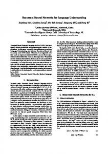
The result was a decent knowledge about a map of the involvement of different brain areas around the sylvian fissure as well as across the frontal cortex in language processing. In most views, language processing was strongly lateralised to the left– dominant hemisphere of the brain with the exception of the sensory input of sounds and the motor output (for summaries, compare [19] or [96], figure 2.1 provides an overview over the brain regions involved in language processing). An additional result was the establishment of early models about the temporal dependencies of the most important regions for language in the brain. For example the influential Geschwind model states that for the task of repeating a word, sounds are first processed in the Primary Auditory Cortex (A1), get further analysed in the Wernicke’s area, get transmitted via Arcuate Fasciculus (ARF) nerve fibres to the Broca’s area, where they get associated, further mapped to sequential articulations in the PreMotor Cortex (PMC), and finally fed to the muscles for the lips, tongue and most importantly the larynx6 via the Primary Motor Cortex (M1) [100].
PMC
STG
M1
A1
pIFG
pSTG
IFG aIFG
pMTG aSTG
dorsal
posterior anterior ventral
STS
aMTG
MTG ITS
Figure 2.1: A map of the human brain (dominant-left hemisphere) with regions involved in language processing. For orientation the map is coloured: the cortex’ temporal lobe in green, frontal lobe in red, parietal lobe in blue, and occipital lobe in light grey as well as cerebellum and medulla in dark grey. Highlighted regions are the Primary Auditory Cortex (A1), Superior Temporal Gyrus (STG) (including anterior and posterior parts), Superior Temporal Sulcus (STS), Middle Temporal Gyrus (MTG) (including anterior and posterior parts), Inferior Temporal Sulcus (ITS), Inferior Frontal Gyrus (IFG) (including anterior and posterior parts), PreMotor Cortex (PMC), and Primary Motor Cortex (M1). 6
The larynx is an organ in the neck that contains the vocal cords and manipulates pitch and volume of sounds.
10
2.1. Three Pillars of Natural Language Research
However, during the last decades neuroscientists started to reject these models as well as the locationists’ view of language processing because of both anatomic and linguistic underspecification [255]. Instead, researchers proposed the view that language processing is distributed widely across the cortex, involves various cognitive processes in parallel, and applies mechanisms for processing language on more than word-level [15, 125, 147, 222, 292]. Two Streams in Language Processing: Re-defining a Fine-grained Map For a number of cognitive functions in the human brain we have obtained substantial knowledge by studying those functions in depth in individuals from the animal kingdom, where the brain architecture as well as the cognitive processes are similar. This is in particular true for the vision system, for which we have a superb understanding about the processing steps and neural architectures from the receptor cells in the retina, which just capture the activation differences of a specific receptive field, up to the neurons in the posterior Inferior Temporal Cortex (ITC), which represent complex 3D-shape information [150]. However, because natural language is unique in humans, we currently have no methods at hand to have a detailed look at the neural processes and wiring in the human brain. For good reason we do not want to conduct invasive studies, where we employ measuring devices in a healthy brain, nor do we have a sufficient number of opportunities to measure on single cell level in cases where a patient needs to undergo a brain surgery for other reasons (for example [211]). Recent advances in Functional Magnetic Resonance Imaging (fMRI)7 as well as the combination with ElectroEncephaloGraphy (EEG) or Near Infrared Spectroscopy (NIRS) allow for detecting brain activity on good spatial or temporal resolutions. Still, all techniques are inherently limited to being precise in one of these dimensions. Nevertheless, during the last decades the initially sparse map of language processing in the brain has been filled with a large number of puzzle pieces, assembling nearly the full cortex being involved in language processing. In particular, based on numerous fMRI and Magnetoencephalography (MEG) studies Hickok and Poeppel hypothesised that two streams are involved in speech processing on word level [124, 125]. Incoming acoustic signals are processed first in the A1, the dorsal surface of the Superior Temporal Gyrus (STG) in both hemispheres, and are analysed on spectro-temporal level. Afterwards, these information get mapped to phonetic representations around the mid-posterior Superior Temporal Sulcus (STS). Both, the A1 and STS, then project to two streams: • A ventral stream maps the phonological representation onto lexical representations in the posterior Middle Temporal Gyrus (MTG) and the posterior Inferior Temporal Sulcus (ITS). This mapping already happens in parallel routes across the brain: On a) a fast route with a signalling rate in gamma range (around 20-50 ms) in both hemispheres and b) a slower route with a rate in theta range (around 150-300 ms) strongly in the right hemisphere. 7
Other methods like Positron Emission Tomography (PET) and Magnetoencephalography (MEG) also had both a tremendous development and important impact on neural data recording.
11
Chapter 2. Approaching Multi-modal Language Acquisition
The authors claim this to be the result of the strong bias of the right hemisphere in general sound (and music) processing as well as the notable part of complex sounds being involved in natural language. From lexical representations (and supposedly low-level syntactic operations) the signals are processed again in parallel further a) in the anterior middle temporal regions (both the MTG and the ITS) in the left hemisphere, where first syntactic and grammatical (combinatory) operations take place, as well as b) to various regions on the whole cortex, where conceptual meanings are mapped. • A dorsal stream maps phonological representations onto a sensorimotor hub in the posterior STG (part of the Wernicke area) that in parallel a) maps the signal to the Inferior Frontal Gyrus (IFG), but also b) integrates multi-modal information from other sensors. Further processing involves the motor integration on the sequence level as well as on the level of segments in the sequence in the IFG as well as in the PMC8 . Based on development (for this thesis more precisely: previous learning) segments of the sequence are either activated as motor chunks or can require incremental motor coding. Overall, the ventral stream captures the recognition of auditory signals like speech in natural language, while the dorsal stream integrates auditory signals with motor actions (see figure 2.2). Similar to the hypothesis on a What path and a visuomotor integration path9 hypothesis in visual processing [193] these streams differentiate between ‘what’ in a semantic sense and the sensorimotor integration in terms of an articulatory representation. In addition the authors suggest connectivity within both streams in feed-forward as well as in feed-back links and the important involvement of a conceptual network that interconnects motor representations with lexical representations across the whole cortex. Both, the lexical representations as well as the associations, involve both hemispheres similarly [25]. dominant -left
nondominant -right
Figure 2.2: Speech processing hypothesis proposed by Hickok and Poeppel (based on [125]). 8
Actually also the neurons in the M1 for tongue and larynx muscles are excited in listening to speech [76]. 9 In traditional views the visuomotor integration path was called the Where path, but according to [125] the function is much more general. For example activation was also measured, if an appropriate motor action was conducted for an object that was no longer visible [234].
12
2.1. Three Pillars of Natural Language Research
For the comprehension of sentences, Friederici et al. suggested that the ventral stream consists of even two structural as well as functional different pathways that also extend with fibre tracts from the temporal gyri and sulci to the prefrontal regions [85, 87, 88]. From both, the phonological word form in the STS and the lexical word form in the MTG the syntactic analyses in the anterior STG obtains phrase structures and word dependencies. The information is further projected via the Uncinate Fasciculus (UNF) tracts to the Frontal OPerculum (FOP)10 and from there to the posterior IFG for higher-level syntactic processing including hierarchical ordering of arguments and phrases. In parallel the semantic processing is proceeded from the anterior MTG, via the Extreme Capsule Fiber System (ECFS) to the anterior regions of the IFG11 . The authors also suggested that the dorsal stream from the posterior IFG to the posterior STG is highly bi-directional and provides feedback from the syntactic analysis to the recognition of new incoming words12 . Figure 2.3 visualises the comprehension hypothesis. dominant -left
nondominant -right
Figure 2.3: Comprehension of sentences according to the hypothesis by Friederici et al. (based on [85, 87, 88]).
For the production of words, Indefrey and Levelt suggested a similar processing across the cortex, but added distinct temporal dependencies and functional roles between different areas (compare figure 2.4) [133]. The first activation occurs in the anterior MTG (around 175 ms after onset of an stimulus in a picture naming task) and is supposed to instantiate a conceptual lexical representation. Afterwards activation is mapped to the MTG for a lemma selection (around 250 ms after onset) and further processed in both, the posterior MTG and the STG, for retrieving the lexical phonological code and its segmentation (around 330 ms). Via ARF fibres the activation is then spread to the IFG, where a sequential order of phonological syllables and words is formed (around 450 ms), and finally to the M1 where 10
Note, among other fibres the UNF may be involved in these connections, but temporarily disabling these connections does not necessarily lead to an impairment in language processing [68]. 11 Although the connecting fibres are close to each other, a distinct functionality was found, e.g. in processing correct sentences compared to processing sentences that are only structurally valid [86]. 12 For example, it was found that a shorter distance between a verb and it’s argument decreases the activity in the phonological working memory [190].
13
Chapter 2. Approaching Multi-modal Language Acquisition dominant -left
nondominant -right
Figure 2.4: Word production hypothesis suggested by Indefrey, Levelt, and Hagoort (based on [111, 133]).
articulatory patterns are triggered (around 600 ms). It is important to note, that parts of this processing pathway have been found in other word production tasks as well: for example for a word reading task, activation starts (after a visual recognition of the word) mostly in the STG, while the reading of pseudo-words mostly starts in the IFG. In recent reflections Hagoort and Levelt also claim an additional activation of the IFG for all processes that involve lemma selection, lexical phonological code retrieval, segmentation and phonetic encoding [111]. In fact, Amunts et al. argued for at least ten distinct subdivisions of the IFG (here again named Broca’s area) in the antero-posterior axis [5], which should imply, according to [219], that at least the same amount of distinct operations is performed in this hub of the brain. Towards Embodied Language Processing In the discussed hypotheses above we have seen that processing of speech activates conceptual networks and that activity in conceptual networks precedes the processes in production. A crucial open question is how precisely concepts are represented. Concerning this important point Barsalou claimed that the representations for semantic entities (“symbols”) are the key and that core representations in cognition, including language processing, are not amodal symbols and data structures [14, 15]. On the contrary the sources of information and representation – that ground cognition – encompass the environment and embodied simulations of perceptions and actions. Evidence was found that both perceptual systems and in particular action simulations are activated in word and sentence processing [102, 103, 254]. In addition, regions that code for entities in perceptions are activated previous to word and sentence production [107, 133]. Pulvermüller defines embodiment as the overall term for the theory that cognitive processes including language processing are semantically grounded in sensation, action and bodily experience [224]. He claims that cognition originates in bodily interactions with the environment. Furthermore, even higher cognition is affecting sensorimotor variables and the brain’s modal system. For language processing he argues that action-perception circuits are a necessary and important part in 14
2.1. Three Pillars of Natural Language Research
semantic processing. This applies to semantic concepts of physical entities in the world, for words on actions that modify entities, and for higher concepts. Examples are: • Words that are shape-related show strong activity in regions for visual shape processing, mostly ventral in the posterior fusiform area (where 2D shape processing takes place), but also in dorsolateral regions (where 3D shape information and relation is processed) and similarly colour-related words have activity also in vision area around the ventral fusiform area [225]. • Words that are related to body parts like arm- or leg-related words show strong activity also in the somatomotor cortex around these spots were motor commands for arm or leg movements are executed [226]. • Words that are rather abstract, like beauty or free, supposedly show activity in higher vision areas in the inferior temporal cortex or the higher bodyaction areas in the prefrontal cortex, both as part of a complex circuit on the cortex [224]. In processing words, these action-perception circuits can be observed in conjunction with a basic spoken word form that activates areas in STG as well as IFG regions (compare figure 2.5). The specific activity within the action-perception circuits for words as well as for phrases is mainly depending on the location of specific perceptual nodes that respond to the actual perception or action of that entity and can be spread across both hemispheres (for an example on the shape-related action-perception circuit see figure 2.6) [223, 227].
(a) spoken
(b) arm
(c) shape
(d) colour
Figure 2.5: Conceptual webs in terms of activity pattern for different word forms according to Pulvermüller and Fadiga. From left to right: basic spoken form, arm-related word, shape-related word, and colour-related word (based on [225]).
In line with these findings Borghi et al. claimed that the sensorimotor system is supposed to be involved during perception, action and language comprehension [30]. In their review and meta-analysis they added that actions as well as words and sentences which are referring to actions are firstly encoded in terms of the overall goal (the overall concept) and then of the relevant effectors. In addition, Pulvermüller et al. suggested that for specific combinations of lexical and semantic information a combination of areas, including auditory, motor, or olfactory cortices, can act as binding sites [223, 224, 229]. 15
Chapter 2. Approaching Multi-modal Language Acquisition dominant -left
nondominant -right
Figure 2.6: Activity pattern (indicative major foci) for a “form” (visual shape) related phrase according to Pulvermüller et al. (based on [223, 227]).
Biology of Language Revisited: Perspective of Distributed Language Processing In summary, the research in speech processing, speech production, and language comprehension vastly revised the view on processing in the brain during the last two decades. The evidence emerged substantiated the idea that language processing is not taking place in the dominant-left-hemisphere only and is not mainly centred in the Broca and Wernicke area. We now have the knowledge that the right hemisphere is strongly involved in all aspects: in analysing sensory input in posterior regions, in comprehending input, and initiating the production of output in frontal regions [28, 53]. Also we have a good understanding that numerous strong interconnections – or fibre bundles – across the brain connect various areas in the brain that are spatially distant [110]. Additionally, in some brain regions, like in the IFG and the Sylvian Parietal-Temporal (SPT), small areas are supposedly working as central hubs for information, mainly interacting with a large number of regions on the cortex [124]. With these data, neuroscientists redraw the map of language on the cortex, although there exists no coherent theory yet. On a more detailed level we can summarise the involvement in language as follows: • A1 and anterior part of the STG – both hemispheres: maps sounds to phonological representations, • STS: phonological network, • Anterior ITS: combinatorial network, • Posterior ITS – both hemispheres: interface to lexical mappings, • SPT, partially overlapped with Wernicke’s area (posterior superior temporal gyrus): interface for multi-modal sensory input, • IFG, also named Broca’s area: acoustic associations and low-level syntax, • PMC: articulations, sequence thoughts, involved in action-perception circuits, • M1: muscular control for speech, involved in action-perception circuits, 16
2.1. Three Pillars of Natural Language Research
• Extrastriate gyrus (V3, V4, V5): shape recognition (mainly in V4) and visual symbol/word recognition, involved in action-perception circuits. With this more fine-grained map neuroscience could provide answers to the initial questions about the “Where” and “When”, but directly opened up two more central questions: • How does a particular cognitive process operate on neural level? • Why are particular neural architectures the ideal solution for the process from a biological perspective? Accounts on spatial processing hierarchies as well as on action-perception circuits and embodied language processing gave us valuable information about connectivity in the brain. In particular, evidence for distinct timescales in both, processing perception as well as producing speech, might indicate an architectural characteristic that may be crucial for language. In addition, the memory traces or cell assemblies in action-perception circuits can contribute information of varying degree in natural language phrases (both will be discussed later in chapter 4.1). However, neuroscience could not provide sufficient data or feasible models on functional details like plasticity and temporal dynamics yet [228]. In a recent reflection Poeppel added that for linguistic operations, higher than the sound to phoneme mappings, models for architecture of the neural circuits are currently “pure speculation” [219]. In particular, for combinatorics and compositions we have neither theory nor model. it is critical that models of the sensorimotor system differ in varying degree from the human one [30]. This might allow understanding which aspects of the humans’ neural and sensorimotor system are critical. Phonological and Lexical Priming Another impact of the neuronal wiring are priming effects in language processing. In general, priming is understood as the activation of related circuits after the initial activation of a specific sound or engram. The result of this priming is a faster processing of expected traces of activity. In more detail, two different forms of priming have been suggested and supported with reasonable evidence for both, processing incoming speech as well as producing speech. On the one hand, a phonological priming takes places in young children (up to 18 months of age) [186]. After a specific incoming sound is perceived, cohorts of engrams (mostly words) are activated (in the mental lexicon) that follow up on the same sound (syllable). For example after the processing of the sounds ca a cohort of known words of candidates like candle, candy, and carrot are activated. For production, Levelt et al. in fact showed that after the phonological code for a lemma is selected, sounds are produced incrementally and in turn prime competing (semantic) forms of the lemma with similar phonology [161]. On the other hand, a semantic-lexical priming can be observed in older children up to adults [159, 180, 267]. In this setting, a primer is not only the previous sound, but the sounds including the lexical meaning of the engrams processed before. 17
Chapter 2. Approaching Multi-modal Language Acquisition
For example, Spivey et al. showed in a hand pointing study, that the reaction in deciding for a scene is faster towards the correct scene after an incoming word describing that scene – in contrast to a distractor – was perceived [267]. Similarly for production Levelt suggested that after selecting and triggering the first lemma for a context, the upcoming lemmas in the mental lexicon are accessed faster in comparison to distractor lemmas [160]. This means that for a language learned with a larger vocabulary the cohort activation shifts to the lexical level as a much stronger influence on the upcoming processing. Although the threshold of the transition between stronger impact of phonological priming to semantic priming is still debated, both are believed to build an important organising principle for the engrams (words) in the developing mental lexicon [172, 180]. Phonological and lexical priming not only effects the efficiency by pruning unlikely sequences but also reinforces the neural circuits that represent an engram or a context.
Introducing the Neural Binding Problem With all the principles discusses so far we have observed that information processing can get influenced and in a sense implement a gradient of entropy in the noisy data of sensory experience. Central and still missing is the problem of how items (or again engrams) are integrated and meaning emerges. This is often called the binding problem, but the formulation varies within the neuroscience domain [139]. Originally Malsburg described this problem as the lack of understanding how encodings of said items within distinct brain circuits are integrated to determine a decision or action [179]. Feldman specifies the neural binding problems over complementary dimensions: activity coordination or temporal synchrony, subjectivity in perception, visual feature-binding, and variable binding [79]. For example, the visual feature binding concerns how spatially distant neurons that code the same feature fuse a meaning. Here, the problem is seen solved by e.g. the theory of synchrony of cell firing. For instance Engel et al. showed that networks of neurons communicate by firing patterns [73, 74]. In particular, it was shown that neurons that both respond to the same visual stimuli (could be vertical orientation) fire in synchrony and that meaning is coded by oscillations in the firing. As second example – central to this thesis – the neural variable binding concerns the relation of items in a temporal sequence that need to be bound into a meaningful concept. Transferring the idea of synchrony to the temporal dimensionality was demonstrated e.g. in the SHRUTI model [256, 257]. Therein the temporal stream is divided in phase cycles, and items within this stream may fire in synchrony with previous items and thus bind roles (or specific role fillers). However, so far neither clinical studies nor simulations to support this concept in variable binding are available [78, 79]. Thus we still need to find an appropriate neural mechanism to acquire roles and concepts in processing natural language sequences. 18
2.1. Three Pillars of Natural Language Research
2.1.3
Top-down in Behavioural Psychology
Behavioural psychology is the scientific field focused on explaining and predicting behaviour. In particular, cognitive psychology and developmental psychology aim at explaining mental processes in humans and how they change over time. For language both disciplines describe processing and acquisition in light of human interaction and observable stimuli as well as effects. Developmental psychology is particularly important, because it studies the socio-cultural principles shaping the language acquisition13 . Central findings are the phases of language development all children undergo consistently14 and the impact the environment as well at the caregiver – or more precisely the language teacher – have. Cognitive psychology studies mental mechanisms and principles in perception and production. Especially findings on the learners body-centric modelling as well as on statistical characteristics of feedback are of particular importance. Children’s Development in Natural Language For language acquisition the first year after birth is most crucial. In contrast to other mammals the human child15 is not born mobile and matured, but develops capabilities and competencies postnatal [145]. The development of linguistic competence occurs in parallel – and highly interwoven – with the cognitive development of other capabilities such as multi-modal perception, attention, motion control, and reasoning, while the brain matures and wires various regions [78, 145]. In this process of individual learning the child undergoes several phases of linguistic comprehension and production competence, ranging from simple phonetic discrimination up to complex narrative skills [106, 145]: • Prenatal: auditory system gets tuned to the mother’s voice and its phonetics (vowels). • 0 – 5 months: perception of sounds, rhythm and prosody; production of reactive sounds and imitation of vowels. • 5 – 9 months: inter-modal perception; canonical babbling, imitation of intonation, and production of vowels. • 9 – 12 months: perception organised toward a phonological structure (map in A1 [231]) and segmentation and comprehension of words; production of first words; also pointing and iconic gestures are used as a pre-lingual method to express desires before the correct vocalisation is acquired. • 12 – 16 months: comprehension with a corpus around 100 to 150 words and simple holo-phrases; production of around 20 to 30 words to name or request objects or actions. 13
Or as discussed above, more precisely enable the acquisition in the first place. Individual variability and underlying factors can be determined reasonably fine-grained [55]. 15 As a convention we use “child” to refer to a language learner of any age ranging over new-born baby, infant, toddler, and preschooler. 14
19
Chapter 2. Approaching Multi-modal Language Acquisition
• 16 – 20 months: establishment of the comprehension of word categories; production of two word combinations and undergoes a vocabulary spurt. • 20 – 24 months: comprehension of word relations and word order; reorganise phonological production. • 24 – 36 months: comprehension of complex sentences and inference of grammatical rules for own production. • 35+ months: start comprehension of metalanguage; syntax and morphology tuned in production. During this development the child is exposed to steady streams of perceptualcognitive information from the environment and its interaction with it. This can include both the perception of physical entities in the environment as well as a stream of spoken natural language for describing it and leads to the association of a sequence of sounds with that entity – a preposition for reference. Smith and Yu showed that infants can indeed deal with an infinite number of possible referents in learning the first words by means of rapidly evaluating the statistical co-occurrences of words and scenes [265]. They revealed in their study that 12 – 14 month old infants can solve the uncertainty16 across several trials with many words and many referents (e.g. objects). The authors claim that the learners actual make use of the complexity of the natural environments in terms of tracking multiple word-referent co-occurrences and their underlying regularities. Psycholinguistics found a number of further critical principles working in language acquisition, including segmentation, body-relationality17 and social cognition [41, 106]. Segmentation: From Sounds to Utterances The principle of segmentation is found very early in children’s development, as the new-borns are believed to instantly learn to segment vocals within the melodies of the mother’s speech [145]. With more clear evidence Saffran et al. found that infants in fact are able to learn language statistically [243, 244]. In their studies they showed that 8-month infants can learn to segment words solely based on the frequency of co-occurring syllables within continuous streams of speech that contained no further information on word boundaries like pauses or other acoustic or prosodic cues. Tenenbaum and Xu suggested that the early word learning follows the Bayesian inference principle [279]. In their study they proposed that correct word-referent mappings can develop fast by formulating and evaluating of hypotheses. For example, a wrong hypothesis formed in a first learning step could be corrected in a second learning step (again in an ambiguous scene) thus providing dis-confirming evidence. As a result this means that children can learn to segment words mostly by the usage. In this way they also learn novel words by exploiting highly familiar adjoining words. 16
Originally referred to as indeterminacy problem in deriving meaning. Smith and Gasser originally named it the embodiment principle [264], but the definition for embodiment as given above is much more specific and central to this thesis. 17
20
2.1. Three Pillars of Natural Language Research
Body-rationality: The Egocentric View on the World As discussed earlier, the human intelligence in general and language competence in particular is strongly driven by the rational integration of the body in the environment. Sixty years ago Piaget suggested that any representations, which children might form, should have developed through sensorimotor level environmental interactions accompanied by goal-directed actions [216]. According to Smith and Gasser the physical world indeed contains rich regularities that constrain the human brain in perceiving and acting [264]. In developmental studies18 they found that knowledge can be realised by the body in a way that relative links to entities in the environment are available. In turn the knowledge can be stored and obtained just by the relation of aspects of the body to the link. For example linking objects to locations (and thus by a specific perception for that relative location) and linking events to the location and thus the object is sufficient to bind objects and predicates. In fact, Smith and Gasser claim that the embodiment is the necessary precondition for building up higher thoughts. Social Cognition: Language Learning Through Interaction As introduced in section 2.1.1 the development of language was only possible by interaction of a child with a developing brain and a teacher that provides digestible amounts of spoken language [280]. Tomasello calls this inter-subjectivity and claims that the human is not only building up thoughts by linking the body to the environment, but also developed an awareness for the body-rational view on the world of others. Humans developed a profound competence to respond to motives and interests behind motions of others including to support expressing them. Hayes and Ahrens found from large data collections of natural conversations between children and their mothers that the mother provides an age-dependent simplification of grammar and focuses on more common words [114]. The word choice is supposedly based on the context of the common conversations and meant to kept lexically undemanding. In particular, Grimm refers to the mother-child interaction as a didactic system accompanying the development phases [106]: • 0 – 12 months, baby talk: exaggerated intonation, long pauses between phrases, and simple words to support prosody and phonology, • 12 – 24 months, scaffolding: joint attention and introduction of specific words to support the vocabulary (e.g. by pointing and active labelling [112]), • 24+ months, motherese: model-language and questionnaires to support grammatical competence. Overall this means that the postnatal development of the processes of thought together with an appropriate interaction of the teacher enables the acquisition of language. 18
Studies included the Baldwin task, in which 24-month-old children name objects correctly, for which they learned the labels under the condition of visual occlusion, but specific location [264].
21
Chapter 2. Approaching Multi-modal Language Acquisition
2.2
Bridging the Gap: Developmental Robotics
In between the aforementioned areas of research, Linguistics, Neuroscience and Behavioural Psychology, a new interdisciplinary field is emerging. Aiming at providing massive data corpora, vast simulations, and roughly realistic robotic re-enactments of mother and child scenarios for learning a language in natural environments, Developmental Robotics (DR) was initiated as the interdisciplinary interface between, but not limited to the three established fields [7, 43, 291]. More specifically Cangelosi and Schlesinger describe Developmental Robotics (DR) as “the interdisciplinary approach to the autonomous design of behavioural and cognitive capabilities in artificial agents (robots) that takes direct inspiration from the developmental principles and mechanisms observed in the natural cognitive systems of children.” [41, p. 4] The general approach in DR is to study integration and complexity opposed to the conventional approach used in the established fields to divide a phenomenon into the smallest and simplest entities and study these entities profoundly in hope of shedding light on the bigger picture. For doing so, the core methodology is to construct computational models and robotic architectures of language representation, language processing and language learning to test and combine linguistic hypotheses that are difficult to get verified by the other fields alone because of the inherent limitations of their methods and most importantly the complexity of language in whole: • Where behavioural studies can only hardly dissect the child’s reasoning and cognitive processing, traces of computational results can be analysed. • What neuroscience measurements can obtain in 40 years, computer simulation can generate in two hours [108]. • When theoretical accounts get criticised for difficult assumptions and constraints, which may be hard to maintain in noisy and cluttered real situations, robotic interactions can be tested in real environments. The biggest strength of the DR approach is that studying in real world scenarios a) inherently forces to avoid oversimplifications and thereby reduce underspecification as well as b) fosters to include the uncertainty that human children have to deal with, in the real world.
2.2.1
Adopted Principles of Language Acquisition
In bridging the gap, DR heavily builds on top of findings of and relies on constant input from the other fields (compare figure 2.7). DR borrows insights of child psychology research, in particular developmental and cognition studies from behaviour psychology. To neuroscience DR ows insights provided by new imaging technology in brain science and theoretical accounts on internal mechanisms. From linguistics DR adopts theories on language construction and its origins. 22
2.2. Bridging the Gap: Developmental Robotics
Developmental Studies
Behavioural Psychology Cognition
Language Evolution Etymology
HumanRobot Interaction
Developmental Robotics
Derive Measure Observe Principles Activity Behaviour
Derive Hypotheses
Develop Model
Linguistics Computational Linguistics
Simulations
Systems Neuroscience
Test Model on Robotic Platform
Neuroscience Imaging Studies
(a) Bridging natural and social sciences.
Compare Principles, Activity, Behaviour
(b) Methodology.
Figure 2.7: Developmental Robotics approach: adopting principles found in language acquisition from natural and social sciences. Robots or agents are constructed based on theories from linguistics, behavioural psychology, and neuroscience and are tested through interactions with an environment.
For example in language acquisition studies, the developing robot could borrow an inherent predisposition for reference and employ algorithms for preprocessing (segmentation) as well as for rational robot-centric representations. Robotic learners often inherit a social cognition paradigm to utilise some kind of shared attention or cooperation mechanism [280]. According to Cangelosi and Schlesinger, developmental robotics often relies among others things on basic principles of cognition such as similarity (a label for a entity is generalised to similar entities), conventionality (individuals in a close community use the same word for certain meanings), and mutual exclusivity (noun labels refer to exclusive object categories, and categories have only one label) [41, 51]. Depending on the level of looking at language acquisition from first sounds to complex linguistic constructions, other principles or biases in development from the classical fields are included or subject to examination.
2.2.2
The Case of Neurobotics
Neurobotics is a special case within developmental robotics, where a robotic controller is designed bottom-up from a neural system. This robot is supposed to demonstrate the effect of the neural architecture for input data in particular or the reaction of the neural system in a specific natural task in general. Opposed to 23
Chapter 2. Approaching Multi-modal Language Acquisition
mainly developmental-psychological driven approaches in developmental robotics, where the system is designed top-down with the aim of understanding what caused a specific behaviour, the neurological robotics (for brevity often written as neurobotics) seeks to understand which effects emerge from a specific neural structure. Research in neurobotics adds the noise and uncertainty of real world experiments to neurosimulation.
2.2.3
Contribution of Related Studies in Developmental Robotics
Most studies on language processing, which adopted the DR approach, focused on the development of robotic agents that are grounded in real world scenarios. By means of inspiration from neural mechanisms, this particular approach allows to study the characteristics of language learning in computational models to solve the grounding problem by neural binding. For example, one of the first of such models addressed the fusion of language and multi-modal perception and aimed at bridging the gap between formal linguistics and bio-inspired systems [239]. Models with increasing complexity followed, addressing the grounding of proto-words (‘symbols’) in object manipulation and robot movement [39, 292], the grounding of a symbolic representation in learned actions that in turn can be generated with affordances, goals, and policies [203], the grounding of higher-order symbols in action primitives and in sensorimotor experience [270], and the grounding of words in both object-directed actions and visual object sensations [77]. As an exemplary bridging contribution, Wermter et al. described two models for neural grounding of language processing in actions, embedded in a robotic platform [292]. The authors developed single-layer and hierarchical architectures which consist of a Helmholtz machine-based associator network with language, high-level vision and motor action inputs. The robots, on which these architectures have been implemented, were supposed to learn and perform on command three behaviours: go, pick, and lift. The single-layer architecture relied on a competitive winner-take-all coding scheme, while the hierarchical architecture combined a sparse and distributed coding scheme on the lower layer and a winner-takes-all coding on the top layer. In both models, the authors followed the mirror neuron system concept, which was suggested for the human and primate F5 brain region. As a result, their models recreated the neuroscience evidence on word representation (compare section 2.1.2 and [226]) and contributed some insights on the organisation and activation of sensorimotor schemata from a computational modelling perspective. Hence, the particular contributions are predictions on the mechanisms behind the observations made in neuroscience, based on embedding and testing the model in the real world. The related work on grounding, binding, and multi-modal integration is of particular interest for this thesis. Further specific studies, however, will be discussed in detail in the chapters 5 and 6. 24
2.3. Objective and Research Question
2.3
Objective and Research Question
With the findings and general state of the art discussed, we now can refine the goal of this thesis. The principles and hypotheses that we learned from recent research studies in neuroscience, behavioural psychology, and linguistics should influence both, the brain-inspired architecture as well as the environment and mechanisms of the language acquisition. With the methods from computer science, the objective is to develop and study a neural architecture based on the human brain for processing sequences of sounds over time, but also to include the processing of perception from the environment. This architecture is supposed to learn natural language and also to generalise. Based on the developed architecture, studies will include observing how the language is represented internally and which factors lead to a successful acquisition of the language. Specifically, the key research questions for this thesis are: • How can natural language emerge from a neural architecture that comprises hierarchical abstraction and timescales in information processing? • How can an embodied but compositional representation self-organise solely by processing sequences of natural language and reference candidates in terms of sensory context? • How can a multi-modal embodied context foster developing a language competence? • How can similar representations for concepts emerge in speech comprehension as well as production? To support the acquisition of language on a level beyond holo-phrases, both body-relative and by means of social interaction, the research also must include technical means to embed a physical (robotic) learning agent into a real environment and to actually learn from language examples. This includes that the learning robotic agent is able to pick up language from a mother-like teacher and to ground the acoustic information in visual or both, visual as well as sensorimotor stimuli. Additionally, the neural architecture must be enabled to self-organise upon the data. Those needs lead to two further research questions: • How can we enable a robot to learn from speech in human-robot interaction as well as from uni- or multi-modal sensory input? • How can we train a cortical recurrent deep neural architecture with large sequences of natural language? The focus for the research questions lays in fundamental research, which means the emphasis is stronger for understanding the mechanisms in the brain and not so strong for the utilisation in applications. 25
Chapter 2. Approaching Multi-modal Language Acquisition
2.4
Impact and Timeliness
Although research about language acquisition has a long history, we still have no clear idea of how humans develop language competence. With the new developments in imaging methods in neuroscience, we now have a much better means to investigate how language emerges in the brain. Nevertheless, we are currently looking at the what, where, and when, but cannot measure how. With the proposed objectives, this thesis aims at contributing to this specific gap. Using the approach of developmental robotics, the important contribution is to assemble the missing pieces in the puzzle to understand how language is represented and acquired given the facilitating or hindering characteristics of the human brain’s structure. Succeeding at this point could provide new research questions for fundamental research in neuroscience and developmental psychology towards connectivity characteristics or learning mechanisms. Important for research in neuroscience could be an insight in dynamics and self-organisation in neural models. First of all, a developmental model could test how architectural characteristics influence, whether a language competence can be acquired. Accordingly, an architecture can adopt spatial but also temporal hierarchical dependencies on certain processing stages (sounds, lexical access, concepts) from recent neuroscientific theories (see section 2.1.2). In turn the model can report specific architectural constraints and predict certain activity patterns that can define the focus of future imaging studies. Secondly, another model could test embodiment integrated in language on several levels and study how the architectural characteristics foster the language acquisition. Such an architecture might reproduce multi-modal integration and provide information about how distributed conceptual representations form under temporal dynamic conditions (compare section 2.1.2). Future research endeavours thus can measure the processing of information in the brain in language tasks for different conditions of multi-modal input. For the research in developmental psychology, the developmental robotics models are able to inform about the importance of certain multi-sensory perception in language learning to develop new strategies for supporting language learning of infants. Additionally, results from the models can motivate further studies on how the learning of holo-phrases and short utterances is organised in humans (compare section 2.1.3). Finally, for the debate in linguistics on generativism versus constructivism, the models can provide support for either of the positions (compare section 2.1.1). For application however, this could open up and set the basis for a completely new interpretation of language processing in human-like machines that are supposed to support humans in daily life. On the one hand, speech recognising architectures that operate on the human-level concept of language could be considered opposed to relying on the current pipeline approach based on artificial modules for models and hypothesis search. On the other hand, machines could be developed that would be able to learn language with a human-like body-rationality and thus could understand new tasks in real, but unknown environments. Such a robot could exchange the right information, understand situations to react with proper actions, or even collaborate in tasks with the human. 26
2.4. Impact and Timeliness
The need for the latter is already emerging: Robotic companions’ hardware can be produced for reasonable prices with reasonable capabilities, while the need for companions in daily life, in particular in health care, is getting pressing. Just recently, the Bundesministerium für Bildung und Forschung (BMBF) (ministry of science and development of the German government) emphasised this goal by announcing the research programme “Technik zum Menschen bringen” (“taking technology to the people” [38]) with the focus on Human-Technology Interaction (HTI) as a central innovation strategy for Germany. Key research questions are how to integrate robots safely in the daily environment, how to develop reliable cooperation partners, and how to secure trustfully interaction. The iconic image for this program is a human communicating with a humanoid robot as depicted in figure 2.8a. At the same time, the International Federation of Robotics (IFR) already plans ahead and forecasts a tremendous increase of service robots getting employed in daily life [134]. As shown in figure 2.8b, predictions quantify an increase of household robots from 3.3 million in 2014 to 25.9 million in 2015–2018 and of entertainment and leisure robots from 1.3 million in 2014 to 9.0 million in 2015–2018. Overall, research in the area of DR to develop cognitive systems in general and architecture for language acquisition in particular is very timely and of substantial relevance for both, fundamental research and application. A computational model can boost to shape theories on language acquisition and to build robot prototypes capable of human-like natural communication. 30
Units sales (in million)
25
2013 2014 2015−18*
20 15 10 5 0
Household Entertainment (b) Service robots forecast by IRF.
(a) HTI view by the BMBF [38].
Figure 2.8: Timeliness of research on language acquisition for human-robot interaction: current view on Human-Technology Interaction (HTI) by the Bundesministerium für Bildung und Forschung (BMBF) (based on [38]), and a recent trend of the need for service robots in households as well as for entertainment and leisure by the International Federation of Robotics (IFR) (* indicates a forecast; based on [134]).
27
Chapter 2. Approaching Multi-modal Language Acquisition
2.5
Methods and Demarcations of this Thesis
The central method to approach the research questions are neurobotic experiments with data drawn from real-world human-robot and robot-environment interactions. For the robot interaction, methods have been developed and improved for natural speech recognition as well as object perception and are described in more detail in chapter 3. For the robot’s neural architecture, neural network properties and training methods have been examined as well as improved and are described in chapter 4. Respective details and metrics for evaluation are presented at appropriate position. To reach the goal of this thesis, some aspects need to be excluded that seem related to the posed research questions. In some scientific views communication with body postures or gestures is strongly related to language acquisition. On the one hand, there is a substantial body of work showing that a) grasping gestures are used to indicate a desired object in a very early development stage (5–12 months) and b) pointing gestures are usually strongly connected with achieving joint attention [41]. On the other hand, many researchers in language acquisition see gestures as an early and simple substitute of vocalising needs, before the phonetic competence has been acquired [78]. Beyond that point, gestures are often seen as a social artefact and are used very differently among cultures. For this reason and due to the own complexity of this field, nonverbal forms of expressing communication are excluded from this thesis. Since for this thesis a central aim is to avoid less plausible assumptions and technological short-cuts, the results may seem limited when it comes to directly applying the suggested architectures in service robots for language learning from scratch. However, the studied characteristics supposedly will be an important stepping stone for developing such a prototype in future endeavours, as suggested in the recently approved TRR project19 . In addition, even with developmental robotics we are not limitless when it comes to mimicking human experience in the real world. For this thesis we need to acknowledge that available robotic platforms, compared to children, still show discrepancies in sensory and actuator capabilities. Moreover, the computational capabilities are limited in terms of to learning in neural architectures. As a consequence, real world experiments need a reasonable simplification. Nevertheless, it will be argued why specific setups are feasible and substantial to draw the respective conclusions. Finally, this thesis aims at in-depth analysis of architectures in question and may seem come short for broader comparison with alternative methods (in particular in terms of network architecture and training methods) that are based on difficult assumptions, but may be advantageous regarding efficiency. To reduce these concerns, we will discuss in detail at appropriate position why a comparison seems not feasible and why different methods still have their place.
19
Collaborative Research Centre TRR169, funded by the DFG [http://dfg.de].
28
Chapter 3 Developing Foundations for Natural Human-Robot Interaction This chapter is focused on describing several methods that have been adapted or developed to allow for studying neural architectures in a neurobotic setup. For this, we will discuss briefly the developmental robotics approach in conjunction with the neurobotics approach and review the state of current robotic opportunities to study systemic functionality and behaviour in the real word. In further reports it will be described in detail, how speech recognition and visual object recognition methods can be applied and made plausible for Human-Robot Interaction (HRI) in language acquisition.
3.1
About Developmental Robotics and the Real World Factor
In chapter 2, we discussed the methodology of Developmental Robotics (DR) in general and learned that this approach is fundamentally different from conventional research of phenomena in language acquisition. The crucial shift in perspective is that we are interested in providing an informed controlling architecture, which is able to develop by interaction with its environment instead of programming a controlling architecture with all necessary knowledge and capabilities. To fulfil the condition of having the environment driving the robot’s development, it is quite crucial that we enable the robot to access the environment as unconstrained and realistic as possible. In general, when it comes to studying human cognitive functions, current DR research relies on humanoid robots with human-like senses [22, 41]. A humanoid robot most centrally has an anthropomorphic body-plan on a child-size scale. Central to this body is a head and torso structure that allows for naturally addressing the robotic learner in communication and joint attention. Senses often include cameras for vision, multiple microphones for speech and sound, arms for nonverbal communication as well as feasible in29
Chapter 3. Developing Foundations for Natural Human-Robot Interaction
teraction with the environment, and multiple sensors in the body for distance or pressure measurements. Bi-pedal movement as well as human-like sensitive skin can be added for certain research questions, but it is currently difficult to achieve budget- and labour-wise [7, 41]. For language acquisition in particular the robot learner needs to be able to sense environmental properties and perceive auditory information on a low level and close to real time with controlled or avoided distortions of the realistic noise [291]. In studies on grounding for example, the DR platform must provide feasible resolution in space and time in auditory input and other senses with minimal overhead to supply a plausible link between the inputs.
3.1.1
Neurological Robotics and Uncertainty
The requirements for our neurobotic1 language learner thus are a preprocessing and encoding of information towards neural activity in the brain’s primary sensory cortices [291]. For auditory information this means that with any cortical model we should not assume more than a structured map of phonemes getting activated sparsely and perhaps in parallel when time passes (compare section 2.1.2). Regarding visual information, we need to make simple visual features for different properties of entities in the environment available. For example, a plausible preprocessing should make simple and unlabelled form (shape) and texture (colour features) features available for objects in the field of view in parallel to auditory information (compare section 2.1.2). Moreover for motor feedback – or more specifically sensorimotor information – a robotic platform must provide to generate information of body states while physically interacting with the objects and to make this information available in terms of a somatosensory map. Children, whose development is driven by the integration of the body in the environment, are inherently exposed to the environments regularities, but also to its uncertainty and imprecision (compare chapter 2.1.3). For example speech processing is immanently uncertain due to referential ambiguities and sensory noise [10, 265]. When taking the noisy characteristics of the real world into account, the filters of the platform’s sensory devices must be fully controllable to acquire data including natural sensory degrading by environmental auditory noise and changing light condition.
3.1.2
Platforms for Developmental Robotics
To enable this research approach, it is a central prerequisite to employ a robotic system that is – in most or in the focused aspects – capable to perceive, act, or interact in its environment as a human does, from a technical perspective [41]. Ideally, this means that the robot (the developing artificial agent) has both, the physical conditions and the interfaces for the mental condition of a human for the respective desired developmental state. 1
For definition see chapter 2.2.
30
3.1. About Developmental Robotics and the Real World Factor
Admittedly, approaching this ideal includes a large number of substantial technical challenges. To present some examples, a robot supposedly visually experiencing a real environment would perhaps need a stereoscopic vision with high resolution and speed; a robot manipulating objects would need hands with fine-grained fingers and pressure sensors in the finger tips; and a robot acquiring language may need to comprehend and produce speech. Integrating these exemplary capabilities into a bi-pedal moving robot includes the handling of large quantities of additional noise and uncertainty due to shaking (in vision), high dimensionality (in body action), or ego-noise (in speech). A robotic platform that could handle these demands would be extremely hard to build (and thus expensive) and excessively laborious to maintain. However, a number of international research teams and companies are making a constant effort to develop robots that fulfil those requirements in varying quality. Central for DR is the Cognitive Universal Body (iCub) robot, which is the result of an international research consortium funded by the European Union with the aim of developing a child-like robot that could be the central and commonly used platform among the research community [189]. The robot provides human-like body proportions, movable stereo-vision cameras and (in parts) a soft-sensitive skin. However, since the development is focused on manipulation and mobility research, which makes the robot particularly precise in hands, head, and torso, the amount and positions of complicated motors make the robot repair intensive and exceptionally expensive. Other significant platforms are the Advanced Step in Innovative Mobility (ASIMO) robot by Honda2 , which is a teen-size humanoid robot, with focuses on walking or other tasks in the setting of acting with and like humans, and the Child-robot with Biomimetic abilities (CB2 ) robot as the result of the Asada lab, which excels in bio-mimicking the whole body, particularly the skin [8, 192]. Other robots that partially fulfil the requirements are robots developed for RoboCup or RoboCup@home [271]. Opposed to developmental robotic research, here the aim is solve simple realistic tasks from human daily life and within the complex human environment with every technical means necessary. Although robotic and software approaches are often inspired by nature and by humans in general, the focus is to make use and push forward existing technologies. The robots from small labs often differ vastly. They are specialised for specified tasks that change annually, but are generally more affordable. As one example the Nimble Robot Open Platform (NimbRo-Op)3 abstracts a human-like body shape in a light, but sturdy case and includes a basic wide-angle camera, replaceable Robotis Dynamixel4 motors in all joints, and current computation capabilities on-board for autonomous behaviour. 2
The company-driven robot and developed frameworks are limited in accessibility. The NimbRo-Op is the product of long-term research at the Universität Bonn related to the DFG project Lernende Humanoide Roboter (BE 2556/2 2004-2012) [253]. 4 Dynamixel motors are cheap servo motors that include potentiometer to measure the motor’s state developed by [https://robotis.com]. 3
31
Chapter 3. Developing Foundations for Natural Human-Robot Interaction
3.1.3
The NAO Humanoid Robot
In between these examples exists the NAO humanoid robot (NAO) [104]. On the one hand, its general characteristic is its humanoid shape with proportions inspired by the human child: the height is about 58 cm, movements are based on bi-pedal walking, environment perception is realised by microphones and cameras in the head as well as pressure sensors in the feet, and the palm of the hand. On the other hand, technical short-cuts have been done in terms of cameras are centred in the head (no stereo vision), body stabilisation is realised with two gyroscopes and an accelerometer in the chest, and the capabilities of the hand are reduced to a tendonbased gripping. With this design the NAO is not ideal for studying the human development in whole, but feasible for investigating a number of specific and fairly constraint cognitive functions and their effect in a medium-range environment. Many modules for control are available and easy interfaced, for example vocalising speech (text-to-speech) or keeping track of sensory perception, particularly somatosensory feedback (hall effect sensors in the motors). Moreover, the platform is overall physically quite robust and precise, thus allowing to reproduce certain actions or behaviour without much calibration. Figure 3.1 shows the NAO robot (a) with a focus on physical characteristics, used for this thesis (b). The NAO is the ideal choice, because auditory, visual, and sensorimotor sensation and movement action capabilities are available with a reasonable abstraction, allowing to adapt and to develop preprocessing methods with reasonable demand, while the robot is overall robust, reliable, and affordable.
(a) The NAO robot.
(b) NAO’s arm and head characteristics.
Figure 3.1: The NAO humanoid robot provides inter alia 5 Degrees Of Freedom (DOFs) in the arm (hand excluded), 2 DOFs in the head, a VGA camera and 58 dBA microphones.
32
3.2. Natural Speech Recognition
3.2
Natural Speech Recognition
For interacting with a learning robotic agent via natural language, it is desirable to use a natural speech input. Natural in this strict sense means without constraints on correct linguistic structure and form. The most important reasons are to teach a robotic learner from a mother’s perspective and to be able to describe arising scenes with appropriate utterances rapidly. For example in the scaffolding and motherese phases mothers would also use single words or holo-phrases5 . However, with the current state of development in Automated Speech Recognition (ASR) an acceptable recognition rate can be achieved only if the system has been adapted to a user or a specific domain and if the system works under low-noise conditions [165, 246]. This is in particular problematic in the language teaching scenario that is related to Human-Robot Interaction (HRI) or Ambient Intelligence Environments (AmIE), where a-priori adaptation for particular speaker is not desired, the usage of close-range microphones like in a headset or cellphone are inconvenient, and robust methods for far-distant microphones are needed [144, 206]. A microphone built into the robot or placed on the ceiling, a wall, or a table would allow for free movement, but would also reduce the quality of speech signals substantially, because of larger distances to the person and therefore more background noise. The central example related to this thesis is the NAO robot, which is equipped with low quality microphones and would be more than one meter distant to a human in interaction. For these particular high-noise conditions most ASR systems usually cannot handle the low Signal to Noise Ratio (SNR) well and result in too low probabilities for the correct chain of phonemes, thus are more likely to determine a false positive utterance. When aiming at natural speech, like in our holo-phrase example, language models inherently offer limited prediction. This is the case for both, open-source systems like Sphinx that offer many options for adaptations and adjustments as well as closed-source system like Google Voice Search (GVS) that operate on much better data and high computational capabilities and inherently offer very good acoustic models, but no options for adjustments [249, 285]. For approaching the research goals of this thesis – employing the DR approach – it therefore is a technical necessity to further improve the available ASR systems with respect to reducing word-error and sentence-error rates to acceptable levels. In the following, we will discuss two approaches that have been developed in conjunction with the main focus this research project. In the first approach, the idea is to combine a domain-specific language model (Tri-Gram) with a domain-specific grammar-based decoder in an open-source ASR. In the second approach, the suggestion is to also make use of the acoustic models from a closed-source system and post-process these results further with domain-specific knowledge. 5
Compare chapter 2.1.3.
33
Chapter 3. Developing Foundations for Natural Human-Robot Interaction
3.2.1
Speech Recognition Background in Short
Before we can dive into the details of the proposed improvements, we first need to look at some relevant fundamentals of a statistical speech recognition system and the architecture of a common single-pass decoder [246]. The input of a speech recogniser is a complex series of changes in air pressure, which through sampling and quantisation can be digitalised to a pulse-code-modulated audio stream. From an audio stream the features or the characteristics of specific phonemes can be extracted. A statistical speech recogniser, which uses a Hidden Markov Model (HMM), can determine the likelihoods of those acoustic observations. With a statistical language model or a finite grammar, a search space can be constructed, which consists of HMMs determined by the acoustic model. Both, language model and grammar are based on a dictionary, defining which sequence of phonemes constitutes which words. Language models are trained statistically, based on the measured frequency of a word preceding another word. With so-called N -Grams, dependencies between a word and the (N − 1) preceding words can be determined. Since N -Grams of higher order need substantially more training data Bi-Grams or Tri-Grams are often used in current open-source ASR systems. A grammar, in contrast, defines a state automaton of predefined transitions between words, including the transition probabilities. During the processing of an utterance, a statistical speech recogniser searches the generated graph for the best fitting hypothesis. In every time frame, the possible hypotheses are scored. With a best-first search, or a suitable search algorithm like the Viterbi Algorithm, hypotheses with low scores are pruned. The result usually is the highest scored hypothesis or a limited list of nh best hypotheses. Both introduced methods, the Tri-Gram decoder as well as the Finite State Grammar (FSG) based decoder, have specific advantages and limitations. • With an N -Gram decoder, an ASR system is more flexible and can get decent results, if the quality of the audio signal is high and the data set for training the language model is sufficiently large. However, since Tri-Grams mainly take the last two most probable words into account, they can deal with long-range dependencies only indirectly. Therefore, even if the word accuracy is reasonably high, the sentence accuracy as a cumulative product is fairly moderate [246]. Larger N -Grams are often not possible due to the need for vast data collections and computational capacities. • An FSG decoder can be very strict, allowing valid sentences without fillers only. Unfortunately, such an FSG tries to map the recognised utterances to valid sentences only. Even if the speaker is just putting words together at random, the decoder will produce a valid sentence and therefore – very often – a false positive. In general, these methods offer a trade-off between low accuracy and specifying the domain. Another common trade-off with respect to accuracy is to also train the acoustic model for a limited set of speakers, thus degrading the speech recognition results for all others. 34
3.2. Natural Speech Recognition
3.2.2
Combining Language Model and Grammar-based Decoder
Since the N -Gram language model approach is unlikely to produce correct results on sentence level and the FSG can produce large numbers of false positives, we can combine the FSG with the classical N -Gram decoder to reject unlikely results. Such a multi-pass decoder could be applied to prone-to-noisy speech input devices such as a ceiling boundary microphone or microphones, installed in a robot. Various approaches for combining FSG and N -Grams decoding processes have been proposed. In particular, for spotting key-phrases in longer sentences, Lin et al. employed N -Gram decoding to cover surrounding phrases of a sentences of interest and FSG decoding, if a start word of the grammar was found by the N -Gram decoder [168]. Levit et al. used an FSG decoder as a fast and efficient baseline recogniser, capable of recognising only a limited number of utterances and a second decoder for augmenting the first decoder by testing for utterances with a similar meaning [163]. Doostdar et al. proposed an approach where an FSG and a N -Gram decoder processed speech data independently based on a common acoustic model, but they did not test for any non-headset conditions [64]. In contrast, Sasaki et al. investigated the usability of a command recognition system using a ceiling microphone array by detecting and separating a sound source and used the input of the ideal microphone for a conventional speech recogniser [248]. However, these approaches tested a very specially optimised decoder set-up for a particularly small-scale problem, they did not test in non-headset conditions, or they avoided the noise conditions mainly by additional microphones. To address problem with regard to the DR approach, a speech recognition approach of combining a language model and grammar-based decoder in a home environment will be presented to address the research question of the effect of the novel multipass decoder in the far-field. We will evaluate the usability in HRI and discuss the conducted investigation of the effect of different microphones, including the microphones of the NAO humanoid robot and a boundary microphone, placed at the ceiling, compared to a standard headset. Multi-Pass Decoder The core idea of the multi-pass decoder is to actually elevate the drawbacks of both conventional decoders on the utterance (or sentence) level. Firstly, the Tri-Gram decoder is used – which is able to back-off to Bi-Grams or Uni-Grams – to produce a reasonably large list of best hypotheses. Even if the best hypothesis of the Tri-Gram decoder is not appropriate, there is a good chance that one of the similar sentences are. Secondly, the FSG decoder is used to produce the most likely hypothesis, even if an out-of-domain utterance is recognise with a valid result. In the next step, the list of nh -best hypotheses of the Tri-Gram decoder is compared with the best hypothesis of the FSG decoder. If a match is found, this sentence can be accepted, otherwise it will be rejected. Figure 3.2 illustrates the HMM-based ASR system using the multi-pass decoder. 35
Chapter 3. Developing Foundations for Natural Human-Robot Interaction
Figure 3.2: General architecture of a multi-pass decoder.
Speech Recogniser and its Adaptation For testing this approach, we can use the ASR framework Pocketsphinx, because it is open source and has been ported and optimised for hand-held devices [131]. In comparison to other promising systems [158, 241], it provides the advantage of being an effective research tool on the one hand and being applicable to devices and robots with moderate computing power on the other hand. Pocketsphinx can be used with a speaker-independent acoustic model ‘HUB4’ based on English broadcast news, but it allows plugging in other acoustic models as well. Since it is our aim to keep the system speaker-independent, it was decided for the test, to limit the vocabulary and to reduce the format of a sentence to a simpler situated grammar or command grammar, as it can be useful in HRI. Devices and robots in our AmIE are supposed to be used for a specific set of tasks, while the scenario can have different interacting humans. The acoustic-model HUB4 was trained with a very large set of data (140 hours) including different English speakers [81]. With a vocabulary and a grammar for the respective domain or scenario, an appropriate FSG automaton can be generated on the one hand and a domain-specific language model can be trained on the other hand. For the training of the language model, the complete set of possible sentences is usually used, which can be produced from a designed grammar by tools offered for Pocketsphinx. In summary, Pocketsphinx can be adapted easily to any scenario, allowing employing various decoders. 36
3.2. Natural Speech Recognition
Testing Scenario and Scripted Corpus Collection The scenario to test the multi-pass decoder was an ambient intelligent home environment, where a human is supposed to instruct, inform or question a robotic platform or intelligent device. This scenario allows to test the ASR under realistic teacher-learner conditions and to relate the approach to other scenarios of humanoid robots in home environments with strong noise conditions and the need for interaction via natural language [197, 291]. In particular, EU research projects like KSERA aimed to develop a social assistive robot, which supports elderly people [220]. The available AmIE is a lab room of 7x4 meters, which is furnished like a standard home without specific equipment to reduce noise or echoes, and is equipped with particular technical devices like a ceiling boundary microphone and a NAO H25 humanoid robot. A human user is supposed to interact with the environment and the NAO robot and therefore should be able to communicate in spoken language (location of the speaker is at a distance of 2.0 meter to the ceiling microphone as well as to the NAO robot). The scenario is presented in detail in figure 3.3.
Speaker
Figure 3.3: Scripted corpus recording: Speech is recorded in parallel by a headset, a ceiling microphone and the four microphones in the head of the NAO robot.
37
Chapter 3. Developing Foundations for Natural Human-Robot Interaction
For the corpus, a grammar for prototypical robot commands over a reduced vocabulary of 100 words was designed6 . The grammar allows for short answers like ‘yes’ or ‘incorrect’, for more complex descriptions of the environment like ‘nao banana has colour yellow’ as well as according questions like ‘nao where is phone’. In general the aim was to allow for generating a corpus that includes in all of these categories a large number of permutations. This is in particular interesting, when the corpus is utilised to test for generalisation and to systematically compare different devices or decoder7 . The set of data to test the approach was collected under natural conditions within our AmIE. Different nonnative English mixed male and female test subjects were asked to read a random sentence, produced from our grammar. All sentences were recorded in parallel with a headset, a ceiling microphone and the NAO robot in a 16-bit format and a sample rate of 48,000 Hz. In summary, 592 recorded sentences were collected each, which led to 1,776 audio files. For the remainder of this thesis we will refer to this data collection as Scripted corpus. Evaluation Result Summary The multi-pass decoder was evaluated comprehensively with focus on the environmental conditions. In particular the question was pursued, how the decoder performs under the open-space conditions of distant microphones with regard to false positives. The specified empirical evaluation method as well as detailed results can be found in appendix D.2. In summary, we can observe that using a multi-pass decoder reduces the number of produced false positives significantly. For low-noise headsets as well as for boundary microphones and inexpensive microphones installed on a mobile robot, reducing the false positives to a large degree does not lead to a substantial reduction of true positives. The overall recognition rates with the NAO were insufficient, while the ceiling microphone worked with a reasonable rate using the multi-pass decoder. An important difficulty in relying on the NAO microphones is the inherent low SNR due to the limited technical property and the strong ego noise, which is induced by the fan in the head of the NAO. The signal offers weak features on the important frequency components for speech, even for applying either the build in noise reduction or the noise filters in Pocketsphinx. A good value for the number of best hypotheses nh depends on the hypotheses space and the utilised microphone, but using nh = 10 is sufficient for our AmIE scenario. Larger values for nh are likely to lead to better results, if the expected quality is moderate and the vocabulary as well as the number of possible sentences are high. Smaller values for nh are beneficial, if the primary aim is to maximally reduce false positives. In fact, setting nh = 1 would mean to accept a hypothesis only, if it was found by both decoder, the Tri-Gram and the FSG, as the best result. Nevertheless the multi-pass decoder is not particularly sensitive to this parameter. 6 7
The full grammar and dictionary is given in appendix D.1. A further use case will be given for another approach within this section.
38
3.2. Natural Speech Recognition
3.2.3
Cloud-based Models and Domain-specific Decoders
For open-source ASR frameworks, the observation was that even with combining multiple decoders an acceptable performance is hard to achieve under noisy conditions. A central limitation for systems is to use an acoustic model that either was prepared for general purpose based on the usually limited datasets available for science or trained on individual data. For example, as of today the 1993 acousticphonetic continuous speech corpus Timit is still used as a notable data set for both, building acoustic models as well as benchmarking ASR systems [94]. In contrast, large corporations like Google, Apple, or Microsoft are able to offer very good and easily retrievable cloud-based ASR services, because they can collect and access vast amounts of data and also process recognition steps on powerful servers [249]. As a consequence, the used acoustic models are excellent and get improved constantly. One particular option is the GVS developed by Google Inc. that works as a distributed speech recognition system. While Voice Activity Detection (VAD) and feature extraction may be performed on the client (depending on the client’s capabilities), the computationally expensive decoding step of speech recognition is performed on Google’s servers, which then returns a list of hypotheses back to the client. The system employs acoustic models derived from GOOG-4118 , but it has been supposedly improved with Timit data and additional data collected in the Search by Voice framework. However, given this origin, a disadvantage of Search by Voice is the language model, which is optimized for web searches. In addition, there is no public interface to change GVS to a custom domain-dependent vocabulary, grammar, or statistical language model. Therefore, the benefit of good acoustic models cannot be exploited well in domain-specific projects [195]. For example, false positives, in particular out-of-vocabulary errors for custom-made natural language understanding components, may be higher with such generic services than with the less reliable open-source speech recognition solutions. To address this gap, we can combine the output from GVS with the domainspecified sub-language of a particular scenario by using a simple post-processing technique based on phonetic similarity. In particular, the result string from the GVS service can be transformed back to a sequence of phonemes which can then get re-scored and aligned to a language model. We can consider phonemes to be the appropriate level of detail that (a) can still be recovered from ASR result strings, and (b) remains relatively stable to different ASR errors that are caused by inadequate language modelling. This method can be realised e.g. with Sphinx-4 and hence works with various kinds of language specifications such as language models, grammars, or blends of both kinds [285]. The approach was developed in collaboration with Twiefel, Baumann, and Wermter from the Universität Hamburg and implemented in the DOmain- and Cloud-based Knowledge for Speech recognition (DOCKS) system by Twiefel [281]. 8
GOOG-411 was a telephony service operated by Google Inc.[117]. Collected acoustic training data comprises about 5,000 hours business telephone and web search communication until 2010.
39
Chapter 3. Developing Foundations for Natural Human-Robot Interaction
The DOCKS System The GVS system does not allow to adjust the recognition to a specific domain directly. However, a preliminary test showed that there is hidden knowledge contained in the raw results returned by the service. The words for both, reference text and recognition hypothesis, were transformed to phonemes and aligned with the standard Levenshtein distance 9 . It was found that the Phoneme Error Rate (PER) is much smaller compared to the Word Error Rate (WER). For example the word ‘learn’ was often misrecognised as ‘Lauren’, which, despite being quite different graphemically, differs only marginally phonemically. Hence, we can make use of knowledge in a phonetic representation for post-processing in the DOCKS system as illustrated in figure 3.4. NaturalbSpeech
eerenhow hposain NAO where is phone?
DOCKS Cloud-based SpeechbRecognition
Open-source SpeechbRecognition
Google Voice Search Hypotheses
Sphinx-4 Grapheme to Phoneme PhonemebChains
WordbList, orbSentencebList SentencebList,b LanguagebModel,b orbGrammar
Levenshtein Distance Measure Scores
Sphinx-4 Linguist SearchbGraph
Sphinx-4 Decoder BestbHypothesis
Text Output
nao where is phone Figure 3.4: Components of the DOCKS system.
Assuming that GVS’s acoustic models are adequate to the task, the first step in finding alternative word hypotheses is to recover the phoneme sequence that underlies the ASR hypothesis. It is insufficient using a simple pronunciation dictionary to map every word’s graphemic to its phonemic representation, because of the unknown and presumably very large vocabulary of the GVS. Thus the grapheme to phoneme converter SequiturG2P was integrated into the Sphinx4 package and trained to enable the system to generate plausible phonemisations for any incoming word. Overall, the open-source framework Sphinx-4 can be used, because it is highly modularised to combine state-of-the-art algorithms for the ASR tool, and the same acoustic models as previously used in Pocketsphinx [131, 285]. 9
The Levenshtein distance is a metric of disparity for two sequences based on the sum of costs for entity substitutions (replacing an entity with another from the same alphabet), insertions (inserting a missing entity) and deletions (removing an expendable entity) [162]. This distance measure is similar to the Edit distance that is often used in linguistics and genomics, but it assumes a fixed cost of 1.0 for substitutions, 1.0 for insertions, and 1.0 for deletions [245].
40
3.2. Natural Speech Recognition
To compare the phoneme sequences of the GVS output and the hypotheses based on domain knowledge the Levenshtein distance is used for scoring, since this metric is frequently used to compare hypotheses e.g. on the word level to compute the WER. Unfortunately the plain Levenshtein distance is insufficient to be used in a time-synchronous Viterbi search, as the binary costs (0 for matches, 1 for insertion, deletion or substitution) are too strict. We therefore use a cost of 0.1 for matches and 0.9 for all other edit operations to determine the most likely full sentence from a given set of sentences, or the replacements of every recognized word by the most similar word in a given vocabulary. Integrating more informed strategies, e.g. using the classifications of phonemes in terms of place and manner of articulation and phonation10 , has not proven beneficial (compare [281]). To finally integrate domain knowledge, we have a number of options, for the used decoder. In fact, we can model domain knowledge with a number of increasingly specific definitions of the linguist in Sphinx-4 or a plain list of desired results: • Word-list: a word-by-word post-processing scheme, in which every word in the incoming (best) hypothesis is compared to the vocabulary and the bestmatching word is considered as the target word. • Sphinx-4 N -Gram language model: e.g. a Tri-Gram trained with all expected linguistic constructs. • Sphinx-4 Grammar: an FSG with valid permutations over the vocabulary. • Sphinx-4 Sentence-list: provides a sentence list to the front-end. • Sentence-list: directly compute the Levenshtein distances between the GVS results and all target sentences. The increasing specification, again, means a trade-off between low accuracy and domain restriction, but on an overall higher level of accuracy. Testing Scenarios and Spont Corpus Collection For testing the DOCKS system, three different scenarios were considered. First of all, the Scripted corpus (headset only) was used to test again the system for the proposed teacher-learner scenario. In addition, DOCKS with the TIMIT Core Test Set (called Timit corpus) was tested to provide a generally comparable ASR test [94]. Furthermore another data set was collected, because it was realised that in realistic HRI scenarios the human subjects often interact with a robotic system, which presumably is capable of understanding natural language, in a very unexpected way: In preliminary user studies in the framework of student projects it was observed that subjects often spontaneously deviated from specific commands towards free speech in terms of not communicating an order, but describing a desire. To account for this observation, a scenario was defined in which a test subject is informed about the goal and some keywords of a robot action and is asked to 10
E.g. the classification provided in the International Phonetic Association (IPA) table [135].
41
Chapter 3. Developing Foundations for Natural Human-Robot Interaction
vocalise robot commands as free speech. The audio data was recorded by a binaural head that has acoustic characteristics similar to the characteristics of the human head, to test in natural HRI conditions, with a distance of 1.5 meters to the speakers (see figure 3.5). Compared to the Scripted corpus, the conditions are similar to the ones of the NAO robot, but with a reduced distance and higher quality microphones. Altogether, 97 audio files from 15 different native and nonnative English speakers from various countries were collected. Since speech was not restricted and very varied, no grammar could be captured. Further reference to this data collection is made as Spont corpus.
Speaker
Figure 3.5: Spont corpus recording: speech is recorded with a binaural head mimicking the characteristics of the human head (comparable to the NICU head) under controllable conditions.
Evaluation Results Summary The DOCKS system was evaluated in detail on introduced post-processing techniques: GVS+Sentence-list, GVS+Word-list, and the GVS+Sp4 combined in comparison to the raw GVS and conventional Sphinx-4 speech recognition. Detailed results can be found in appendix D.3. In sum, the results show clearly the advantage of supplying domain knowledge to speech recognition (the more the better). The combined Sphinx-based solution handles Levenshtein-based phoneme alignment in an identical way as standard speech recognition using the Viterbi algorithm. In contrast to simpler list-based (vocabulary or allowed sentences) post-processing 42
3.2. Natural Speech Recognition
methods, which, in turn, do not require expert knowledge to set up, the Sphinxbased approach is able to operate with varying degrees and representations of domain knowledge. Overall, the DOCKS system offers the opportunity to extend interaction capabilities of intelligent systems, e.g. in known HRI scenarios.
3.2.4
Intermediate Discussion
Both approaches achieved an improving of ASR by means of combining concepts and technologies. The multi-pass decoder offers to combine the characteristics of N -Gram language models and grammars to improve the overall reliability. The DOCKS system offers to combine powerful cloud-based, but domain-independent speech recognition systems by using domain knowledge in phonetic distance-based post-processing to improve the overall accuracy. We can acknowledge an increasing impact for the made improvements, but must also recognise that the ambitions for relying on speech recognitions decreased: While with the first data collection (Scripted corpus) the aim was to talk to our cost-efficient NAO robot on arbitrary positions in the room, the far-field condition was limited to 1.5 meters for the second data collection (Spont corpus) and good quality microphones in terms of the SNR ratio were demanded. Even with strong integration of closed-source services, which are built on top of excellent data collections, ASR research is far from achieving acceptable recognition results for natural scenarios that would be comparable with mother-child interactions for teaching and learning language. For thesis the argument is that the fundamental reason for the shortcomings of ASR systems lays in the pipeline approach itself. ASR systems still are designed as a tool chain of artificial methods, which solve specific subtasks well, but fail to solve the language recognition task as a whole, integrating all information that is available. The main problem, in fact, might be neglecting the context on several levels: (a) dynamic time warping algorithms that assume different rhythms in speech actually as an issue and aim at aligning phoneme transitions; (b) welltrained language models that can only indirectly take long-term dependencies of words into account; (c) acoustic models that are trained to provide the single best match of phonemes and thus are ignoring all information that might lay in the varied prosody; and most importantly; (d) the information a speaker emits with other modalities like mimics, gestures, or specific actions. We can observe a number of approaches aiming at mitigating these gaps, e.g. through improving conventional HMM-based acoustic models with context-dependent pre-trained deep neural networks [57], through probabilistic language models based on recurrent neural networks with varying architectural characteristic [105, 191], through using an acoustic model plus prosodic features on syllable and word level for enhancing a language model [91], or through modifying language models in real time by visual information [238], still an overall solution is not in sight. However, the claim made here is that we cannot push speech recognition much further, if we have not understood speech comprehension in the human brain. 43
Chapter 3. Developing Foundations for Natural Human-Robot Interaction
3.3
Neuro-plausible Visual Object Perception
In chapter 2.1.2 we discussed the involvement of the brain’s posterior regions of the Inferior Temporal Cortex (ITC) in language processing. Moreover, the ITC, in particular the posterior Inferior Temporal Sulcus (ITS), is part of the ventral pathway in visual processing, being involved in representing visual information in the process of recognising objects11 by primarily integrating shape and colour features received from the Visual Cortex Four (V4) area [150, 204]. The shape representation12 codes the discrimination of objects by combining a number of contour fragments described as the curvature-angular position relative to the objects’ center of mass [212, 304]. The colour representation codes hue (and saturation) information of the object invariant to luminance changes [97, 277]. To allow a neurocognitively plausible learning robot to visually observe an object in the environment, it is a necessary condition to include an object recognition that can capture these representations found in the V4 area and provide this information for a neural model mimicking the integration. To learn and capture visual object characteristics fast and efficient, Lowe proposed the Scale Invariant Feature Transform (SIFT) feature-based approach [171]. In SIFT, a concept for key locations is introduced that basically seeks local minima and maxima to the eight surrounding pixels and compares them with extremes on layers of increased levels of scaling. The key locations are local descriptors of gradients for salient points in the image, which get filtered, weighted, and ordered in bins of orientation histograms. Overall, the result is a vector of (usually 128) features, which are stored for an object and used for later comparison. In Speeded Up Robust Features (SURF), the same features are used, but the filter-step is done on integral images and the key locations are determined by the Hessian matrices instead of calculating the gradients, which further accelerates the approach [18]. Other efficient approaches are based on or combined with a) Haar-like features, whereby combinations of salient pixels (e.g. L-shaped) are associated with specific locations of an image patch; b) Histogram of Gradients (HOG) features, where salient points are described by most occurring orientations of gradients (similar to SIFT); or c) Principle Component Analysis (PCA) features, which define salient points by the most important eigenvectors in a feature sub-space [58, 80, 213]. The discussed approaches are widely used in vision for robotics. However, they share the main drawback in terms of describing objects by a number of relative global or sub-space features of the image, but not necessarily by combining features of the physical entity alone. The resulting representation thus can differ vastly from the representation in V4/posterior ITS. As an alternative, the approach developed for this thesis captures objects by determining salient points on the contour of an object represented as normalised distances to the center of mass as well as constant hue values for the area within the contour. The steps of this approach make use of conventional visual perception methods and are shown in figure 3.6. 11 12
Objects recognition defines perceiving known objects or objects with known components. Findings mainly based on studies of the Macaque brain.
44
3.3. Neuro-plausible Visual Object Perception FieldDofDView
MeanShift
CannyDEdge SalientDPoints &DContour
Distances
Perception nsha,16 ⋮ ⋮
d z =d Shape A Position (x,y) Colour (R,G,B )
nsha,01 0 1 npos,1 ncol,1
Figure 3.6: Schematic process of visual perception and encoding. The input is a single frame taken by the NAO camera, while the output is the neural activity over N neurons, with N being the sum over shape + colour + position features.
Visual Perception and Encoding At first the mean shift algorithm is employed for segmentation on an image taken by the robotic learner [54]. The algorithm finds good segmentation parameters by determining modes that describe best the clusters in a transformed 3-D feature space13 by estimating best matching Probability Density Functions (PDFs). Secondly the Canny edge detection as well as the OpenCV14 contour finder are applied for object discrimination [44, 273]. The first algorithm basically applies a number of filters to find strong edges and their direction, while the second determines a complete contour by finding the best match of contour components. Thirdly, the centre of mass and 16 distances to salient points around the contour are calculated. Here, salient means for example the largest or shortest distance between the center of mass and the contour within intervals of 22.5◦ . Finally, the distances are scaled by the square root of the object’s area and ordered clockwise – starting with the largest. The resulting encoding of 16 values in [0, 1] represents the characteristic shape, which is invariant to scaling and rotation. Encoding of the perceived colour is realised by averaging the three R, G, and B values of the area within the shape. Other colour spaces e.g. based on only hue and saturation could be used as well, but they are in this step mainly a technical choice. Additionally, the perceived relative position of the object is encoded by measuring the two values of the centroid coordinate in the field of view to allow for tests on interrelations between multiple objects later. For an overview figure 3.7a shows some of the used objects, figure 3.7b displays the prototypical objects from the perspective of the robotic learner, and figure 3.7c provides two example results of the perception process. The objects have been designed via 3D-print to possess similar masses despite different shapes and similar colour characteristics across the shapes to provide for robustly and controllably perceivable characteristics. E.g. the L∗ u∗ v ∗ colour space (colourimetri) that aims to describe the human colour perception as defined by the International Commission on Illumination (CIE) [235]. 14 OpenCV for open source computer vision is a library of recent computations, algorithms, and machine learning mechanisms for computer vision [33]. 13
45
Chapter 3. Developing Foundations for Natural Human-Robot Interaction
(a) Some objects of interest.
(b) The robot’s view.
(c) Prototypical perceived shapes.
Figure 3.7: Exemplary objects and results for visual perception.
Approach Summary Overall, the approach for object perception can be applied easily to the video stream of the NAO robot as well as other robot platforms. While recording data, frame rates up to 5 Frames Per Second (FPS) were measured on a standard remotely connected PC due to the expensive computations of the mean shift algorithm plus finding the contour, which makes the approach not perfect for real time. However, the process works quite robust for objects with a simple texture and a reasonable level of noise. We can observe quite similar shape, colour, and position features for our objects on plain and on moderately structured backgrounds, but inconsistent features only for objects with diverse texture (e.g. a cup with multi-colour logos). Nevertheless, other approaches have been proposed with the purpose of closely reproducing the humans’ visual system. The attention model by Itti et al. extracts salient features of a scene inspired by the visual system in primates [137]. In contrast to the approach used in this thesis, the authors proposed an architecture of center-surround processing units that result in relations between regions in a scene and therefore helps to either find particularly salient parts in that image or to provide a description of a whole scene. With the Hierarchical Model and X (HMAX) algorithm, Riesenhuber and Poggio proposed to determine object features by a hierarchy of alternating simple and complex cells [233]. In those layers the simple features like edge orientations in small patches of an image are composed and then pooled, e.g. by basic linear summation or nonlinear maximization. The results are again translation and scale invariant features that describe parts of the image and can be used to compare new image patches. In a similar approach 46
3.4. Summary
Borghetti Soares et al. integrated 3D-point-clouds for objects into a hierarchical convolution architecture [29]. This framework inherently captures features from the largest connected surface in the field of view and represents distinctive features by geometrical relations to each other. In particular, a coherent representation is build up based on multiple viewpoints to determine a mental 3D-representation. However, for our goal of finding an invariant description of a specific shape with potentially little diversity in the texture, the method developed for this thesis is computationally sufficient and similarly plausible.
3.4
Summary
Within this research project, several technical methods have been adapted and developed to approach modelling of language acquisition in the DR paradigm. Humanoid robots such as the NAO offer a good compromise between complexity in terms of movement and sensing capabilities and technical overhead. Using the ROS middleware, the robot, a neural controller, and several preprocessing modules such as speech recognition and object detection can be seamlessly integrated. The speech recognition mechanisms developed in this project allow for a first step in using a natural spoken input in interaction scenarios. Despite the proposed improvements, however, ASR has not proven as reliable. Language models need to get adapted as close as possible to the desired domain, while acoustic models need to get trained with vast data and computational effort to achieve feasible performance. The current tool chain in ASR includes many highly specialised and independent modules that each come with a number of assumptions and short-cuts. All in all, in ASR it is still neglected that in speech processing the sum of all parts as well as the context is of particular importance. Furthermore, we need to take into account that there are huge differences between spoken and written language and that language models need to capture this. In sum, speech perception should be an integral part of human interaction setups, but the available as well as improved methods are insufficient. The developed object recognition is a feasible short-cut to obtain visual feature information that allow us to discriminate object shapes and textures (colours). The features are invariant to scaling and rotation (axial with respect to the line of sight) and can be easily encoded in small and sparse representations. The methods are efficient and allow for application on humanoid robots with their simple cameras and limited processing capabilities, although the main computation should be executed on capable machines to make close-to-real-time processing possible. Overall, the available or adaptable technical advances allow us to study the interaction of a learning real world agent with some objects in its environment in addition to a humanoid teacher in a quite natural fashion, while acknowledging limitations in ASR. Thus, the developmental neurobotic approach enables us to reproduce developmental steps that are reasonably similar compared to the developmental process in human children. This is a fundamental basis for this thesis. 47
Chapter 3. Developing Foundations for Natural Human-Robot Interaction
48
Chapter 4 Developing Foundations for Embodied Cognitive Modelling In this chapter, we will discuss the level of granularity in modelling that is most suitable to approach our research questions. This will include to elaborate various conventional as well as very recent models from single neurons to cortex-level network architectures and to justify the arising assumptions. We will discuss formalisations that allow for implementation and choices for plasticity that are admissible, efficient, and robust. Based on those foundations we will develop and justify a central architecture to build upon in the upcoming chapters. From additional conducted preliminary experiments we can obtain insights on the capability of central architectures and the efficiency and robustness of training choices.
4.1
Neuro-cognitive Foundations
The functionality of the computation units in the brain is well researched and led to a number of fine-grained models for single cells as well as the information processing between multiple cells. Due to valuable research, e.g. by Kandel in snails, we have been able to learn how the smallest units in the organisms ‘brains’ compute and wire [269]. Those smallest functional cells called neurons consist of a cell body named soma, which includes the cell nucleus and the synthetic machinery for processing the lipids, proteins, and sugars for both the neural cytoplasm and the cell membranes. Different shapes of the neurons’ soma exist in the brain, with strong difference on the proximal-distal axis of the cortex, from simple glia cells in the ventricular zone up to cortical pyramidal neurons in the cortical plate. Pyramidal cells connect to other (higher) cortical areas and are considered as the most important neural cell in the cortex of the mammalian brain [60, 230]. From the neuron a pole called axon reaches out as synaptic output to other neurons, while a tree of branches called dendrites connects from other neurons as synaptic input. The cell membranes are spanned by ion channels that regulate ions like Na, Ca, K, and Cl flowing into and out of the cell in response to internal and external signals and voltage changes. In a resting state the inner membrane potential is 49
Chapter 4. Developing Foundations for Embodied Cognitive Modelling
polarised (negative with around −70 mV), while a depolarisation (current flowing into the cell), in which the membrane potential rises over a specific threshold level, generates an action potential. On a neural level the action potential is a massive electrical fluctuation (around 100 mV) that causes a spike to other neurons and can in fact propagate over long distances across the brain. The spike usually is followed up by a refractory period that inhibits another immediate spike. In computational neuroscience thus the starting point for most accurate models is indeed the processing within a single neuron, where 108 ions per cubic micron are held responsible for the flow of information. This large quantity of electro-chemical processes is leading to complex computations, and a reasonable detailed model for neuronal activity could easily involve thousands of coupled differential equations to solely describe the single spike of activity [60, 95]. In machine learning, we often start looking at neuronal activity in the brain on the levels of individual neurons and the interconnectivity with other cells. Estimated with 109 neurons and 6 · 1013 connections the brain is immensely complex. Reflecting a cortex-level architecture in a neural model would add up another large quantity of coupled differential equations to reproduce the dynamics in that architecture [115, 258]. In modelling and studying natural language processing – the cognitive process that we considered to utilise large parts of the human brain1 – the resulting tremendous complexity can and should not be handled for three important reasons: 1. Limits in computation: Although nowadays we have access to powerful machines and programming paradigms that allow for massive parallelisation, the computations that can be done in feasible time are still limited. 2. Limited methods for plasticity: For a given model with a large but finite number of calculations we are able to compute activity on cell up to on cortex level. However, since dynamics in cortical models should allow for Super-Turing complexity2 , we cannot determine but only verify the individual parameters of a neural model [259, 260]. Even if we would elevate this constraint and only search for nonlinear functions that we can determine in polynomial time, we would end up with either nonfeasible computing time (because of reason 1) or with suboptimal accuracy. As a result all currently possible training methods are inherently limited in up-scaling model complexity, no matter if they are highly complex and accurate or highly approximate. 3. Limits in interpretability: For studies aiming at understanding dynamics in neural models as opposed to finding best model for application, it is of prime importance to understand cause and effect. Because of the large number of parameters in models with large complexity, it is difficult to empirically interpret effects and to expose causes in terms of (hyper)variables, input or output characteristics, and systematic behaviour. This is particularly the case for interpreting activity in latent (hidden) cells of nonlinear models. 1
Compare section 2.1.2. Super-Turing refers to computation beyond the Turing limit or to models of computing that can describe non-Turing-computable functions (further discussion in section 4.2.3). 2
50
4.1. Neuro-cognitive Foundations
4.1.1
Spatial and Temporal Hierarchical Abstraction
The neurons are organised in up to six layers horizontally in the cortex, but they also connect to adjacent as well as distant areas across the cortex3 [96, 230]. While direct connections to adjacent layers are apparent, distant areas like the Superior Temporal Gyrus (STG) and the Inferior Frontal Gyrus (IFG) are also directly connected [68, 110]. Instances of sensory input information, which are processed across the cortex, often get filtered or convoluted on the pathways through the brain. This is particularly well understood for visual perception, where objects get detected through the ventral pathway4 [150, 193]. By this the sensory information is abstracted from raw stimuli of sensory neurons on receptive fields to higher features merely by the spatial hierarchy across the cortex. Timescales in Neural Information Processing In addition, the neural information processing also seems to occur on differing temporal hierarchies and comparably occur for sensory input as well as motor output. Although some delays in processing are to be expected because of the chemical processes in nested cortical layers obeying the power law, the delays or timescales are quite large for certain processes or areas [47, 184]. In particular, connections between sensory areas and higher cognitive areas show largely different timescales, while also within the neurons of a local population different temporal dynamics take place. For processing motor actions Badre and D’Esposito claimed a distinct increase in timescale on the caudal-rostral axis in the frontal lobe5 [11, 12] (compare appendix D.4): a faster processing in the Primary Motor Cortex (M1) and PreMotor Cortex (PMC) (where the rule execution takes place), a slower processing in the caudal PreFrontal Cortex (PFC) (where the response-sequence selection happens), and a slow processing in the mid-dorsolateral PFC (where the super-sequence selection and task switching is processed). The authors suggest that the execution of motor sequences occurs temporally hierarchical, but for other functions abstract action rules also compose from certain low level rule sets [12]. Nevertheless, similar observations have been made for higher processing of visual input [250, 266]: Although the Visual Cortex Four (V4), which detects parts of objects with medium complexity, is not higher in the cortical hierarchy in terms of connectivity than the Medial Superior Temporal (MST), which processes visual motion gradients, activity in V4 occurs much later, thus slower6 . This shows that the degree of complexity in V4 highly correlates with the timescale in processing. Likewise for lower auditory processing different timescales can be observed depending on the context [37, 282]. The neural activity for a sound of a certain frequency in coupled neurons on the Primary Auditory Cortex (A1) can be 3
Compare chapter 2.1.2. Compare chapter 3.3. 5 Compare figure 2.1. 6 Research conducted on macaques. 4
51
Chapter 4. Developing Foundations for Embodied Cognitive Modelling variable in time depending on another particular sound that was processed before7 . This is highly related to priming, as discussed in chapter 2.1.2, since the induced temporal dynamic can enhance or diminish the period for the information of a sound being processed further [37]. Overall, it seems that layers of neurons in higher level areas8 process on slow dynamics and high abstraction, whereas neurons in sensory or motor areas process on fast dynamics. Nevertheless, the connectivity profile, e.g. weaker backward than forward connections within columns of neurons, can be sufficient for differing temporal dynamics [47].
4.1.2
Cell Assemblies
In higher stages of the processing hierarchy (both spatial and temporal), neurons in the brain are organised in Cell Assemblies (CAs). These are tightly coupled networks that may be distributed over different cortical areas or even across hemispheres [34, 35]. The spatio-temporal structure of the assemblies is characterised by the activity of the neurons that are included. On the cortex, each of these assemblies supposedly represents a concept or a complex percept. According to Braitenberg and Schüz, the overlapping CAs can form an associative memory [35]. Due to such an overlap, the CAs might lead to a functional merging and the emergence of multiple convergence zones – or hubs – that bind between modal information and semantic concepts [59, 207]. Garagnani et al. recently developed a neurocognitively plausible model to describe the functional webs that are believed to emerge between the A1 and the M1 in the human brain [93]. Presenting action and perception patterns of a word to the A1 (auditory perception) and M1 (articulation) regions of the model leads to the emergence of CAs in hidden layers as a result of action-perception correlations. Over the course of training the model, various and distributed connections are recruited and consolidated, which converge in stable representations for different words. Regarding the brain, these neural correlates or CAs have been suggested to represent concepts on word level or higher (see also chapter 2.1.2). A valuable observation from the model in simulation mode is that an ignition of a CA starts first in the central areas [92]. Garagnani and Pulvermüller suggest that the characteristic of the connectivity is causing this spread of activation: cells in those central hubs have a larger degree of interconnectivity, and thus higher-association areas in the brain like the PFC might “lead” just because of their structure. In sum, this indicates that higher level concepts can form by the activation of large and highly distributed CAs of neurons that are strongly and reciprocally connected. Other CAs can take on the role of mediators between those concept-CAs and smaller CAs, which represent specific semantics of morphemes and lemmas9 in language processing [160]. 7
Studies carried out on cats. Note that in this study we do not adopt any notion of amodal areas, but we discuss areas of higher abstraction in a possibly embodied processing. 9 Levelt uses ‘lemma’ as the syntactic description of a lexical item [160]. 8
52
4.2. Neural Network Models
4.2
Neural Network Models
In defining an appropriate architecture for language processing, we nevertheless must start to consider the neuron as the smallest unit in information processing to keep assumptions acceptable. In the following, we will build up the cognitive neural model, adopted for this thesis, step by step. With the research question motivated in neurocognitive plausibility, we review functional descriptions of neural architectures that allow us to model language processing on the cortex level, potentially including processing of sound-level auditory, feature-level visual, and raw sensorimotor inand output. Based on the analysis of the neurons in mammals’ brains, those central units can be understood as small electrical circuits [60, 99, 138, 176]. A (membrane) capacitor is charged based on (synaptic) input current with respect to parallel resistance. The capacitance and the potential (voltage) determine the charge of the circuit that can be released in a pulse. Basic descriptions for such a neuro-electrical circuit are called single-compartment integrate-and-fire models, because they define the membrane potential as a single variable, but closely approximate charging and pulsing characteristics.
4.2.1
Integrate-and-fire Models
In the following, we will build up this model based on the formulations10 suggested by Dayan and Abbott [60] as well as Maass and Bishop [176]. With the notations of an electrical circuit we can define how much current is needed to charge the membrane potential at a specific rate. Since the current flowing into the circuit v is equal to the time derivative of the charge q, the membrane capacitance dM can be determined as: dM
dv dq =− dt dt
(4.1)
.
Based on Ohm’s law (∆V = I · R) the membrane potential will shift by ∆V with respect to the input current and the membrane resistance (for consistency throughout this thesis the small letter variables v = V , z = I, and r = R are used in the following). For single-compartment models the charge that builds up over time consists of both, the membrane conductances and the synaptic conductances. With respect to the total surface area A of the cell these currents add up as follows: dM
dv z = −ˆ zM + dt A
,
(4.2)
where z denotes the synaptic current. 10
The formal descriptions that we develop in the following will deviate slightly from some traditional identifiers for the sake of a consistent formalisation throughout this thesis. In case of doubt, please compare the glossary in appendix A.
53
Chapter 4. Developing Foundations for Embodied Cognitive Modelling
The membrane current per unit area of the cell membrane zˆM results from summing the different channels into the cell membrane j: zˆM =
X
gj (v − vˆj ) ,
(4.3)
j
where the inputs (conductances) from the different channels are noted by a function g over the current and the channels’ reversal potentials vˆj . A specific model for describing all ion flows into and out of the membrane was proposed by Hodgkin and Huxley 60 years ago [60]. For combining the characteristics the first simplest model can ignore the active membrane conductances, including the synaptic inputs and describe the membrane conductance as a single leakage term. Leaky Integrate-and-Fire Model This so called Leaky Integrate-and-Fire (LIF) model only includes the passive leakage g¯L (v − vˆL ) that describes the resting potential of the neural circuit [60, 176]. When multiplying the membrane capacitance and the membrane resistance, we can obtain a time constant τM = dM rM that is independent of the area. Assuming a specific membrane resistance (ˆ rM = 1/¯ gL ) and deriving the total membrane resistance from the surface area rm = rˆM /A, we result in: τM
dv = vˆL − v + rM · z dt
(4.4)
.
The definition of our neural circuit model yields a fair abstraction of the function within a single passive and linear neuron. Assumptions made so far are that ion pumps function at steady rates and the refractory characteristic is within a certain margin. From these basic models the description of neural circuits can scale into a nonlinear model that includes voltage dependent parameters and a spike response model that is based on spike time dependent parameters. Thus, with both generalisations of the LIF model we can describe larger networks of neurons. Nonlinearity and Synaptic Currents According to Gerstner and Kistler, we can replace the resting potential by a voltagedependent decay function gd and the resistance rM by a voltage-dependent input resistance function gR [99]: τM
dv = −gd (v) + gR (v) · z dt
.
(4.5)
With this nonlinear form we can shape the pulsing behaviour of the neuron more towards the biological archetype without describing channel details as we would do with a multi-compartment model, for example the Hodgkin and Huxley model [60]. A notable variant is the quadratic nonlinear model, which already provides an action potential shape [98, 138]. 54
4.2. Neural Network Models
Considering the neuron as part of a network of neurons, the synaptic current of one of these neurons zi can be modelled as generated by the activity of the presynaptic neurons. The total synaptic current of neuron i is the sum over all pulses generated by connected neurons j ∈ IPre,i : zi =
X
wˆi,j · xj
(4.6)
,
j∈IPre,i
xj =
X
h(t − tj,k ) ,
(4.7)
tj,k ∈Sj
where the factor wˆi,j denotes the efficacy of the synapse from neuron j to neuron i, while h denotes a function over the spike pulses generated by a presynaptic neuron j. In particular, if the presynaptic neuron j fires a spike at tj,k the postsynaptic membrane conductance is changed within a certain time course h(t − tj,k ) – the pulse. The set of firing times Sj = {tj,1 , . . . , tj,n } characterises the spike train of neuron j. With good approximation the spike pulses can be described for example as idealised spikes of the Dirac δ-function [60, 98]. Spike Response Model Based on the function over pulses11 , Gerstner suggested the Spike Response Model (SRM) that describes the response to spikes of the sending as well as the receiving neuron [98, 99]: gd,SRM =
X ti,k ∈Si
hϑ (t − ti,k ) +
X
wˆi,j ·
j∈IPre,i
X
h% (t − tj,k ) ,
(4.8)
tj,k ∈Sj
where hϑ is the refractory period function describing the response to own spikes and h% the postsynaptic potential function describing the response to presynaptic spikes. The central idea is to describe the effect from synaptic input on the soma gd,SRM 12 of neuron i based on the refractory period and the postsynaptic potential. We can embed this kernel into the integrate-and-fire model and describe the reset of the membrane potential after firing as an outgoing pulse zˆi of current with a negligible width13 gO : τM
dv = gd (v) + gR (v) · z + gR (v) · z˜ , dt X z˜i = gO (v − vˆL ) · hδ (t − ti,k ) .
(4.9) (4.10)
ti,k ∈Si
The function hδ in the outgoing pulse zˆi again describes the spike pulses, exemplary specified with the Dirac δ-function. This definition allows capturing the adaptiveness and both, the absolute as well as the relative refractory period of a biological neuron. 11
Again, the pulse denotes how the synaptic current affects the membrane. In the author’s original notation the function gd (v) is expressed as a function over the current v(·) and the resistor r is not particularly specified as nonlinear [98]. 13 The pulse can be discretised as idealised constant current with a certain width on a temporal dimension. 12
55
Chapter 4. Developing Foundations for Embodied Cognitive Modelling
4.2.2
Firing-rate Models
From this simple spiking neuron model the development can continue into two directions: • Considering more biophysical precision in studying ion channel physics, additional channels, or different (membrane) geometries. • Considering large networks of neurons for studying fundamental dynamics (e.g. in cortical models) and allowing for analytical tractability. The central research questions in this thesis prompt to look into architectural characteristics that are specific in humans. For this reason it is not desirable with respect to the limit in computation to achieve a more detailed model in terms of neuron conductances and morphology. In the following, we will therefore consider network topologies for large numbers of connected neurons. Spike Trains or Population Code In modelling networks of neurons usually the discussion emerges whether information processing should be described as spike trains or pooled as a certain coding over populations of neurons [60, 66, 98, 174]. The main idea behind such a pooled population code is that instead of describing a spike sequence exactly by the neural response function, we use an approximate description of the mean firing-rate. This is considered as valid, if two constrains can be fulfilled [60]: • The network of neurons is reasonably large, thus every neuron has a large number of inputs. In this way the firing rate constitutes an trial-averaging of incoming spike trains. • The presynaptic inputs to a neuron are uncorrelated. Therefore in summing over many presynaptic inputs, the mean of the total input grows linearly with the number of inputs, while the standard deviation grows as a square-root of that number only. For such a mean firing rate y, in contrast to our pulse dependent current v, we basically need a function fcount for counting the number of spikes in a certain time window twin and for dividing them by the length of the window: y=
fcount (twin ) |twin |
.
(4.11)
For populations of neurons, which are not further specified in terms of conductance and morphology, we can observe that our pulse code from equation 4.7 actually is quite close to a rate code (full proof see appendix C.1 [98]). In addition, an issue that emerges from modelling networks of spiking neurons is the lack of methods for plasticity. For nonlinear networks with a complex topology, it is difficult to determine the change of the efficacy of a synapse. Essentially, Hebbian 56
4.2. Neural Network Models
learning or specific variants like the Spike-Timing-Dependent Plasticity (STDP) have been suggested and are currently mainly used, which lead to strengthening or weakening a synapse based on the co-occurrence or shortly precede of a presynaptic spike and postsynaptic pulse [99]. Although for spiking models the learning of both, pattern matching and sequence generation has been shown, solving the differential equation is highly demanding [60]. Estimating spike trains by rate codes or stochastic rate codes14 allows employing a large variety of plasticity rules with Hebbian, covariance, or delta rule origins. We will discuss further considerations on plasticity mechanisms later in this chapter’s section 4.3. Overall the position suggested in this thesis is that we do not have to decide whether to model spike trains or population code, but that we have an abstraction from spiking neurons to rate codes that is natural and appropriate, because we can maintain the made constraints and need to start with feasible plasticity mechanisms in cortical models on language acquisition. Feed-forward and Recurrent Networks With the definition of the mean firing-rate, described in equation 4.11, we can formulate the complete firing-rate model over the sum of firing rates by integrating the function of the spike pulses h in equation 4.7: zi =
X
wi,j · xj
,
(4.12)
j∈IPre,i
where we can substitute the synaptic efficacy as synaptic weight w by the relation of the efficacy wˆi,j and the resistance and thus can replace the resistance function gR by a function of the steady-state firing-rate f : τ
dyi = −yi + f (zi ) . dt
(4.13)
This function is called the activation function and denotes a saturation function. As basic example we can use a linear function (f = flin (zi − ˆb)) with constant firing on a certain value, after the threshold ˆb has been reached. Alternatively, we can replace the threshold by assuming a threshold at zero and adding a variable bias b to the sum of inputs. This bias would allow both, to use sensory or presynaptic input on any positive or negative value ranges15 and model inhibitory as well as excitatory neuron characteristics. Moreover with a bias the saturation function can be chosen as a sigmoidal function fsig that introduces the property of differentiability, which is important for error propagation in some plasticity rules and for some network analysis options. Overall, this firing-rate model describes a Feed-Forward Network (FFN) over presynaptic input x and activity output y. For the presynaptic input, so far, we have not distinguished between sensory input and input from the same population of neurons. In fact, a neuron i can have 14
In fact, currently research is ongoing in studying neurons and populations of neurons with stochastic coding properties and appropriate plasticity rules [17, 196]. 15 Thereby easing computation or preprocessing without simplifying the model.
57
Chapter 4. Developing Foundations for Embodied Cognitive Modelling
synaptic connections to neighbouring neurons. More generally, we can even model a synaptic connection to itself and allow for full recurrence in connectivity: zi =
X
wi,j · x˜j +
j∈IIn
X
wi,k · yk
(4.14)
,
k∈IRec
where the presynaptic input IPre,i = IIn ∪ IRec includes the sensory input x˜ and the recurrent input from the postsynaptic firing rate y. In our sets of neurons we can omit the identifier i, because we allow for full connectivity. Thus our descriptions can assume the same sets as presynaptic inputs for all i. In computational literature on neural network we often find sums of weights P and inputs wj xj expressed as the dot product w · x of a weight vector and input vector [115, 149]. For clarity, we will keep the subscripted form, adopted from neuroscience literature, for the remainder of this thesis.
4.2.3
Continuous Time Recurrent Neural Networks
With the ingredients from the neuroscientific foundations and the firing-rate models at hand, we can define a network model that can process information continuously over time and implements the central features of biological neurons and connectivity. By combining the firing-rate model with nonlinearity and recurrence, we arrive at the Continuous Time Recurrent Neural Network (CTRNN):
X X dyi wi,k yk = −yi + f wi,j xj + bi + τ dt j∈IIn k∈IRec
(4.15)
.
The CTRNN is the most general of a computational network model as it allows us to define arbitrary input, output, or recurrence characteristics within one horizontal layer. Because of the recurrent connections, the network is arbitrarily deep, based on the continuous information that is processed over time. For sampling cases16 , we can define the time constant as a neuron or unit-dependent variable τi and solve the equation with respect to a time step t: yt,i = fsig (zt,i ) zt,i = 1 −
(4.16)
, !
X ∆t X ∆t zt−∆t,i + wi,j xt,j + bi + wi,k yt−∆t,k τi τi j∈IIn k∈IRec
.
(4.17)
With respect to the simple spiking neuron model as considered earlier, the parameterisation with individual time constants allows to vary the decay rate as a time window for integrating presynaptic currents between neurons in the network. Although we can derive the CTRNN from the LIF model and thus from a simplification of the Hodgkin-Huxley model from 1952, the network architecture was suggested independently by Hopfield and Tank in 1986 as a nonlinear gradedresponse neural network and by Doya and Yoshizawa in 1989 as an adaptive neural 16
E.g. for discretised sequence processing in a von Neuman computer.
58
4.2. Neural Network Models
oscillator [66, 130]. Overall, the CTRNN can be understood as a generalisation of the Hopfield Network [129] with continuous firing rates and arbitrary leakage in terms of time constants. In robotics and modelling, the CTRNN gained popularity by exploration and analytical studies on the networks dynamics by Yamauchi and Beer [20, 21, 303]. Nevertheless, during the decades a small dissent was kept whether the (sensory) input to the network should be viewed as additional weighted input to (all) neurons of the network or if a subset of the neurons integrates over the unweighted input plus weighted recurrence. However, this is mostly due to practical reasons concerning the task or the mode of the network (e.g. generation versus mapping). In general, the computational (or artificial) Recurrent Neural Network (RNN) architecture is considered throughout the disciplines as a biological plausible model that can approximately describe universal dynamics [69, 90]. The Universality of Recurrent Neural Networks In the neuroscientific introduction we already discussed the complexity of the human brain as a computing device. With the model of a CTRNN as our plausible neural computing architecture at hand, we can now assess the computational complexity of RNNs in general. According to Funahashi and Nakamura, a CTRNN is a universal dynamics approximator [90]. More specifically, any finite sequence within an n-dimensional Euclidean space Rn (with arbitrary, but finite n) can be approximated by a CTRNN. The central argument is that we can model the dynamical system in Rn as a superset of differential equations that can be matched by the set of differential equations possible with the CTRNN using a sigmoidal function. We can prove this by finding a CTRNN (over n output units, m hidden units17 and a certain initial state of the network) that deviates from the desired solution for any fixed but arbitrary margin greater zero (for full proof compare [90]). Siegelmann argues that if we compare the RNN with a Turing Machine (TM), where we compute a problem with infinite time, infinite energy, but finite memory registers, we will notice an important difference [259, 260]: The memory of neurons – the synaptic efficacy in biological neurons and the synaptic weight in our model – codes for infinite real values. We can prove that we are able to simulate an RNN with discrete weights as a TM and vice versa in polynomial time. By allowing real value weights, we can mimic linear precision, but we can also code for nondeterministic solutions – chaos in our artificial brain [274] – and thus can compute problems beyond the Turing limit – so called Super-Turing problems (for a formal proof please compare [260]). In sum, this means that a recurrent neural network both, in continuous time as well as discrete nonlinear, can solve any problem in theory, as long as the architecture scales with the problem instances (finite but arbitrary number of units and connections in an RNN, analogous to finite but arbitrary program length in a TM). However, finding the appropriate weights by a learning method is the real 17
At this point, hidden units are defined as parallel, but not connected as output.
59
Chapter 4. Developing Foundations for Embodied Cognitive Modelling
issue. Since finding the right solution (weight setting) for a Super Turing problem is nondeterministic, we can only approximate this ideal solution with a deterministic (algorithmic) approach. For the training methods this implies that we need to find a) means to self-organise a network for the problem instances (data) and b) appropriate predispositions of the architecture to foster self-organising towards an optimal setting.
4.2.4
Comparing Recurrent Neural Network Variants
To overcome the issue of optimising a (general) RNN to a specific range of problems, researchers proposed a large variety of artificial neural architectures, which derive from a CTRNN or a discrete RNN, but bring in specific characteristics. The position argued for in this thesis is that these specific RNN variants are not superior to the computational complexity of a CTRNN (or discrete RNN respectively), but are easier to train for a specific behaviour. To approach the appropriate architecture for a language acquisition model, different categories of network architectures have been investigated. We will discuss particular architectures that make use of interesting properties in the following (for a visualisation compare figure 4.1). Simple Recurrent Network (SRN) Proposed by Elman in 1988, the SRN or Elman Recurrent Neural Network (ERNN) was among the first18 network architectures that added recurrence to a Multi Layer Perceptron (MLP) architecture, but could also be trained by a delta rule-based training method [71, 72]. The SRN consists of two feed-forward layers and recurrent connections at the hidden layer. Compared to the CTRNN, this architecture is simpler, since a fixed time constant (1.0) is assumed for all neurons19 . Thus the network is discrete and inferior in expression [302]. The SRN was established as an early neural method to reproduce sequential relationships, but it cannot get trained easily for long-term or hierarchical dependencies in complex structures. Recurrent Plausibility Network (RPN) Suggested by Wermter in 1992, the RPN is a generalisation of the SRN as it allows arbitrary many hidden layers (vertical) as well as arbitrary many nested context layers per hidden layer (horizontal) [288, 289]. The network was proposed as an alternative to other special variants of the SRN at that time, like cascaded, compressor, or gestalt networks, since it allows to shape the specific network structure according to tasks of interest and to apply the suggested general delta rule-based learning mechanism. In its initial version the RPN, was also described as a discrete model, but later an extension comprised to characterise the model’s neurons20 by a hysteresis variable ϕ es well [290]. This parameter introduced 18
The ERNN was not the first recurrent McCulloch-Pitts network, but the suggested BPTT variant led to a tremendous popularity and adoption of the architecture for further research [300]. 19 More precisely the time constant is entirely omitted in the formal description [72]. 20 Specifically suggested with a certain hysteresis value per context layer [290].
60
4.2. Neural Network Models
two interesting aspects: a) analogous to the CTRNN, but with a different value range (ϕ ≡ 1/τ ), the neurons’ leakage allows to capture continuous time; and b) compared to the original proposed model, the ϕ-RPN can approximate arbitrary many horizontal context layers by a suitable optimised value for ϕ. To notice this, we need to examine what the weights represent in a trained RPN: the first context layer is a copy of the last time step’s hidden layer, thus the set of weights back to the hidden layer modulates the full information of time step t − 1. The second context layer is a copy of the first context layer and therefore modulates the full information of time step t − 2 back to the hidden layer, and so on. While training the network, an optimal balance is found between the contribution of the different steps in the past, based on the characteristics of the training data. However, since the defined context layers get filled in terms of a sliding window, the weights can never be trained to contribute strongly to arbitrary but specific parts of the past (e.g. t − 2 and t − 7 in case of eight context layers). Thus they only can capture a skew to long-term or to short-term features. In the long-term case we can yet observe a logarithmic increase in contributions from short to long-term information. By carefully adjusting the hysteresis for a single horizontal context layer in the ϕ-RPN, we can achieve the same skew with a similar logarithmic outreach to the past. Overall, we would trade off a massive computational demand in training against a need for expert knowledge in setting the hysteresis21 for both variants of the RPN. Long-Short Term Memory (LSTM) In 1997 Hochreiter and Schmidhuber proposed an architecture particularly aiming at capturing long-term dependencies [127, 128]. The LSTM network includes memory blocks for maintaining or forgetting information based on the activation of gatingnodes within these blocks. These memory blocks usually replace or add to the hidden layer in a network and are in general considered as an explicit additional memory to maintain long-term dependencies in the particular RNN. However, the architecture is not rooted in observations from biology, but is deliberately easing the gradient descent learning (will be discussed below). Thus, LSTM blocks are particularly useful for machine learning tasks, but not desirable for a neuro-cognitive model. Moreover, the network eases the training by shifting the optimisation from the weights in general to the gates of the LSTM blocks, which brings in additional (architectural) meta parameter that are difficult to obtain. In particular, in case of successful applications, the analysis and discussion of these critical parameters was rarely pursued, during the last decade. Echo State Network (ESN) Reservoir networks, such as Jaeger’s ESN from 2001 [141] or Maass’s Liquid State Machine (LSM) from 2002 [177], include a layer of randomly and sparsely connected 21
Although similar to the CTRNN, it is also possible to make the ϕ subject to optimisation by the learning method.
61
Chapter 4. Developing Foundations for Embodied Cognitive Modelling
neurons with fixed weights and add nonlinearity as well as high dimensionality to the network. Only the readout weights from the reservoir layer to the output neurons are trained, leading to a powerful and effective method for extracting a linear output from a nonlinear and temporal dynamic representation. Compared to the SRN, the network architecture has a similar universal computational power, but is easier to train for some known complex problems (see [173] for a review on ESN with respect to SRN). Although a conventional ESN is discrete, variants of the network rate have been suggested that include neurons with a leakage [143]. However, this architecture is basically built around a black box of neural activity for short-cutting training, but by demanding a number of additional meta-parameters, which are difficult to control and need to tuned finely to the particular instance of the problem. Overall, this hinders studying and exploiting the representation that would actually emerge to be the most appropriate for the input. Recurrent Neural Network with Parametric Bias (RNNPB) Tani and Ito suggested in 2003 to extend the SRN22 with Parametric Bias (PB) units reflecting a distributed representation scheme [136, 275]. With the PB units connected as a constant input to the context layer, while training the network can abstract and self-organise the dynamic pattern from sequences into said units. By modulating the PB units, infinite varying instances of the learned dynamic patterns can be generated. In this way the PB units can be understood as a general context for the sequences that can store a number of nonlinear mappings between a constant vector of parameters and the corresponding sequences. The RNNPB can abstract well from re-occurring patterns, but suffers similar to the SRN from information vanishing in longer sequences. Multiple Timescale Recurrent Neural Network (MTRNN) Inspired by the brains hierarchical neuro-anatomy (compare section 4.1.1) in 2008 Yamashita and Tani proposed a special case of the CTRNN with multiple predefined time constants [302]. The authors divided the general layer of the CTRNN into several horizontally parallel layers with restricted connectivity. Thus each layer’s neurons are fully connected with all other neurons in the same layer, but are connected only with other neurons in adjacent neighbouring layers. Starting from one out-most layer called Input-Output (IO) layer the neurons time constants are set to an increasing timescale. Accordingly the fastest layer called Context-fast (Cf) reflects the short reoccurring patterns, while the slower layer (e.g. a Context-slow (Cs) layer) is able to compose long sequences by these patterns. Thus the neurons have an increasing slowness in terms of adapting the activity to new input. In fact, this enables the network to learn and generate long sequences based on shorter pattern primitives. 22
The authors proposed the RNNPB as an extension of a Jordan RNN (at this point, the context would be connected with the output units), but actually the context is derived from the hidden units [56].
62
4.2. Neural Network Models
Output
ERNN
Hidden Input
RNNPB
Output
Context "Loop"
Hidden Context "Loop"
Parametric Bias
Input
RPN
Output Cm,n
Cm−1,n
Cm,n−1
Cm−1,n−1
Output
CTRNN
Hn Hn−1
Input (IO)
Input
MTRNN
Output Cn
Cn−1
Input (IO)
Figure 4.1: Structural comparison of considered recurrent neural architectures: Elman Recurrent Neural Network (ERNN), Recurrent Neural Network with Parametric Bias (RNNPB), Recurrent Plausibility Network (RPN), Continuous Time Recurrent Neural Network (CTRNN), and Multiple Timescale Recurrent Neural Network (MTRNN). Networks are organised in layers (rounded grey boxes), whereby solid lines indicate weighted connections, dashed lines show copy connections, rounded diamonds represent discrete neurons, and circles depict continuous neurons.
Various other variants of these recurrent architectures exist and differ in specialisation or in learning methods. Benefits in plasticity are often bound to a certain sequence structure in general or task in particular. Time Constants in Continuous Networks Viewing the leakage as a very simple model for deliberate reverberation or hysteresis of information, allows us to approach the cortex level timescale characteristic in acceptable abstraction from biological foundation [2, 302]. In computation, both effects of maintaining a fraction of previous information (thus processing new information slower) as well as accumulation information over time are related to dissipation in thermodynamics and to elastoplastic response in mechanics [36, 188]. Thus in a computational continuous network model, the leakage by means of time constants can capture very well the timescales in information processing as measured on cortex level in the brain – in addition to the connectivity that might play an important role as well [12, 47]. 63
Chapter 4. Developing Foundations for Embodied Cognitive Modelling
4.3
Learning and Self-organisation in Recurrent Neural Networks
Plasticity or learning in RNNs is difficult, because the search space for optimal weights – the parameters in RNNs – is huge. In biology the synaptic connection is plastic, dependent on the activity and gradually adapts over time [60, 116, 269]. In computational networks we are similarly interested in optimising the weights gradually with respect to the activity drawn from the data. Currently we can identify three general approaches in optimising our weights: • Hebbian learning: Inspired by the observation that in the brain’s network the synapses’ efficacies get indeed potentiated by co-occurring activity, Hebb suggested that the synapses should change in proportion to the correlation of the activities of the presynaptic and postsynaptic neurons [116, 301]: τw
dwi,j = yi · xj dt
(4.18)
,
where the time constant τw describes the duration of the potentiation. If we want to apply this basic Hebb-rule in a gradual process to our CTRNN described in equation 4.17, we need to introduce a learning rate η and rewrite the equation with respect to an absolute training step u: wu,i,j = wu−1,i,j + η (yi · xj )
(4.19)
.
Alternative rules have been suggested, for example the Covariance rule that – compared to the Hebb rule, which only describes the Long-Term Potentiation (LTP) – is also able to reflect the Long-Term Depression (LTD) between neurons in realistic models [60, 301]. Other rules are the Oja rule that also normalises the weights, and the Artola-Bröcher-Singer rule that can even cover the post-synaptic depolarisation [93]. This kind of optimisation is closely related to unsupervised learning, where the learning process is driven by coinciding features forming a common representation, but can be adapted as well for supervised tasks. • Gradient descent learning: Rooted in the perceptron learning, but also in optimisation in economy, the gradient descent learning is based on an error-correction rule [215, 240]. Starting with an initial guess for the weights of a network, the neuron’s i activity yi is calculated and compared to a desired activity yi∗ . The error (ei = yi∗ − yi ) is used to determine the partial derivatives for all specific weights to that neuron to gradually update them to the opposite direction: wu,i,j = wu−1,i,j − η
∂herror ∂wi,j
!
,
(4.20)
where herror denotes an error function over the employed activation function as well as the range of data that could be taken into account for the error. 64
4.3. Learning and Self-organisation in Recurrent Neural Networks
A special case for such a function is the delta rule, which makes use of the 0 first-order derivative fsig of the employed differentiable sigmoidal function: ∆wu,i,j =
∂herror ∂wi,j
0 = ei · fsig (zi ) · xj
.
(4.21)
Using partial derivatives for the weight changes means, however, to only estimate the ideal weight change, thus to follow a gradient steeper. Indeed, for first-order calculations, we only derive the Jacobian, thus the directions of the changes. With expensive and nontrivial calculations for the second order derivatives, the inverse Hessian, we could also determine the length. For deep networks like FFNs with (several) hidden layers or recurrent networks, the error of the activity with respect to the desired output is not necessarily available for all layers except the output layer. In this case, the delta rule allows us to use the partial derivatives for determining the approximate desired activation of the neurons one layer below – we therefore do a Backpropagation (BP) of our errors. This approach is mostly associated with supervised learning, e.g. matching the processed output with a desired output for an input pattern. • Evolutionary optimisation: Modelled after the evolutionary process in nature, where individuals undergo a fitness evaluation in an environmental search space and recombine towards new individuals, synapses in a individual network can be randomly initialised and recombined with other structural identical networks [20, 178]. At this point, the optimisation is driven by external measures on the performance of the individual network rather than specific neurons activity driven by specific synaptic weights. Thus in general, the optimisation of the weights is deliberately disconnected from direct correlation of data and weights. This range of methods could be employed for both, supervised and unsupervised learning tasks, but is seen quite successful with semi-supervised or reinforcement learning problems. From experiences made in the work for this thesis, the major hurdle in cognitive modelling with recurrent networks are indeed the limitations of plasticity rules. In most variants of Hebbian learning the optimisation does not scale well for recurrence. For particularly deep networks like RNNs the activity, which is propagated between especially remote sensory input and output, vanishes or gets potentiated. Since in an RNN a context connection accounts for multiple calculations within the nonlinear function (the RNN is supposed to approximate), we would mostly trade off a weight value explosion in basic Hebbian versus a weight vanishing in regulated Hebbian learning with respect to other weights in the context connections. The gradient descent learning, first of all, suffers from the vanishing gradient problem [24, 210]. By determining the partial derivatives, we constantly neglect precise information about the error. Mathematically this means that we basically determine the most important eigenvalues (more precisely usually the diagonal matrix) from the weight matrices with values in [0, 1[ and multiply them again 65
Chapter 4. Developing Foundations for Embodied Cognitive Modelling
and again. At some points we arrive at values smaller than the smallest number greater 0.0 that we can express with accurate precision in our limited number space (usually used are floats or doubles) and our error vanishes. For SRNs with basic BP of a delta error mostly five to ten steps are the limit, although we can tune this bound a bit with well thought activation functions and by using mechanisms to additionally inject more accurate error values at any time step. Secondly, there is currently no evidence for a similar learning rule in the brain, thus the gradient descent learning may not be viewed biological plausible. For evolutionary optimisation the search space for the ideal weight setting does not scale well for networks with a large number of weights. While networks with 100 weights might still be feasible, cortical models with larger number of neurons and thus 10,000 or more weights are difficult. Since evolutionary algorithms are probabilistic generate-and-test methods, we usually would trade off very slow convergence versus low chances to find an optimum. Network architectures that make use of clever characteristics to short-cut the learning are difficult with respect to the biological plausibility or our central need for interpretability. As discussed above, for ESNs it is not clear how the spectral radius and the sparsity parameters can be obtained from the brain’s architecture. Moreover, it is disputed how the architecture help to explain the brain structure rather than replicating it as a black box [142, 209]. Similarly for LSM, although the properties of the neurons and the liquid reservoir stem from biological inspiration, the analysis of the randomly connected circuits is not feasible [175]. For LSTM cells it is particularly difficult to inspect the role of the gates in processing neural activity for a certain task. However, those architectures elevate the vanishing gradient problem by the network characteristic itself. In the ESN, for example, this is done by simply avoiding deep training at all (training the output layer only, e.g. by ridge regression [142, 173]). In the LSTMs a neural cell (the LSTM cell) can maintain a specific information over time, if a certain activity is present on the gates to that cell (called the error carousel). While training this cell feeds the error to weights outside this cell at a precise time step, because the error carousel (by constantly multiplying with 1.0) maintained the precise error value. We can find a similar effect inherent in our more bio-plausible MTRNN neurons with a higher timescale. The error for weights to certain neurons in the IO layer is maintained by a slowly changing activity in the Cf layer and vice versa in the IO layer. Overall, this means that for training a cognitive model the choice is limited between suboptimal approaches. Although the model should mostly aim at biological plausibility, for this thesis we will rely on the gradient descent approach. On the one hand, for a cortical model on language acquisition we must scale up to long and complex sequences. On the other hand, for finding the (brain’s) most appropriate characteristics of the neural architecture we cannot assume properties, which are shown as effective for application purposes, but are not found in biology. In addition for biological plausibility, Dayan and Abbott argue that the gradient descent approach can be seen as a two-phase Hebbian learning between an awake forward simulation and a sleep backward adaptation [60]. In the following, we will discuss how we can employ and improve this approach effectively to deep RNNs. 66
4.3. Learning and Self-organisation in Recurrent Neural Networks
4.3.1
Backpropagation and Backpropagation Through Time
The central mechanism in gradient descent learning is the BP of errors along the connections from the output to either an initial state or to a certain level of depth. The BP algorithm was first suggested by Werbos in 1974 for fixed-point connectionist models [286, 287] and then studied in depth by many researchers in the 1980’s [214, 240, 298]. One of the first successful attempts to make use of the continuous variant of the BP algorithm named Backpropagation Through Time (BPTT) in an RNN that processed sequences without a fixed point was made in the ERNN [72]. In general, the BPTT processes sequences forward through the network and determines all neuron’s activities for all time steps in a forward pass. In a backward pass from a certain last time step backwards the errors are calculated and the respective necessary weight changes derived and accumulated. The weight changes are depending on the learning rates, the horizon of the sequence processing, and the mechanisms of how to make use of the training data to shape the learning process. Stochastic Gradient Descent or Batch Learning With regard to the training data we usually differentiate between stochastic learning, batch learning or combinations thereof [31, 156]. In stochastic gradient descent23 training samples are generated or chosen randomly, depending on a suitable Probability Density Function (PDF), and weight updates are done directly. The advantage is to have a better chance for avoiding local minima in the search space, while convergence is slow and cannot be guaranteed. In batch learning, all available training data is used at once to accumulate weight updates and then to change the weights epoch-wise. Usually, the training time for convergence is shorter, but for more complex problems or very diverse training patterns training can easily get stuck in a suboptimal weight set based on the initialisation. From the task perspective, stochastic gradient descent is normally preferred for its good generalisation property on large data sets where data points are reasonable homogeneous with respect to the features [31]. For little but very heterogeneous data, which is particularly the case in processing complex sequences, the effectiveness is reduced and mechanisms towards batch learning are favoured [32]. Variants of the Backpropagation The general process of BP can be modified based on the task the architecture is supposed to solve. While the simplest version is the pure recurrent BP for a fixed point, like a classification at the end of a sequence, the BPTT derives the gradients from the errors made in every time step [72, 215, 298]. This is especially important if an RNN needs to learn the complex temporal behaviour over a certain interval 23
Stochastic learning is sometimes identified as on-line learning, since for some tasks it may be convenient to make use of data samples on the fly when they are generated.
67
Chapter 4. Developing Foundations for Embodied Cognitive Modelling
or sequence. In Real-time Recurrent Learning (RTRL) we can even determine the gradients in the forward pass and update weights directly to process infinite or continuous streams, but with higher computational costs. Despite our first objection of the gradient descent method as not being biological plausible, the BPTT offers an interesting characteristic: Since we are always looking for the steepest gradient to follow, the BPTT learning is usually following a weight adaptation towards the highest entropy. The algorithm thus searches for the simplest local attractor to approximate the globally best set of parameters. This can lead to the emergence of distinct internal representations latent in the hidden or context layers [169, 240]. In particular for the research questions pursued in this thesis the algorithm eases to compare how (biological) architectural characteristics influence the capability of our RNN. Compared to BP in FFNs the BPTT in RNNs is particularly unstable, because it is unlikely that the RNN weight space forms a convex plane with respect to any error function [149, 169]. The major issue is that a weight in a recurrent network may contribute different functions in different time steps of the same sequence. Thus a convergence cannot be guaranteed, and many well-understood methods for optimising and speeding up the training in FFN are difficult to transfer.
4.3.2
Activation Functions and Error Functions
One of the most crucial parameter in neural architectures with gradient descent is the used activation function [67, 115]. As discussed earlier we are interested in a saturation function that is a) differentiable, b) computationally efficient, and c) reflects the simple step-like activation as explained for biological neurons24 . Sigmoidal Functions Functions that fulfil those conditions are the family of sigmoidal functions. The most used option is the logistic function: y = fsig (z) = flogistic (z) =
1 + 2κh − κh 1 + exp (−κw z)
,
(4.22)
with parameters κh for range and κw for slope. A particularly interesting property of this function is the simple first derivative: 0 flogistic (z) =
κw (y + κh ) (1 − y + κh ) 1 + 2κh
.
(4.23)
Another option is using the hyperbolic tangent function with similar parameters ιh for range and ιw for slope: y = fsig (z) = fhyptan (z) = ιh tanh (ιw z) ιw 0 fhyptan (z) = (y + ιh ) (1 − y + ιh ) 1 + 2ιh 24
Compare section 4.2.2 on the firing-rate model.
68
,
(4.24)
.
(4.25)
4.3. Learning and Self-organisation in Recurrent Neural Networks
Both functions are in fact equivalent (for full proof see appendix C.2), but have a slightly different form when omitting the slope and range parameters. The basic hyperbolic tangent function has a more steep saddle point, while the basic logistic function is rather approaching a linear function for small negative and positive values. More importantly, the generally steeper hyperbolic tangent peeks in the first derivative twice as high as the logistic function in the same activity range, thus leading to a slower vanishing of the gradient. However, the basic logistic function provides a positive range of values, which is seen more plausible with respect to biological neurons [60]. In general we can differentiate between synchronous and asynchronous activation functions (compare figure 4.2): Synchronous functions have a saddle point around 0.0 and usually range between −1.0 and 1.0, while asynchronous functions project between 0.0 and 1.0. When taking the shaping parameter into account, we can adapt both functions to our desired representation, but also optimise the functions for more effective training. For example, LeCun et al. suggested a synchronous hyperbolic tangent with ιh = 1.7159, ιw = 2/3 for faster convergence in association tasks [156]. The interesting property is that the derivative is overall much higher, thus providing that the worst errors propagate well. However, the steepness of the LeCun function leads only to a moderate error in case the weighted sum of inputs is actually too high, which would be the fact when the weights are diverging. Thus depending on the data25 , a less steep function may be appropriate as well. Since both, the hyperbolic tangent function is computationally more expensive26 and a asynchronous function is desired, a logistic function with κh = 0.35795, κw = 0.92 was developed for this thesis. The pattern of the function is less steep, but the asymptotic curve for the first derivative develops smoother, thus provides a better error propagation in unstable training. Decisive Normalisation Function For input and output representations we can pre-/and post-process the activity or simply use and shape sigmoidal activation functions appropriately. Alternatively, we can use the decisive normalisation that is found in the brain for populations of neurons that preprocess sensory information such as in the Superior Culliculus (SC) or the A1 [16, 231]. In these areas, the activity of one neuron in the population is highest, while the activity of the other neurons scales down. A suitable option here is the well-known softmax function: exp (zi ) yi = fsoftmax (zi ) = P exp (zj )
.
(4.26)
j∈IAll
Generally, we could also shape the softmax function, but since a normalisation is deliberately aimed at, we should leave the range in [0.0, 1.0]. The softmax function 25
Without knowing and analysing the data a priori, we can not necessarily guarantee a mean around the saddle point of any chosen activation function with respect the all inputs. 26 For example in OpenCL, a successor of CUDA in parallel programming for GPUs, the tanh(·) function is implemented by using several exp(·) functions [https://khronos.org/opencl/].
69
Chapter 4. Developing Foundations for Embodied Cognitive Modelling tanh
syn. log
log
LeCun’s tanh
0.0 −1.0
0 2 4 x (a) Synchronous activation functions.
−2
0 2 4 x (b) Asynchronous activation functions.
−4
−2
−4
−2
0.5 f'(x )
1.0 f'(x )
0.5 0.0
−4
0.5 0.0
Proposed log
1.0 f(x )
f(x )
1.0
asy. tanh
−4
0.25 0.0
−2
0 2 4 x (c) Synchronous: first derivatives.
0 2 4 x (d) Asynchronous: first derivatives.
Figure 4.2: Comparison of considered activation functions: logistic and hyperbolic tangent functions can be shaped similarly for synchronous and asynchronous applications. The proposed logistic function (κh = 0.35795, κw = 0.92) has similar characteristics for the first derivative, as the function suggested in [156], but a smoother shape.
is a generalisation of the logistic function for n = |IAll | instead of two classes. The derivative is a bit more complex, since we would need to take the whole population into account: ∂yi ∂yj∈IAll
= yi (δi,j − yi )
(4.27)
,
but we can use the Kronecker δ-function as a valid simplification [26]. We simply compare, if the neuron is of that class (= 1) or is not of that class (= 0) and derive according to the two-class problem: 0 fsoftmax (zi ) = yi (1 − yi )
.
(4.28)
Overall, the choice of activation functions is vast and well-studied and more complex, but also more flexible functions exist (see [67] for a review). In particular, for machine learning other functions are considered such as the Tensor-product, Radial-basis, or Gaußian-like functions, which provide a variety of interesting properties like a smaller parameter space or other locality constraints. However, 70
4.3. Learning and Self-organisation in Recurrent Neural Networks
for this thesis the use of simple functions is favoured since the interest lays in the general characteristics and also the comparability of the developed model and less in an optimal solution.
4.3.3
Error Functions for Gradient Descent Learning
To drive the gradient descent learning, we need to define the cost function or error rules in accordance to the employed activation function and the structure of the connections. Since several summed weighted inputs contribute to the activity, we are interested in finding the best parameter setting on the polynomial surface of the weight space [26, 168]. The aforementioned delta rule is a special case of the Least Mean Square (LMS) rule. It is a summed squared error function suggested by Widrow and Hoff in 1960 as an adaptive filter, applicable e.g. in perceptron learning with a linear activation function [296]: herror (W ) = herror,LMS (W ) =
1 X ∗ (y − yi )2 2 i∈IAll i
(4.29)
.
We can simply determine the partial derivative for this error rule by using the 0 first-order derivative of the activation function (flin (z) = 1): ∂herror ∂wi,j
1 ∗ (yi − yi )2 ∂wi,j 2 ∂ 1 ∗ ∂yi ∂yi = (yi − yi )2 = − (yi∗ − yi ) ∂yi 2 ∂wi,j ∂wi,j ∗ 0 = − (yi − yi ) fsig (zi )xj . =
∂
(4.30)
0 When we look back to our initial linear case (fsig = flin , flin (z) = 1), we can make the interesting observation of the derivative getting very simple:
∂herror ∂wi,j
=
1 ∗ 0 (yi − yi )2 = − (yi∗ − yi ) flin (zi )xj = − (yi∗ − yi ) xj ∂wi,j 2 ∂
,
(4.31)
With the LMS we basically maximise the likelihood of the network (defined by w) to generate the desired output y ∗ under the Gaußian noise assumption. Cross-Entropy Error For our general case, we can calculate the error function for the sigmoidal functions analogously. From our initial considerations of a differentiable step-function we can approach the function as a cross-entropy between two classes – either the neuron should fire (1.0) or the neuron should not fire (0.0): herror (W ) = herror,CEE (W ) =
X i∈IAll
=
X
yi∗
1 · log yi
!
(yi∗ log(yi ) + (1 − yi∗ ) log(1 − yi ))
i∈IAll
71
.
(4.32)
Chapter 4. Developing Foundations for Embodied Cognitive Modelling
When computing the partial derivatives again by the first-order derivatives, the derivatives of (both discussed) sigmoidal functions cancel out: ∂herror ∂wi,j
= = =
∂
(yi∗ log(yi ) + (1 − yi∗ ) log(1 − yi ))
∂wi,j ∂ yi∗ ∂yi
∂yi yi ∂wi,j
yi∗
+
∂ 1 − yi∗ ∂yi ∂yi 1 − yi ∂wi,j
=
yi∗ 0 1 − yi∗ 0 flogistic xj + f xj yi 1 − yi logistic
1 − yi∗ yi (1 − yi )xj = yi∗ (1 − yi )xj + (1 − yi∗ )yi xj 1 − yi , (4.33)
yi (1 − yi )xj +
yi = − (yi∗ − yi ) xj
rendering the Cross-Entropy Error (CEE) as a quite computational efficient error function. Kullback-Leibler Divergence For the error in the decisive normalisation, we can generalise the cross-entropy to n = |IAll | classes and result in the Kullback-Leibler Divergence (KLD) [152]: herror (W ) = herror,KLD (W ) =
X
yi∗
i∈IAll
y∗ · log i yi
!
(4.34)
.
For determining the partial derivatives, we can split up the function, which constitutes a relative entropy [151], into the cross-entropy and the entropy: X i∈IAll
yi∗
y∗ · log i yi
!
=
X
yi∗
i∈IAll
1 · log yi
! X
+
yi∗ · log (yi∗ )
(4.35)
.
i∈IAll
Since the entropy (of the desired activity y ∗ ) is constant, we only need to maximise the cross-entropy again and result in the same derivatives: ∂herror ∂wi,j
4.3.4
=
∂ ∂wi,j
!
1 yi∗ · log = − (yi∗ − yi ) xj y i i∈IAll X
.
(4.36)
First-order or Second-order Partial Derivatives
With the LMS rule our BPTT algorithm is reasonable fast when using sigmoidal activation and respective error functions. Unfortunately, reasonable only means that the computation costs are low for a single iteration in the gradient descent. For large networks and complex tasks, like long sequences in RNNs the convergence can be quite slow, because we may need iterations in ranges up to one million epochs or even oscillate at some point during the training [31, 156]. The important issue is that so far we only determined the direction of our weight change and not its length. Thus to speed up the learning, we must update this step size or in other terms our learning rate η. 72
4.3. Learning and Self-organisation in Recurrent Neural Networks
From the theory on gradient descent convergence, we can adopt that for the quadratic error functions the ideal step size η ∗ can be obtained by the inverse Hessian H [115, 156]. The eigenvectors of H point to the most important axes of the inputs. Thus the eigenvalues give us the steepness for our quadratic error function: ∗ −1 ηi,j ∆wi,j = Hi,j ·
∂herror ∂wi,j
=
∂2 herror ∂wi ∂wj
!−1
·
∂herror ∂wi,j
,
(4.37)
∗ where ηi,j denotes the ideal individual learning rate of a certain weight. Unfortunately, calculating H −1 , for example with Newton’s method, is computationally very demanding (O(n3 ), n = |IAll |). More importantly, we can use this method only if H is positive definite, which cannot be guaranteed for weight matrices in RNNs, because we might have weights with zero values or even not convex curved error surfaces.
Approximating Second-Order Derivatives To overcome this issue, researchers proposed a number of methods to approximate the second-order derivative and thus to closely estimate the ideal step size. For our nonlinear RNNs a good approximation is feasible with Quasi-Newton approaches that make use of different functions to iteratively approach the inverse Hessian. For example, the Broyden-Fletcher-Goldfarb-Shanno (BFGS) algorithm first determines the gradient (the first-order derivatives) and then employs an iterative line search for the length that starts with a first guess on an approximated inverse Hessian. In the BFGS this matrix is then used to minimise an objective function that assumes that the convex surface around the minimum has the shape of a quadratic Taylor expansion. Unfortunately, the BFGS, reduces the computation only to O(n2 ) and cannot guarantee a convergence. An alternative is the LevenbergMarquardt Algorithm (LMA), which will converge, but again needs up to O(n3 ) computation time. At this point the H −1 is approximated by using a square of the Jacobian and doing the hill-climbing on an objective function that directly minimises the squared error. Thus, the iteration is done on a substitute of our original optimisation problem. A similar recent algorithm is called Natural Gradient Descent (NGD) and makes use of the KLD as the objective function [3, 208, 237]. Since this approximation is also only depending on multiplying the Jacobian with its transposition instead of computing a full Hessian, it can be used very effectively for optimising one model at a time (e.g. a single data point of sequence) instead for the full data and thus the underlying nonlinear function. Another set of examples are Conjugate Gradient Descent (CGD) algorithms that also first derive the gradient (the first-order derivatives) and then iterate the length by a line search. In those algorithms, the search is done by iterating over conjugate directions, which are directions orthogonal to the gradient pointing to the space of the identity Hessian matrix. For determining the conjugates, a number of functions have been suggested that differ in robustness for convergence based on the chosen error function. A recent variant of the CGD is the Hessian-Free 73
Chapter 4. Developing Foundations for Embodied Cognitive Modelling
Optimisation (HFO) [187, 252], where the quadratic expansion is assumed as Taylor expansion of our chosen error function and CGD iteration is truncated after a fixed but arbitrary number. Computing the Hessian is avoided by just multiplying the gradient with some vector that can be obtained but just approximating the directional derivative, thus by just approximating the differences of the contributing weights. Compared to the NGD, the Hessian is not approximated, but instead a reduction is computed accurately in a large number of iteration. Since for practical problems the CGD progresses well, a truncation is feasible already in the first iterations. Second-order Approximation or Conjugates in RNNs However, the complexity is rather high for both Quasi-Newton as well as Conjugate Gradient approaches, and general analytical accounts for RNNs have yet not been pursued. In machine learning we can find many further variants of Quasi-Newton methods that make use of estimates for the gradients by keeping the processing time moderate. Important directions are the Natural Gradient-based methods that explicitly make estimates or predictions based on small quantities of the overall data. Overall, with the methods for approaching the second-order derivatives, we can gather informed estimates about the magnitude to change our weights. Those methods are usually best used in stochastic variants of the BP, which are feasible, if the task contains large amounts of data, where data points are reasonable homogeneous with respect to the features [208]. For little but very heterogeneous data, the effectiveness is reduced, and we would consider batch-learning. In this case, second-order methods are often prone to fall in local optima, because of missing random perturbations. As an alternative to the informed methods we can make heuristic estimates for the learning step.
4.3.5
Speeding Up First-order Gradient Descent
Enhancing first-order gradient descent with estimates of step sizes is particularly feasible in RNNs processing long sequences, where the training time is usual high and the weight changes would – on average – tend to point into the same directions for several epochs. Computing an optimal step size27 would not be desirable, because we certainly would end up in a local but not global optimum, depending on the initial guess on our weights. While approaching an optimum with an estimated step size, the gradient descent approach could lead to exploring the weight space slightly different in every epoch. A heuristic estimate thus must allow for both, large jumps and small optimisations. In case the number of learning steps is still high, we are able to make use of more general techniques for a clever speeding up: steering the error by teacher forcing in gradient descent, imitating stochastic deviation of training steps by adding stochastic noise to the training samples, or 27
Just for the sake of argument though keeping in mind that this is not possible and computational costs would be tremendously high.
74
4.3. Learning and Self-organisation in Recurrent Neural Networks
implementing gradient descent in the computing machines by exploiting parallel processing architectures. Linear and Logarithmic Decreasing Learning Rates The simplest method is to estimate the learning rates based on the networks dimensions and the experience made with the task or data. For this we could decrease the learning rates from a good initial guess, e.g. ηmax = 1/|IAll |2 to a small rate ηmin , appropriate for the desired maximal error � [148, 157]. This can be done linearly or logarithmically28 based on good guesses for the maximal number of training epochs θ: ηmax − ηmin (θ − u) ∆wi,j − ηmin + θ � � ηmax − ηmin − ηmin + ∆wi,j . u �
�
wu,i,j = wu−1,i,j wu,i,j = wu−1,i,j
,
(4.38) (4.39)
Velocity in Learning Rates Using Momentum For a more informed estimate, we can use the history of learning steps. A particularly successful strategy is to actually sum up the directions of previous steps and thus increase the velocity of the gradient descent in certain directions [221, 272]. Based on the analogy to physics, we can include the momentum of previous weight changes: wu,i,j = wu−1,i,j − (ρ∆wu−1,i,j + η∆wu,i,j )
,
(4.40)
where the momentum term ρ ∈ [0, 1] regulates the magnitude of the previous weight update added to current weight update. For convex optimisation, we can also consider the Nesterov momentum that includes a correction of poor gradients [272]. Compared to FFNs, we would choose the momentum rather small (around ρ = 0.1) and individual for every weight to avoid divergence, and would not assume convex functions. Adaptive Resilient Learning Rates for RNNs Another very successful heuristic optimisation method for FFNs is the Resilient Propagation (RPROP) algorithm suggested by Riedmiller and Braun [232]. For every individual weight the learning step is adapted based on the direction change of the first-order derivative with respect to the previous epoch. In particular, individual learning rates η and β are adaptive based on the local gradient information. For this thesis, this approach was adopted for RNNs to also conservatively speed up the training over epochs, where the gradient is steadily descending to the same minimum. In contrast to the original RPROP, learning rates are adapted and multiplied directly with the partial derivatives instead of only using the sign of the 28
Often called “gain scheduled”.
75
Chapter 4. Developing Foundations for Embodied Cognitive Modelling
partial derivatives to determine the change of the learning step:
ηu,i,j =
βu,i =
min (ηu−1,i,j · ξ+ , ηmax )
iff
∂herror,u ∂wi,j ∂herror,u
·
∂herror,u−1
!
>0
∂wi,j ∂herror,u−1
!
· 0 min (βu−1,i · ξ+ , ηmax ) iff ∂bi ∂bi ! max (βu−1,i · ξ− , ηmin ) β u−1,i
∂herror,u
iff
∂bi
·
∂herror,u−1 ∂bi
ηmin are upper and lower bounds for both learning rates η and β. If the partial derivative of the current epoch u is pointing to the same direction as in the former epoch u − 1, then the learning rate is increased. If the direction of the partial derivative is pointing to the other direction, then the minimum has been missed and the learning rate is decreased. Similarly to the RPROP in FFNs, the adapted approach for RNNs cannot guarantee for global convergence and might be slow for complex problems [13]. For this reason it is important to choose the parameter more conservatively. Rather then adopting the original parameter values (ξ+ = 1.2 and ξ− = 0.5), more careful speed-ups (e.g. ξ+ = 1.01 and ξ− = 0.96) should be considered [242]. In particular, since in an RNN one weight might not only be important for a number of patterns but also for a number of time steps, such a careful setting is necessary when training many complex sequences. Teacher Forcing A generally very effective method to control the vanishing of gradients in RNNs is to artificially provide an error with respect to the desired activity in every training step [65, 299]. This is achieved by forcing the desired activity of the output neuron into the actual activity within the forward pass of the BP approach and thus determine an error for the respective time step as if the processing up to this time step would have been correct: x = (α)x∗ + (1 − α)x ,
(4.43)
where the Teacher Forcing (TF) term α ∈]0, 1[ adjusts the feedback rate of the desired activity x∗ , which is forced into the output, in proportion to the actual output activity. An experience made during the work for this thesis is that a small forced desired activity suffices to drive a successful training (around α = 0.1). 76
4.3. Learning and Self-organisation in Recurrent Neural Networks
Noise and Jitter In information processing in the brain, noise is inherently present. Particularly single neurons respond to incoming spikes only to a small fraction, but patterns of spikes usually correlate within populations [170, 251]. Reasons for individual variability – or noise – are manifold, ranging from simple sensor noise by changing physical properties (bending hair cells or saccades), over synaptic fluctuations, up to dynamics in columns of cells. Small sources of noise easily add up and the number of potential activity patterns is usually exponential. A model that has been proven accurate for tuning functions of neurons across the brain is assuming Gaußian noise with a certain width or variance σ [16, 57]. In machine learning it is a well-established method to add Gaußian white noise to the data while training [26, 247, 306]. In this field it is often called jitter, since the input moves within the feature space, e.g. based on a Gaußian PDF G: xu,t,i = xt,i + xnoise
| xnoise ∈ Gµ=0,σ
,
(4.44)
where the mean µ is set to zero and the variance σ is chosen appropriately for the architecture and task. It is difficult to determine a good variance analytically29 , thus the standard procedure is to determine the variance carefully and progressively from small values. The result is generating more data from the existing data set and overall increasing the generalisation, if the perturbation of the input by noise occurs on the important features. For adding noise to the data, it is important that the noise added on a data point is independent from the noise added to other data points in the same epoch as well as from the same data point in other epochs. In cognitive modelling, noise is particularly interesting for mimicking the uncertainty within columns or layers of neurons. Perturbation, both in activity or synaptic efficacy, can change the self-organisation of the internal representation, which could be of key importance [176]. On the one hand, for an appropriate information processing mechanism, a certain latent pattern should emerge despite variable noise. On the other hand, activity trajectories are deviated from the patterns of noiseless reference activity. In this way, the inherent chaos and fluctuation can also be captured in firing-rate models. Parallel Implementation in GPUs Programming frameworks that enable researchers to use the massive number of cores in Graphical Processing Units (GPUs) have been made available30 during the last years. By vectorising expensive matrix manipulations like in gradient descent to spread the computations over more than 1,000 cores reduces the computation time drastically. In addition, these frameworks facilitate a parallel thinking in developing plausible neural architectures which are, in fact, supposed to be massively parallel. 29
Note that it is possible to estimate an overall good noise pattern, but this involves developing a model of the distribution of the data set with respect to employed features and classes. 30 E.g. OpenCL or CUDA: [https://khronos.org/opencl, https://developer.nvidia.com].
77
Chapter 4. Developing Foundations for Embodied Cognitive Modelling
4.4
Multiple Timescale Recurrent Neural Network
To explore the MTRNN architecture, which we discussed in section 4.2.3, Tani et al. replicated the learning of motor actions in a experimental setup along the developmental robotic approach [201, 276, 302]. Based on robot movements during the manipulation of a box, which were inducted by a human teacher, a number of sequences were recorded. The sequences included permutations of manipulations like grasping, shaking or releasing the object in different chronological orders and lengths, and spatial positions. MTRNNs were specified by three layers – the IO layer, the Cf layer, and the Cs layer – with variable timescales and have been trained with a gradient descent method for the sequences. The analysis revealed that for a trained network, which could reproduce the sequences best (merely indicated by converging to the smallest training error)31 , the patterns in the different layers were self-organised towards a decomposition of the body movements. The researchers were able to interpret from neural activity that the Cf layer always coded for the same short primitive, while the Cs layer patterns were unique per sequence, but consisted of slow changing values functioning as triggering points for primitives. MTRNN with Context Bias In those original experiments the researchers were able to train an MTRNN for the reasonably diverse and long sequences by initialising the network’s neural activity at the first time step with specific values of the experimenter’s choice [200, 302]. These initial states were kept for training of each specific sequence and represented the (nonlinear) association of a constant (starting) value and the dynamic pattern. In later experiments Nishide et al. adapted and integrated the idea of the PB units into the MTRNN [9, 199]. Therein, the bias units were part of the Cs layer and parameterised the motion sequence with a certain characteristic (e.g. which tool is used in a certain action), while other initial neural activity was not specified. However, for these bias or Context-controlling (Csc) units only an initialisation before the training was also necessary, while the values of these units could selforganise during training. Similar to the RNNPB, these initial states can be seen as the general context of a sequence. By modulating these internal states, differing other sequences can be generated. Overall, for the conducted experiments on motor primitives, the slow context codes for the general concept of a certain motion. By combining the characteristics of the various experiments on CTRNNs with multiple timescales and context bias properties (similar to parametric bias but also changing over time), we arrive at a general description of the MTRNN as illustrated in figure 4.3. For certain contexts, provided as initial states to some of the neurons with the highest timescale ICsc ⊂ ICs (slowest neurons), the network is processing certain sequences over time. The constraints on connectivity and relative timescale setting are inspired by the brain and have been challenged in developmental robotics studies to confirm a hierarchical compositionality e.g. in body motion. For further 31
The best network during the experiments was shaped by timescale values of 1.0 for the IO, 5.0 for the Cf, and 70.0 for the Cs layers [302].
78
4.4. Multiple Timescale Recurrent Neural Network Pattern
Context-fast Layer
Input-Output Layer
...
Context-slow Layer Context-controlling Units
Sequence t+1
Context t=0 ...
...
Concept Increasing timescale τ
Figure 4.3: The overall Multiple Timescale Recurrent Neural Network (MTRNN) architecture with exemplary three horizontally parallel layers: Input-Output (IO), Context-fast (Cf), and Context-slow (Cs), with increasing timescale τ , where the Cs layer includes some Context-controlling (Csc) units. While the IO layer processes dynamic patterns over time, the Csc units at first time step (t = 0) contain the context of the sequence, where a certain concept can trigger the generation of the sequence.
models we can process dynamic sequences in terms of discretised time steps (e.g. for linguistic processing of smallest graphemic or phonetic units, or visual and sensorimotor processing with a certain sampling rate), but can regard any task as continuous by means of absolute variability of the timescales. Information Processing in the MTRNN With the notation developed above32 , we now can also describe our special CTRNN in detail: In the MTRNN information is processed continuously with a unit-specific firing rate as a sequence of T discrete time steps. Such a sequence s ∈ S is represented as a flow of activations of the neurons in the IO layer (i ∈ IIO ). The input activation x of a neuron i ∈ IAll = IIO ∪ ICf ∪ ICs at time step t is calculated as: 0 x∗
xt,i = ∗t,i yt−1,i yt−1,i
iff iff iff iff
t=0∧i∈ / IIO,input t ≥ 1 ∧ i ∈ IIO,input t ≥ 1 ∧ i ∈ IIO,output t≥1∧i∈ / IIO
(4.45)
,
where we can either project (sensory) input to the IO layer (IIO,input ) or read out the output of the IO layer (IIO,output ), depending on how the architecture is employed in a task. The internal state z of a neuron i at time step t is determined by:
zt,i
0 = c�0,i � 1 1 zt−1,i + 1−
τi
32
τi
P
wi,j xt,j
j∈IAll
Compare section 4.2.3 and section 4.3.
79
iff t = 0 ∧ i ∈ / ICsc iff t = 0 ∧ i ∈ ICsc ! + bi otherwise
,
(4.46)
Chapter 4. Developing Foundations for Embodied Cognitive Modelling
where c0,i is the initial internal state of the Csc units i ∈ ICsc ⊂ ICs (at time step 0), wi,j are the weights from the jth to the ith neuron, and bi is the bias of neuron i. The output (activation value) y of a neuron i at time step t is defined by an arbitrary activation functions: yt,i = fsoftmax⊕sig (zt,i )
(4.47)
,
depending on the representation for the neurons in IO and on the desired shape of the activation for the postsynaptic neurons. Learning in the MTRNN During learning the MTRNN can be trained with sequences, and self-organises the weights and also the internal state values of the Csc units. The overall method can be a variant of the BPTT, speeded up with appropriate measures based on the task characteristics. For instance, if the MTRNN produces continuous activity (IO) we can modify the input activation with a TF signal of the desired output y ∗ together with the generated output y of the last time step:
xt,i =
0
∗ (α)yt−1,i
+ (1 − α)yt−1,i
yt−1,i
iff t = 0 iff t ≥ 1 ∧ i ∈ IIO iff t ≥ 1 ∧ i ∈ / IIO
(4.48)
.
In the forward pass, an appropriate error function herror is accumulating the error between the activation values (y) and the desired activation values (y ∗ ) of the IO neurons at every time step based on the employed activation function. In the second step the partial derivatives of the calculated activation (y) and the desired activation (y ∗ ) are derivated in a backward pass. In the case of sigmoidal or decisive normalisation functions, we can specify the error on the internal states of all neurons as follows: ∂herror ∂zt,i
� � 1 ∂herror ∗ y − y + 1 − t,i t,i τi ∂zt+1,i� � = P w ∂h 1 ∂herror k,i error 0 f (z ) + 1 − t,i sig k∈IAll
τk ∂zt+1,k
τi
∂zt+1,i
iff i ∈ IIO ,
(4.49)
otherwise
where the gradients are 0 for the time step T + 1. Importantly, the error propagated back from future time steps is particularly dependent on the (different) timescales. Finally, the weights w but also the biases b are updated with the determined gradients: wu,i,j = wu−1,i,j − ηi,j
∂herror ∂wi,j
bu,i = bu−1,i − βi
= wi,j − ηi,j
X 1 ∂herror
xt,j τi ∂zt,i X 1 ∂herror = bi − βi t τi ∂zt,i
,
(4.50)
,
(4.51)
t
∂herror ∂bi
80
4.5. Evaluation of RNN Capabilities
where the partial derivatives for w and b are respectively the accumulated sums of weight and bias changes over the whole sequence, and η and β denote the learning rates for the weight and bias changes. To facilitate the application of different methods for speeding up the learning, we can use individual learning rates for all weights and biases to allow for individual modifications of the weight and bias updates respectively. The initial internal states c0,i of the Csc units define the behaviour of the network and are also updated as follows: cu,0,i = cu−1,0,i − ζi
∂herror ∂c0,i
= c0,i − ζi
1 ∂herror τi ∂z0,i
iff i ∈ ICsc
,
(4.52)
where ζi denotes the learning rates for the initial internal state changes. Adaptive Learning Rates If we make use of methods for speeding up the learning that result in different individual learning rates η and β, we must adapt the learning rates ζ for the update of the initial internal states c0,i as well. In the approach developed for this thesis the learning rates ζ are adapted proportionally to the average learning rates η of all weights that are connected with unit i and neurons of the same (Cs) and the adjacent (Cf) layer: ζi ∝
X 1 ηi,j |ICf | + |ICs | j∈(ICf ∪ICs )
.
(4.53)
Since the update of the c0,i depends on the same partial derivatives (time step t = 0) as the weights, we do not need additional parameters in this adaptive mechanism.
4.5
Evaluation of RNN Capabilities
For a cognitive model adopting the CTRNN architecture, we first must explore the general capability of covering tasks related to language acquisition. Assuming the universal approximation capability for RNNs, we still must a) test if we can reasonably overcome the vanishing gradient problem; and b) investigate if the timescale characteristic of the MTRNN in general can ease capturing certain tasks. For RNNs, the theoretical analysis of the dynamics in the networks and the effects on certain tasks or problems are usually limited due to the complexity and the inherent approximate characteristics of the employed learning methods. In particular, for RNNs with different time constants or leakage rates we have little insight of the capabilities of certain network architectures on different complex problem at hand. For the simple networks like the discrete ERNN, a good body of work exists, which allows to put the following comparisons on the continuous CTRNN into perspective [83, 127, 173]. As a preliminary and general study, the MTRNN has been compared to the conventional CTRNN on the following tasks: 81
Chapter 4. Developing Foundations for Embodied Cognitive Modelling
• cosine task: predict cosine waves with different amplitude and shift. • ltDep5 task: predict a certain symbol despite large time lag. • noise-ltDep5 task: predict a certain symbol despite large time lag and additional noise. For all networks, the same input-output representations were chosen based on the task and activation functions, TF parameter, and learning methods were chosen identically. Basic meta-parameter exploration for size and initial weights has been conducted for all tasks and are omitted for brevity. Central metrics used for comparing the performance are a) the error of the training mechanism; b) the true positive rate for counting accurately reproduced sequences; and c) the edit distance33 to count incorrect symbols in symbolic sequences. To capture the relative quality, the edit distance is measured as follows: qedit-dist = fedit−distance (s1 , s2 , ϑdel , ϑins , ϑsub ) / length(s1 ) ,
(4.54)
where s1 is the target sequence for s2 and the costs are set to ϑdel = 1.0 for deletion, ϑins = 1.0 for insertion, and ϑsub = 2.0 for substitution. For comparing the effectiveness of the training, the mean training error of certain epochs is used. The edit distance is related to the Total Quantisation Error (TQE) of a quantised signal, but measures in a discretised space (compare [297]).
4.5.1
Cosine Functions
In the cosine task, the objective is to learn to predict two opposed cosine waves over the length of 4π. The function is discretised in π/8 step sizes leading to 33 time steps: π fcosine,x1 (t) = 0.5 + cos t · κs 8 fcosine,x2 (t) = 1 − fcosine,x1 (t) , �
�
,
∀t ∈ {0 . . . 32} , κs ∈ {0, 5, 1.0}
, (4.55) (4.56)
where κs is a modulation of the amplitude to provide different sequences. In this test, four sequences were generated: aa, ab, ba, bb. We can abbreviate a 2π-period on full amplitude by the symbol a and a 2π-period on half amplitude by the symbol b. For example, ab represents a modulation of 1.0 for the first cosine and 0.5 for the last two cosine (a visualisation of the sequences is provided in appendix D.5). The difficulty in this task is to memorise the ambiguous switch to the half or full amplitude. From the results, presented in figure 4.4, we can obtain that the MTRNN can be trained to solve the task effortlessly, while the basic CTRNN struggles to capture the different shifts of the second phase (t = 16). Both, the CTRNN and the MTRNN were specified with two input neurons and eight parallel context neurons (Cf), which were connected with four additional context neurons (Cs) (CTRNN: no timescale, which is equivalent to τ = 1; MTRNN: using τIO = 1, τCf = 8, τCs = 32). 33
Compare chapter 3.2 and [245].
82
0.04 0.032 0.024 0.016 0.008 0.0
0.04
Mean error e (CEE)
Mean error e (CEE)
4.5. Evaluation of RNN Capabilities
0.032 0.024 0.016 0.008 0.0
5 10 15 20 25 Train epoch u (in 1, 000) (a) Training progress – CTRNN.
IO
0
Cf
Cs
IO
Cf
5 10 15 20 25 Train epoch u (in 1, 000) (b) Training progress – MTRNN.
Cs
IO
0
Cf
Cs
IO
IO
IO
IO
IO
Cf
Cf
Cf
Cf
Cs
Cs
Cs
Cs
5
10
15 20 25 30 Time step t (e) Reproduction ab – CTRNN, x1 .
0.5
0.0
5
10
15 20 25 30 Time step t (g) Reproduction ba – CTRNN, x1 .
Neural activity x1
1.0
0.5
0.0
Cs
(d) Trained weight matrices – MTRNN. 1.0
Neural activity x1
Neural activity x1
1.0
Neural activity x1
(c) Trained weight matrices – CTRNN.
Cf
1.0
0.5
0.0
5
10
15 20 25 30 Time step t (f) Reproduction ab – MTRNN, x1 .
5
10
0.5
0.0
15 20 25 30 Time step t (h) Reproduction ba – MTRNN, x1 .
Figure 4.4: Comparing RNN capabilities on the sequence learning task (cosine): mean error with the interval of the standard error over training epochs u and over 100 runs (a–b); Hinton diagrams for representative trained weight matrices (c–d, two examples each) – a square represents a connection weight from a neuron (horizontal dimension) to another neuron (vertical dimension) with strong connections shown towards black (omitting the sign to increase readability) – showing stronger weights for Cf in MTRNN; reproduction of activity x1 for sequences ab and ba over 100 runs (e-h, dark/blue represent the target and bright/red shows the mean and interval of the standard error of the reproduction).
83
Chapter 4. Developing Foundations for Embodied Cognitive Modelling
4.5.2
Long-term Dependencies
To test for long-term dependencies, a task inspired by the long-term lag test by Hochreiter and Schmidhuber was defined [127]: a sequence produced from a regular grammar includes an arbitrary long middle section of symbols b distracting from the symbols a: S → aa(bb)n aa ,
n = 2k , ∀k ∈ {1 . . . 8}
(4.57)
,
where the parameter k provides a squared increase of the length of the distraction. For example, with a length of k = 5 we obtain a sequence of length 68, calling the task ltDep5. For the networks, the sequence was represented as an input to two neurons for a and b with activity 0.9 for the occurrence of the symbol and 0.1 otherwise, while for learning the CEE was employed. The experiment revealed that the CTRNN can learn the sequence well for a length up to k = 4 (getting best results for 16 and two neurons in non-IO context, the Cf and Cs respectively). For k = 5, the conventional architecture struggles34 and solves the task only in rare cases (compare figure 4.5). The MTRNN (using τCf = 4, τCs = 36) is able to solve35 this length well and decently scale up to k = 7 (timescale parameter variation performed on coarse measures), but they show difficulties for k = 8 or longer sequences.
4.5.3
Long-term Dependencies with Noise
In the noise-ltDep5 task the aim is again to learn sequences, but disturbed by Gaußian noise: gnoise,Gauß (x, σ) = max(0.0, min(1.0, x + xnoise )) | xnoise ∈ Gµ=0,σ
.
(4.58)
For this test the length of the sequence was fixed to k = 5, and noise was varied as listed in table 4.1 on the CTRNN and the MTRNN. From the results presented in figure 4.6, we can observe that for all networks the adding of noise is decreasing the training time for smaller values of σ, while for larger σ more networks tend to get unstable. This effect is stronger for the CTRNN, while for the MTRNN divergence only takes place for larger noise. For the CTRNN, certain larger noise values (σ = 0.001) increase the performance considerably, whereas for the MTRNN an increase is notable but small (σ = 0.0005). Table 4.1: Parameter variation of the noise in the noise-ltDep5 test.
Perturbation
Parameter
Values
Gaußian noise
variance σ
{1, 2, 5 · 10−l }, l ∈ {4, 5, 6}
34
Despite using the suggested activation function from section 4.3.2 and an optimised TF. Compared to the CTRNN, the MTRNN seem to only need some leaky neurons in the fast and slow context layer, which maintain the information about when to switch the symbols. 35
84
4.5. Evaluation of RNN Capabilities 0.04 Mean error e (CEE)
Mean error e (CEE)
0.2 0.16 0.12 0.08 0.04 0.0
0
Cf
Cs
IO
Cf
0.024 0.016 0.008 0.0
5 10 15 20 25 Training epoch u (in 1, 000) (a) Training progress – CTRNN.
IO
0.032
5 10 15 20 25 Training epoch u (in 1, 000) (b) Training progress – MTRNN.
Cs
IO
0
Cf
Cs
IO
IO
IO
IO
IO
Cf
Cf
Cf
Cf
Cs
Cs
Cs
Cs
(c) Trained weight matrices – CTRNN.
1.0
C. M.
0.8
0.8
0.6
0.6
0.4 0.2 0.0
Cs
(d) Trained weight matrices – MTRNN.
qedit-dist
True positive rate
1.0
Cf
CTRNN MTRNN
0.4 0.2
3
4 5 Length k
0.0
6
(e) True positive rate.
3
4 5 Length k
6
(f) Mean edit distance.
Figure 4.5: Comparing RNN capabilities on the long-term dependencies task (ltDep5): mean error with the interval of the standard error over training epochs u and over 100 runs (a–b); Hinton diagrams for representative trained weight matrices (c–d, two examples each) – a square represents a connection weight from a neuron (horizontal dimension) to another neuron (vertical dimension) with strong connections shown towards black (omitting the sign to increase readability) – showing similar strength per context layer (Cf or Cs) in both architectures but a much larger sparseness in the MTRNN; true positive rate – applying argmax (e) and mean edit distance (f) with bars of the standard error over 100 runs for some varied k.
85
Chapter 4. Developing Foundations for Embodied Cognitive Modelling
0.04 Mean error e (CEE)
0.16 0.12 0.08 0.04 0.0
0
0.016 0.008 0
5 10 15 20 25 Training epoch u (in 1, 000) (b) MTRNN – σ = 0.00005.
Mean error e (CEE)
0.04
0.16 0.12 0.08 0.04
0.032 0.024 0.016 0.008 0.0
0
5 10 15 20 25 Training epoch u (in 1, 000) (c) CTRNN – σ = 0.001.
0.12
0.5
0.09 qedit-dist
0.7
0.5
0.03
0.3
0.0
Variance σ (e) CTRNN – mean edit distance.
0
5 10 15 20 25 Training epoch u (in 1, 000) (d) MTRNN – σ = 0.0005.
0.06
0.4 0.0 0.000001 0.000002 0.000005 0.00001 0.00002 0.00005 0.0001 0.0002 0.0005 0.001
Mean error e (CEE)
0.2
qedit-dist
0.024
0.0
5 10 15 20 25 Training epoch u (in 1, 000) (a) CTRNN – σ = 0.000005.
0.0
0.032
0.0 0.000001 0.000002 0.000005 0.00001 0.00002 0.00005 0.0001 0.0002 0.0005 0.001
Mean error e (CEE)
0.2
Variance σ (f) MTRNN – mean edit distance.
Figure 4.6: Comparing RNN capabilities on the long-term dependencies task (noiseltDep5): mean error with the interval of the standard error over training epochs u and over 100 runs for low and for high noise (a–d), mean edit distance for the varied parameter σ, with error bars reflecting the standard error (e–f), over 100 runs respectively. Including the edit distance of larger noise has been omitted, because instability progressively decreased, with only negative impact on the performance.
86
4.6. Evaluation of Training Methods for CTRNNs
4.6
Evaluation of Training Methods for CTRNNs
To employ a robust and efficient training, the above discussed heuristic speed-ups for gradient descent learning were compared in a preliminary study. For this the MTRNN was trained on the cosine and ltDep5 tasks with parameter variations as listed in table 4.2. The MTRNN was specified with |ICf | = 8, τCf = 8, |ICs | = 4, τCf = 32 (cosine task) and |ICf | = 16, τCf = 4, |ICs | = 2, τCf = 36 (ltDep5 task), using the suggested activation function (section 4.3.2) and a TF rate of α = 0.1 (for comparisons see appendices D.7–D.6). Dynamic learning rates (in momentum or adaptive RPROP learning) were individual for every weight and bias. Parameter Optimisation per Training Method The mean error rates (depending on the task either the KLD or CEE) are plotted in figure 4.7a–f and figure 4.8a–d. As expected, small fixed learning rates (either fixed overall or for a priori fixed certain epoch) lead in general to a slow convergence, while too large rates yield instability up to divergence. Momentum training in RNNs tends to diverge quickly, if the parameter is chosen too large: values of ρ = 0.2 or smaller are best, given a good choice of η. For the adaptive RPROP, the suggested parameter for MLPs are too large, leading to larger instability, while too small values are not remarkably speeding up the learning. A good setting for both tasks is ξ+ = 1.01, ξ− = 0.96 and also more conservative ηmax = 1.0. Comparing Training Methods As presented in figure 4.8e–f, the adaptive RPROP provides the most efficient training for the MTRNN. Compared to momentum, the provided stability is much better in general, while conventional fixed or decreasing methods tend to slowly converge to smaller mean errors, if the parameters were chosen ideally. For both methods, more networks tend to diverge at some point. Since in the test deliberately only the number of epochs as the termination criteria were used for comparison, it should be added that in a real training we would as well use other criteria to terminate when the error is lowest. Table 4.2: Parameter variation in evaluating training methods.
Method Naive
Parameter fixed η
Values {0.1, 0.05, 0.1, 0.005, 0.001}
Linear dec.
(ηmin , ηmax )
{(0.1, 0.01), (0.1, 0.005), (0.05, 0.005), (0.5, 0.001), (0.01, 0.001)}
Gain sched.
(ηmin , ηmax )
{(0.1, 0.01), (0.1, 0.005), (0.05, 0.005), (0.5, 0.001), (0.01, 0.001)}
Momentum
ρ
Gain sched.
(ξ+ , ξ− )
{0.1, 0.05, 0.1, 0.005, 0.001} {(1.2, 0.5), (1.05, 0.75), (1.02, 0.9), (1.01, 0.96), (1.001, 0.98)} 87
Chapter 4. Developing Foundations for Embodied Cognitive Modelling (0.1)
(0.05)
(0.01)
0.016 0.012 0.008 0.004 0.0
20 40 60 80 100 Training epoch u (in 1, 000) (a) Naive training (η), cosine task. (0.1,0.01)
(0.1,0.005)
0.016 0
(0.05,0.001)
(0.01,0.001)
0.08 Mean error e (CEE)
Mean error e (KLD)
0.032
(0.05,0.005)
0.016 0.012 0.008 0.004
20 40 60 80 100 Training epoch u (in 1, 000) (c) Linear dec. (ηmax , ηmin ), cosine task.
0
(0.1,0.01)
(0.1,0.005)
0.064 0.048 0.032 0.016 0.0
20 40 60 80 100 Training epoch u (in 1, 000) (d) Linear dec. (ηmax , ηmin ), ltDep5 task.
0
(0.05,0.005)
(0.05,0.001)
(0.01,0.001)
0.08 Mean error e (CEE)
0.02 Mean error e (KLD)
0.048
20 40 60 80 100 Training epoch u (in 1, 000) (b) Naive training (η), ltDep5 task.
0.02
0.016 0.012 0.008 0.004 0.0
0.064
0.0
0
0.0
(0.001)
0.08 Mean error e (CEE)
Mean error e (KLD)
0.02
(0.005)
0
20 40 60 80 100 Training epoch u (in 1, 000) (e) Gain schedule (ηmax , ηmin ), cosine task.
0.064 0.048 0.032 0.016 0.0
0
20 40 60 80 100 Training epoch u (in 1, 000) (f) Gain schedule (ηmax , ηmin ), ltDep5 task.
Figure 4.7: Comparison of the mean error e development on the MTRNN over training epochs u for varied parameters per training method, part 1/2. The comparison is shown in parallel for the cosine task and the ltDep5 task, while each plot presents the mean over 100 runs.
88
4.6. Evaluation of Training Methods for CTRNNs (0.05)
(0.1)
(0.2)
0.008 0.006 0.004 0.002 0.0
20 40 60 80 100 Training epoch u (in 1, 000) (a) Momentum (ρ) η = 0.05, cosine task.
0
(1.2,0.5)
(1.05,0.75)
0.004
20 40 60 80 100 Training epoch u (in 1, 000) (b) Momentum (ρ) η = 0.01, ltDep5 task.
Mean error e (CEE)
Mean error e (KLD)
0.008
0
(1.01,0.96)
(1.001,0.98)
0.02
0.006 0.004 0.002
20 40 60 80 100 Training epoch u (in 1, 000) (c) Adap. RPROP (ξ+ , ξ− ), cosine task.
0
Naive
Momentum
0.016 0.012 0.008 0.004 0.0
20 40 60 80 100 Training epoch u (in 1, 000) (d) Adap. RPROP (ξ+ , ξ− ), ltDep5 task.
0
Adapt. RPRop
Linear dec.
Gain sched.
0.02 Mean error e (CEE)
0.01 Mean error e (KLD)
0.012
(1.02,0.9)
0.008
0.008 0.006 0.004 0.002 0.0
0.016
0.0
0.01
0.0
(0.9)
0.02 Mean error e (CEE)
Mean error e (KLD)
0.01
(0.5)
0
20 40 60 80 100 Training epoch u (in 1, 000) (e) All training methods, cosine task.
0.016 0.012 0.008 0.004 0.0
0
20 40 60 80 100 Training epoch u (in 1, 000) (f) All training methods, ltDep5 task.
Figure 4.8: Comparison of the mean error e development on the MTRNN over training epochs u for varied parameters per training method, part 2/2. The comparison is shown in parallel for the cosine task and the ltDep5 task, while each plot presents the mean over 100 runs.
89
Chapter 4. Developing Foundations for Embodied Cognitive Modelling
4.7
Intermediate Discussion
In this chapter, we looked at fundamental models for describing and deriving information processing in the brain and studied well-known as well as recent neural architectures that can process or learn to process sequences over time. With three limiting principles on computation, plasticity, and interpretability we arrived at the rate-based continuous time recurrent neural network architecture at the level of abstraction suitable for cortex-level processes like language production or comprehension. Like other RNNs, the CTRNN is capable to approximate universal tasks, but stems from a fair abstraction of a neuroscientific model for individual brain cells. In particular, the time constant or leakage – in similar concepts sometimes called timescale or hysteresis – appears to be an important characteristic in this network. From neuro-cognitive mechanisms found in the frontal cortex of mammals, we know in fact, that those timescales are increasingly slow for processing sequential information of certain tasks like motor or sound sequences. A network architecture that explicitly adopts constraining the general neural architecture by increasing timescales is the MTRNN. For RNNs in general and the MTRNN in particular, we found that the major issue still is plasticity. With gradient descent as the single paradigm allowing to train large networks, we looked into several options to achieve the learning in RNNs despite aiming at complex and long sequences like utterances to particularly address the vanishing gradient problem in sequences with long-term dependencies. The preliminary experiments showed that indeed differing timescales in the neural architecture can facilitate the learning of longer sequences. Indeed we observed that by simply using a different timescale in some context neurons we can solve some difficult tasks like amplitude switching in the cosine or long-term dependencies in the ltDep5 despite relying on gradient descent. Of course, there is a chance of a conventional CTRNN or discrete RNN to capture the concurrence of neural activity despite longer time lag up to a certain length as well, but the predisposition of the MTRNN allows shifting this length further. To make the gradient descent more efficient, we looked into some measures that have proven effective for shallow neural networks, but surprisingly most heuristic methods seem to struggle in particularly deep networks like RNNs. During the work for this thesis, the RPROP algorithm has been adapted for the MTRNN. An interesting observation made in preliminary experiments was that the RPROP, in principle, is doing a simple form of a line search over a couple of epochs in which the direction of the gradient does not change. Although this is done uninformed just by the heuristic of success and not determined by second-order estimates, this can be roughly seen related to the CGD. An issue of RPROP we acknowledge is that it cannot guarantee a global convergence, since the Wolfe condition is not necessarily met [13], opposed to HFO approaches that are currently emerging [208]. However, the adapted RPROP is computationally quite cheap and results in the preliminary experiments are showing good results, when the parameters are set to conservative values. Thus, for training a cortical recurrent deep neural architecture with large sequences of natural language this approach is particularly appealing. 90
Chapter 5 Embodied Language Understanding in a Recurrent Neural Model In the previous chapters 3 and 4 we provided the tools to approach the thesis’s objective of studying a neural architecture that can learn and generalise language. In this chapter we will investigate the characteristics of such an architecture and examine a model based on the Multiple Timescale Recurrent Neural Network (MTRNN), which is extended by embodied visual perception, and tested in a real world scenario. We will demonstrate that such an architecture can learn the meaning of utterances with respect to visual perception and which it can produce verbal utterances that correctly describe previously unknown scenes. In addition, we will discuss rigorous studies on the timescale mechanism as well as the internal representation and explore the impact of the architectural connectivity as well as noise in the language acquisition task.
5.1
Developing an Embodied Language Understanding Model
In chapter 2 we discussed recent advances on the neural theory of language processing and recent findings for theoretical underpinnings of language and socio-cultural factors in acquisition. For this thesis the central hypothesis is adopted that language is embodied in most – if not all – sensory and sensorimotor modalities and that the brain’s architecture facilitates the emergence of language. A model for such an architecture must ground the processing and the representation of language in the sensory and sensorimotor experience. On the behaviour level the model must account for binding a specific sequence of sounds to a certain entity, e.g. visually perceived from its environment. For a neural model to actually proof valid it must be able to reproduce a certain behaviour and must – following Occam’s razor – not offer any simplification, which does not reduce this capability. Apart from that this means that the behaviour 91
Chapter 5. Embodied Language Understanding in a Recurrent Neural Model
to-be-reproduced should not be simplified too much to avoid invalidating the model. With the approach of Developmental Robotics (DR) including human interaction we are actually able to simulate the conditions for natural language comprehension in a controllable and repetitive manner. In this way we implicitly take the uncertain characteristics of sensory observations in a natural environment as well as the socio-cultural principles of language acquisition into account.
5.1.1
Previous Studies on Binding and Grounding
In the past, researchers have suggested valuable models to explain the binding of language to experience or learned instances of certain roles, but also to ground language in embodied perception and action based on recent neuroscientific data and hypotheses. Recent computational models aimed at mimicking certain abstractions of circuits in the brain and tested them for instances of the binding and the grounding problem [113, 139]. To investigate systematicity in language processing, Frank empirically studied to what extent a neural architecture can bind learned words to novel roles (trained grammatical roles for which those words have not been trained) [83, 84]. For an Echo State Network (ESN) with an additional hidden layer, a corpus of sentences was tested that stems from a small context-free grammar, which allows including recursions of relatives clauses. Compared to other Recurrent Neural Networks (RNNs) the ESN has a similar complexity in processing, but allows for easier training at the expense of a more difficult in-depth analysis (compare chapter 4.2.3). In the study it was found that language can be learned compositionally and that RNNs show strong systematicity, or in other words: generalisation for structural coarsely related sentences, both syntactically and semantically. In various experiments Cangelosi investigated the grounding of symbols in a computational model [39, 40, 42]. With the hypothesis that language can emerge from embodied interaction within an environment and a simultaneous exposure to words or “symbols”, a number of simulations were conducted. Firstly, stickfigure robots were supposed to perform actions with a number of proto-objects for which they also perceived names. The study showed that the underlying neural feed-forward architecture can be trained to ground the label in the sensorimotor perception to produce a name for a perceived action or vice versa. Additionally, an analysis revealed that the architecture self-organised to a semantic representation in the hidden layer. Secondly, a Cognitive Universal Body (iCub) robot was set up to perform similar interaction tasks with increased complexity. In this experiment a similar neural architecture was tested, and it was shown that the labels for an object can be grounded in visual perception. The robots in these approaches do not have full linguistic and compositional abilities, but they can enrich their lexicon with simple mechanisms mimicking compositionality. Those models are inspired by research from developmental psychology and neuroscience to provide a better understanding of the emergence of complex cognitive and perceptual structures. Moreover, by employing the DR approach they provide the basis to test novel algorithms and methodologies for the development of effective interaction between 92
5.1. Developing an Embodied Language Understanding Model
humans and also autonomous robotic systems. Both sets of studies emphasised the importance of integrating language and embodied perception. In addition, early models captured the fusion of language and multi-modal perceptions or aimed at bridging the gap between formal linguistics and bioinspired systems. For those approaches the idea is a certain abstraction of the environment and its representation in testing for language learning. For instance, with the Cross-modal Early Lexical Learning (CELL) framework, Roy and Pentland proposed a model of embodied word acquisition [239]. CELL is based on a multi-modal learning scheme where semantic categories and object labels are learned simultaneously. Sequences of phonemes that are detected in a short time window are interpreted as words and associated with visual prototypes, which are represented by a histogram for the object’s shape. The learning takes place semi-supervised using a short-term memory for identifying the reoccurring pairs of acoustic and visual sensory data, which are later passed to a long-term representation of extracted audio-visual objects. In an experiment with data from caregiver-infant interactions it was shown that the system is able to pick up the ideal link of sounds forming a word (or in rare cases an onomatopoeic sound) for an object shape and thus to associate a meaning with certain chains of phonemes. Although the model shows that language learning is much more effective, if the learning is grounded in visual perception, it is constrained to the abstraction of words from input phonemes and the association of the words with shapes. Based on the assumption that human “language is unlimited in any practical sense”, van der Velde and de Kamps proposed the NBA model for processing language on a combinatorial level [284]. In this architecture word assemblies are bound to specific roles or specific fillers and are connected with gates that can establish a temporary connection between certain word assemblies and thereby form a structure of words. These bound assemblies can account as sub-assemblies for higher level structures such as sentences. Yet, the model is implicitly assuming a word representation as a starting point and suggests that preprocessors can determine a word in a sentence and can determine the grammatical role of a word. The assumption includes a decoupled processing of sounds to words as well as the connecting with special (amodal1 ) binding units. Due to the vast complexity of language, however, some models rely on wellunderstood Chomskyan formal theories, which are difficult to maintain in the light of recent neuroscientific findings, e.g. of non-infinite-recursive mechanisms and the evident involvement of various – if not all – functional areas in the human brain in language [222, 225]. A substantial number of studies indicate that the cognitive processes – including language processing – originate in multi-modal interactions with the environments and are encoded in terms of the overall goal involving all the relevant effectors [15, 30]. Other integrating or constructive models are constrained to single words, neglecting the temporal aspect of language, e.g. that both, the representation on the level of speech sounds and the processing with a multi-time resolution are important [62, 125]. 1
Compare chapter 2.1.2.
93
Chapter 5. Embodied Language Understanding in a Recurrent Neural Model
5.1.2
Language Acquisition in a Recurrent Neural Model
In a recent study, Hinoshita et al. claimed that for human language acquisition just an “appropriate” architecture is sufficient and provided a model based on the MTRNN [126]. The network model learns language from continuous input of sentences composed of words and characters that stem from a small grammar. For the model no implicit information is provided on word segmentation and on roles or categories for words. Instead, the input is modelled as streams of spike-like activities on character level. During training, the architecture self-organises to the decomposition of the sentences hierarchically, based on the explicit structure of the inputs and the specific characteristic of some layers. The authors found that the characteristics, e.g. the information processing on different timescales, indeed leads to a hierarchical decomposition of the sentences in a way that certain character orders form words and certain word orders form the sentences. Although the model was reproducing learned symbolic sentences quite well in the study, generalisation was not possible to test, because the generation of sentences was initiated by the internal state of the Context-controlling (Csc) units, which had to be trained individually for every sentence in the model. Recurrent Neural Model with Embodied Perception From the hypotheses on language processing in the brain2 , we can obtain that a neural model for natural language production should include a horizontal processing from conceptual level over lexical representation and lemma selection up to phonological encoding. Additionally, conceptual representations should be distributed over the full context in general and the involved sensory modalities (on a certain abstraction) in particular. We can follow up on the MTRNN as a model for language production and incorporate embodied perception based on real world data. For both, the verbal utterances and the perception, input and output representations should be employed that are neurocognitively plausible. Furthermore, it should be avoided to directly provide structural information about the language to study how the architecture acquires this language. Important properties of our model would be to generalise and to show some compositionality based on statistical composition of sounds (as shown by [126]) as well as word contingency formation during learning (compare chapter 2.1.3). To acquire real world data and test the model in a language acquisition task in an embodied and situated agent, a NAO humanoid robot (NAO) should be utilised and is supposed to learn language in interaction with a teacher and its environment (in terms of different shaped and coloured objects). Overall the goal of this model is a) to narrow down temporal dynamics and connectivity characteristics for an appropriate architecture and b) to study the conceptual representation embedded in sensory information. 2
Compare section 2.1.2.
94
5.2. Extended MTRNN Model
5.2
Extended MTRNN Model
To fulfil the aforementioned requirements and test for plausible characteristics for the semantic processing of verbal utterances in an embodied language understanding model, both specific hypotheses3 are incorporated into one model called embMTRNN: a) speech is processed on a multiple-time resolution, and b) semantic circuits are involved in the processing of language. The neural circuit is overall modelled as an Continuous Time Recurrent Neural Network (CTRNN) to achieve a reasonable neurocognitive plausibility, but also to be able to analyse the networks behaviour on cortex level. More precisely, for the proposed model an MTRNN is defined to process verbal utterances over time [302], extended by several feed-forward layers to integrate embodied perceptions during the processing of utterances. The MTRNN part4 is compiled of an Input-Output (IO) layer and two context layers called Context-fast (Cf) and Context-slow (Cs). The extension part consists of an Embodied Input (EI) layer, an Embodied Fusion (EF) layer, and an Embodied Controlling (EC) layer. Figure 5.1 provides an overview of this architecture.
Figure 5.1: Architecture of the embMTRNN model: a Multiple Timescale Recurrent Neural Network (MTRNN) extended by embodied perception from the scene. A sequence of phonemes (verbal utterance) is processed over time, while the perceived embodied and situated information is constantly present.
The central hypothesis for this model on computational level is that during learning, the MTRNN layers self-organise to the decomposition of a semantic meaning into a verbal utterance on phoneme level over time, while the feed-forward layers associate the meaning with the embodied perception. For the production of utterances the feed-forward layers supposedly have to abstract the meaning from the embodied input, whereas the MTRNN functions as a predictor of the next phoneme based on the context information and the previous sequence of phonemes. 3 4
Compare chapter 4.1.1 and chapter 2.1.2. Compare chapter 4.4.
95
Chapter 5. Embodied Language Understanding in a Recurrent Neural Model
5.2.1
Information Processing
The neurons in the EI layer provide a constant input of visual shape, colour, and position information of a certain scene s into the architecture, while neurons in the IO layer produce a continuous stream of phonemes to generate verbal utterances. From the embodied perception, input activity is fused and convoluted into the EC layer and then copied into the initial internal states c0 (s) of the Csc units at time step t = 0. From the internal states c0 (s) the production of phonemes is initiated. To cope with a continuous stream of phonemes – one at a time – the neurons in the IO layer are specified by a decisive normalisation function (softmax), while for the neurons in the remaining layers the proposed5 logistic function flogistic with parameters κh = 0.35795 for range and κw = 0.92 for slope is used. As a baseline, the MTRNN layers are specified by increasing timescale values of τ = 2, τ = 5, and τ = 70 for the IO, Cf, and Cs layers respectively, based on previous work [126, 302], indicating that these settings work well for language learning scenarios. In later sections of this chapter we will discuss experiments investigating these parameters comprehensively (upcoming in section 5.4.3). Learning While training the architecture, the MTRNN learns verbal utterances describing the scenes and self-organises the weights as well as the internal state values of the Csc units. These self-organised values are then transferred backwards to the EC layer and associated with the present embodied perception in the EI layer. For training the MTRNN, an adaptive variant of the Backpropagation Through Time (BPTT) algorithm is used6 . Specifically, the BPTT is based on the Kullback-Leibler Divergence (KLD) as respective error function, but it also receives correcting errors by the Teacher Forcing (TF) signal. While training, the gradients are also used to update the internal states c0 (s) of the Csc units7 . For training the association of the EC layer with the EI layer, the Least Mean Square (LMS) is employed as well, specifying the error on the internal states of the neurons in the extensions as follows: ∂herror ∂zi
∗ 0 (yi − yi )fsig (zi ) = P ∂herror 0 wk,i fsig (zi )
∂zk
k∈IEC
iff i ∈ IEC iff i ∈ IEF
,
(5.1)
where the desired output y ∗ corresponds to the activity derived from the c0 values: yi∗ = fsig (ci ) ∀i ∈ IEC
.
(5.2)
The adaptation of the weights and biases are analogue to adaptations for the weights and biases in the MTRNN part. 5
Compare chapter 4.3.2. Compare chapter 4.3. 7 Compare chapter 4.4. 6
96
5.3. Embodied Language Acquisition Scenario
Production During testing, a perceived embodied input is fed into the EI layer and subsequently EC values are abstracted. From the EC, the corresponding values of Csc units are calculated using the inverse of equation 5.2, which in turn initiate the generation of a corresponding verbal utterance. Those processing steps are carried out in a single set of computation – no additional training or adaptation is necessary. In this way, the abstracted embodied perception is modulating the production of a verbal utterance. The values of the EC (or the Csc units respectively) form the latent representation for perceived scene. While producing a sequence forward from the Csc units, we can inspect the neural activity on all layers to study how, for example, a stream of phoneme is formed by the intermediate layer.
5.3
Embodied Language Acquisition Scenario
Our scenario for this model is the interaction between a human teacher and a robotic learner, which is supposed to learn language from scratch by grounding utterances in its embodied experience, but also is supposed to use its learned language to describe novel situations. In this thesis the position is supported that it is important to test the learning in a real environment to face the influence of natural noise and uncertainty of perception8 . A NAO is placed in a scene and receives an utterance from the teacher, who describes the scene, e.g. ‘the apple has colour green’. Based on the neural architecture the robot should learn, in a self-organised way, how to bind the visual scene information (such as the specific combination of the visual properties) with this verbal expression to be able to describe another scene like ‘the banana has colour green’ correctly. Generalisation should emerge by using possibly learned components. To control the setup, the robot is fixed in front of a table with the field of view covering only the table (see figure 5.2c). For every scene a single object of four distinct shapes (apple, banana, phone, or dice) and four colours (blue, green, red, or yellow) is placed either on the center or towards the borders of the field of view (top, bottom, left, or right). The rotation of the object or a precise placement is not prescribed. All verbal utterances for the descriptions are taken from a small symbolic grammar as presented in figure 5.2a. However, every symbolic sentence is transformed into a phonetic utterance based on phonemes from the ARPAbet9 and four additional signs to express pauses and intonations in propositions, exclamations, and questions: B = {‘AA’, ..., ‘ZH’} ∪ {‘SIL’, ‘PER’, ‘EXM’, ‘QUM’}, with size |B| = 44. The full corpus of the used and encoded utterances can be found in appendix D.8. 8
Compare chapter 2.2. ARPAbet is a general American English phone set transcribed in ASCII symbols that was developed in the 1976 Speech Understanding Project by the Advanced Research Projects Agency. 9
97
Chapter 5. Embodied Language Understanding in a Recurrent Neural Model S → INFORM. INFORM → POS is a OBJ INFORM → OBJ has colour COL COL → blue | green | red | yellow OBJ → apple | banana | dice | phone POS → above | below | left | right
(a) Grammar. 0
0.4
0.6
apple
has
colour
0.8
1
green .
AE P AH L SIL HH AE Z SIL K AH L ER SIL G R IY N PER
QUM
36
V
28
P
20
JH
12
EH
4
AA 5
10
15
20 25 30 Time step t (b) Encoded utterance.
35
40
(c) Learner. Neural activity x
IO neuron i
44
0.2
1.0 0.5 0.0 1
apple banana
dice phone
16 6 11 Neuron number (d) Encoded visual perception.
Figure 5.2: Scenario and encoded representations of embodied language learning in human-robot interaction.
5.3.1
Utterance Encoding
To encode an utterance into a sequence s = (p1 , . . . , pT ) of neural activation over time, a phoneme-based adaptation of the encoding scheme suggested by Hinoshita et al. is used [126]: The occurrence of a phoneme pk is represented by a spike-like neural activity of a specific neuron at relative time step trel . In addition, some activity is spread backwards in time (rising phase) and some activity is spread forwards in time (falling phase), represented as a Gaußian function g over the interval [−ω/2, . . . , −1, 0, +1, . . . , ω/2]. All activities of spike-like peaks are normalised by a decisive normalisation function for every absolute time step t over the set of input neurons. Over absolute course of time t the peaks mimic priming effects in articulatory phonetic processing. For example, the previous occurrence of the phoneme ‘P’ could be related to the occurrence of the phoneme ‘AH’ leading to an excitation of the respective neuron for ‘AH’, when the neuron for ‘P’ was activated. A sketch of the utterance encoding is shown in figure 5.3. 98
5.3. Embodied Language Acquisition Scenario Utterance apple …
ARPAbet
Spike-like
Scale+Softmax
⋮ n28 AE P AH L SIL …
⋮
n44 Time
⋮
⋮
⋮ }
n02 ⋮ trel=0 Gaußian g: t+ω t– ω 2 2
n44 ⋮
⋮ n02 n01
g Time
Sequence ⋮ Time 1 0
}
∑=1 ∑=1
1 0
⋮ n02 n01
Figure 5.3: Schematic process of utterance encoding. The input is a symbolic sentence, while the output is the neural activity over |IIO | neurons times Ta time steps.
The Gaußian g for pk is defined by: g(pk , trel , i) =
exp
−t2rel 2σ 2
!
0
iff pk = Bi
,
(5.3)
otherwise
where trel = 0 is the mean and the variance σ represents the filter sharpness factor. A peak occurs for the neuron i ∈ IIO with |IIO | = |B|, if the phoneme pk is equal to the ith phoneme in the phoneme alphabet B. From the spike-like activities the internal state z of a neuron i at time step t is determined by: zt,i =
� λ · max g(p
k=1...|s| , trel
�
= −ω/2 . . . ω/2, i)
0
iff t = γ + kν + trel
otherwise � � 0.9 λ = ln (|IIO | − 1) 1.0 − 0.9
, (5.4) , (5.5)
where ω is the filter width, γ is a head margin to put some noise to the start of the sequence, ν is the interval between two phonemes, and λ is a scaling factor for the neuron’s activity y ∗ . The scaling factor depends on the number of IO neurons and scales the activity to y ∗ ∈ ]0, 0.9] for the specified decisive normalisation function: exp (zt,i ) ∗ yt,i = fsoftmax (zt,i ) = P exp (zt,j )
.
(5.6)
j∈IIO
For the scenario, the constants are set to γ = 4, ω = 4, σ 2 = 0.3, and ν = 2. The ideal neural activation for an encoded sample utterance is visualised in figure 5.2b. The developed utterance encoding is neurocognitively plausible, because it reflects both, the neural priming effects (discussed in chapter 2.1.2) as well as the fluent activation on a spatially distinct phonetic map [231]. Although research on neural spatial organisation of phoneme coding is in its infancy, there is evidence for an early organisation of the Primary Auditory Cortex (A1) and the Superior Temporal Sulcus (STS) forming a map for speech related and speech unrelated sounds [45, 62, 167]. The input representation is also in line with an ideal input normalisation to the mean of the activation function, as suggested in [156]. 99
Chapter 5. Embodied Language Understanding in a Recurrent Neural Model
5.3.2
Visual Perception Encoding
The aim for encoding the visual perception is to capture a representation that is neurocognitively plausible, but on a level of abstraction of shapes as found in the posterior infero-temporal (PIT)/V4 area. Specifically, the shape, colour, and position encoding of the object in NAO’s field of view is determined by the object perception method described in in chapter 3.3 (compare figure 3.6). The measured and normalised shape, colour, and position features (Fsha , Fcol , and Fpos ) are invariant to rotation and scaling and capture the shape persistently over time. Nevertheless this scenario relies on embodied perception as the context for the scene that is constantly present, thus – for now – only the initial snap-shot is necessary. A sketch of the visual perception encoding is shown in figure 5.2d.
5.4
Evaluation and Analysis
To understand the dynamics of the architecture in this study, we are interested in evaluating the generalisation capabilities and the role of some key characteristics like connectivity and timescales. It is also aimed at analysing the network behaviour in generating utterances for known as well as for novel scenes and the influence of perturbations in the verbal utterances. To test and analyse the model, a data set was collected consisting of all possible scenes and their respective verbal description. From the grammar 32 different combinations can be obtained, which were set up as scenes and in turn used for collecting different examples. The corresponding verbal utterances are reasonably complex sequences with a length of 30 to 46 time steps (compare figure 5.2b). Although the model captures priming effects, the neural activity between two adjacent time steps is sparsely dependent, thus leading to a vast solution space for sequences generated from the context. Subsequently, a series of experiments was conducted for which the data was divided carefully, but randomly, into a training set and a test set (50:50) – making sure that every scene is included only in one of these sets – and trained ten randomly initialised systems. For every setup this process was repeated ten times with different distributions of data in training and test set (10-fold cross-validation) to arrive at 100 runs for analysis. The parameters of the network and the meta-parameters were mostly chosen based on the experience, made in chapter 4.5 as well as in [126] and are detailed in table 5.1. The number of neurons in the input layers |IIO | and |IEC | are given by the input representations. The size of EC depends on and is equal to the size of Csc, which was determined with |ICsc | = d|ICs |/2e. As the termination criteria for the learning10 , a maximum number of epochs was used with θ = 50,000 and minimal average KLD and CEE on the IO and EI layers with �IO = 5.0 × 10⁻⁴ and �EI = 5.0 × 10⁻⁶ . Using fixed termination criteria (based on preliminary experiments) is favoured over using validation sets to allow for comparisons on the meta-parameters. 10
Optimisation of learning methods and parameters was done in preliminary experiments that are been reported in chapter 4.6 or are omitted for brevity.
100
5.4. Evaluation and Analysis Table 5.1: Standard parameter settings for evaluation.
Parameter
Description
Domain
Baseline Value
|IIO | |ICf | |ICs |
Number of IO neurons Number of Cf neurons Number of Cs neurons
|B| N>0 N>0
44 80 23
|ICsc | |IEC | |IEF |
Number of Csc units Number of EC neurons Number of EF neurons
N[1,...|ICs |] |ICsc | N>0
12 12 18
|IEI | W0 C00
Number of EI neurons Initial weights range Initial Csc values range
|Fsha | + |Fcol | + |Fpos | R[−1.0,1.0] R[−1.0,1.0]
21 ±0.025 ±0.01
τIO τCf τCs
Timescale of IO neurons Timescale of Cf neurons Timescale of Cs neurons
N>0 N>τIO N>τCf
2 5 70
α
Teacher forcing Maximal learning rate Minimal learning rate
R[−1.0,1.0] R]0.0,10.0] R]0.0,ηmax ]
0.1 1.0 1.0 × 10⁻⁶
Increasing factor Decreasing factor Initial learning rates
R>1.0 R]0.0,1.0[ R]0.0,10.0]
1.01 0.96 0.05
ηmax ηmin ξ+ ξ− 0 η , β 0, ζ 0
5.4.1
Generalisation
To be able to compare the generalisation capabilities, the F1 score quality measure is used, which is determined by precision and recall and defined as follows [283]: qprecision =
tp tp + f p
qF1 -score = 2 ·
,
qrecall =
tp tp + f n
qprecision · qrecall qprecision + qrecall
,
, (5.7)
where all syntactically correct and matching utterances were specified as tp (true positives), all correct, not matching utterances as f p (false positives), and strictly all incorrect utterances as f n (false negatives). Compared to the Word Error Rate (WER) this measure provides a better insight on confusion of syntactically correct utterances as well. To also compare resulting utterances with desired utterances on phoneme level, the Edit distance 11 was used to determine the Phoneme Error Rate (PER), via setting the costs to 1.0 for deletions, 1.0 for insertions, and 2.0 for substitutions [245]. 11
Compare chapter 3.2.
101
Chapter 5. Embodied Language Understanding in a Recurrent Neural Model Table 5.2: Parameter variation in the generalisation experiment.
Dimension
Parameter
Values
1
h|ICf |, |ICs |i
{h40, 47i, h40, 23i, h80, 23i, (160, 23i, h160, 11i}
In the first experiment, the proportions of the Cf and Cs layers were tested with respect to the size of the phonetic alphabet (thus the IO layer size) and each other respectively (compare table 5.2 for the varied parameters). The results in table 5.3 and table 5.4 show that the architecture can be trained perfectly in most cases, and also produces correct utterances for new scenes on a moderate level: for a suitable parameter setting, networks reach an qF1 -score of up to 1.0 on the training set and 0.476 (edit distance down to 0.406) on the test set with an average over all random seeds of 0.998 on the training set and 0.171 (edit distance down to 0.66) on the test set. From the same results for the test set only, as shown in the chart in figure 5.4, we can learn that the proportions of the network dimension are important for ideal generalisation capabilities. Table 5.3: Comparison of F1 -score for different network dimensions.
|ICf |/|ICs |
40/47
40/23
80/23
160/23
160/11
training set best test set best training set best average * test set best average * training set average test set average
1.000 0.400 1.000 0.246 0.982 0.108
1.000 0.400 1.000 0.256 0.954 0.111
1.000 0.476 1.000 0.337 0.999 0.171
1.000 0.400 1.000 0.238 0.991 0.079
1.000 0.400 1.000 0.224 0.986 0.076
* Averaged over all best networks of all data set distributions.
Table 5.4: Comparison of mean edit distance for different network dimensions.
|ICf |/|ICs |
40/47
40/23
80/23
160/23
160/11
training set best test set best training set best average * test set best average * training set average test set average
0.000 0.504 0.000 0.616 0.008 0.743
0.000 0.591 0.000 0.659 0.008 0.768
0.000 0.406 0.000 0.553 0.008 0.660
0.000 0.412 0.000 0.571 0.009 0.684
0.000 0.510 0.000 0.588 0.008 0.692
* Averaged over all best networks of all data set distributions.
102
0.5
1.0
0.4
0.8 qedit-dist test set
qF1-score test set
5.4. Evaluation and Analysis
0.3 0.2 0.1 0
0.6 0.4 0.2 0.0
40/47 40/23 80/23 160/23 160/11 Setup
(a) F1 -score on test set.
40/47 40/23 80/23 160/23 160/11 Setup
(b) Edit distance on test set.
Figure 5.4: Comparison of the F1 -score and mean edit distance on the test set for the generalisation experiment. For (a) the dark/blue bars and error bars present the mean qF1 -score and standard error of means respectively, while bright/red bars show the qF1 -score of the best network for the respective setup (larger is better). In (b) the bright/cyan bars and the error bars reveal the average mean edit distance and the standard error of means respectively, while dark/violet bars present the mean edit distance of the best network for the respective setup (smaller is better, worst possible is 2.0).
The qF1 -score on utterance level is much stricter than the PER, thus we can obtain that uttering the complete meaning of the scenes is quite difficult, while single phonemes are – in relation – less often wrong. In particular, networks with larger Cf layer make considerably less mistakes on phoneme level although generalisation performance decreases, while networks with smaller Cf confuse more phonemes. Note that due to the random selection the architecture had to describe scenes for which it had not seen any aspect (shape, colour, or position) before. This was intended to keep the scenario realistic and observe the effects. In the experiment, three types of errors were observed for incorrect utterances: a) minor substitution errors in terms of a single wrong phoneme or a pause that was too long (‘SIL SIL’ instead of ‘SIL’); b) word confusion errors; and c) phoneme chains without any meaning. Table 5.5 provides example results for observed errors. Errors of type (a) occurred often for networks in which the MTRNN part did not converge well to small average errors. For errors of type (b) only few instances were found, and in these cases the confused words were found mostly at the end of the sentence. A reason for this error was not found in this experiment, but further experiments (compare Sec. 5.4.3) indicate a link to the timescale parameter. The type (c) error appeared often in cases in which the training set and the test set are in particular structurally different, e.g. when the test scene consisted of unknown aspects as described above. 103
Chapter 5. Embodied Language Understanding in a Recurrent Neural Model Table 5.5: Examples for different correct and incorrect utterances for errors (a), (b), and (c). Incorrect phonemes are emphasised bold red. correct B AH N AE N AH SIL HH AE Z SIL K AH L ER SIL B L UW PER substitution error (a) R AY T SIL IH Z SIL AH SIL B AY S PER substitution error (a) B IH L OW SIL IH Z SIL SIL AH SIL AE P AH L PER word confusion (b) B AH N AE N AH SIL HH AE Z SIL K AH L ER SIL G R IY N PER phoneme babbling (c) AE P AH AE SIL AH SIL AE AE Z K P L ER EH R EH D . . .
5.4.2
The Role of Connectivity and Pathways
During training of the embMTRNN model, it was found that the connection weights from the Cf to the Cs layer as well as from the IO to the Cf layer converged towards zero in many cases. This means that the highly dynamic networks organised themselves towards a directed flow of information from the context to the phonetic output instead of a mutual exchange of information. The effect is illustrated in figure 5.5 for a representative case. To test the hypothesis that the MTRNN architecture might already be more complex than necessary and should be studied with less initial connectivity, an experiment was set up with modified connectivity comparing the following setups: 1. No modification (baseline): all neurons of a layer are connected to all neurons of the same and of adjacent layers. 2. All neurons of a layer are connected to all neurons of the same and of adjacent layers, but the connection weights from Cf to Cs and from IO to Cf are initialised with 0.0 instead of ±0.025. 3. Connections from Cf to Cs and from IO to Cf are removed. We trained the networks with the procedure and the standard parameters as described above (see table 5.1), but increased the maximum number of epochs to θ = 100,000 for the training, to ease the comparison of the training effort for the modifications. The results presented in figure 5.6 show that on the test data the qF1 -score is slightly but not significantly higher for setup 2 compared to setup 1, whereas the qF1 -score is significantly (pt-test < 0.001) lower for setup 3 compared to setup 1. However, the training effort for setup 2 is a bit but significantly (pt-test < 0.01) smaller, and for setup 3 vastly larger (significant, pt-test < 0.001) than for setup 1. 104
5.4. Evaluation and Analysis Cf
IO
Cs
IO → Cf
IO
Cf → Cs
Cf
Cs
Figure 5.5: Connectivity for an example network trained with the standard parameters and visualised as a Hinton diagram, where a square represents a connection weight from a neuron (horizontal dimension) to another neuron (vertical dimension). The diagram has been modified in a way that the strong connections are shown towards black (omitting the sign to increase readability), while weak connections are shown towards white.
Note that for setup 2 a higher qF1 -score , compared to setup 1, is not expected, since in the training process all weights self-organise with respect to the partial derivatives. However, the results indicate that the introduced bias of having low connectivity from Cf to Cs and from IO to Cf leveraged the training process and led to faster convergence. For setup 3 the results show that having no backward connectivity makes the language acquisition problem much harder, indicating that backward connections are indeed necessary. In terms of types of errors for the incorrect utterances, considerable differences between setup 2 and setup 1 were not found, but a larger number of substitution errors occurred for setup 3 compared to setup 1. 105
1.0
0.4
0.8
0.3 0.2 0.1 0.0
80 Number of epochs u (in 1,000)
0.5
qedit-dist test set
qF1-score test set
Chapter 5. Embodied Language Understanding in a Recurrent Neural Model
0.6 0.4 0.2
1
2 Setup
3
(a) F1 -score on test set.
0.0
1
2 Setup
3
(b) Edit distance test set.
60
40
20
0
1
2 Setup
3
(c) Training effort.
Figure 5.6: Comparison of generalisation capability and training effort for modifications of the MTRNN connectivity. For (a) the dark/blue bars represent the average F1 -score, while the bright/red bars show the F1 -score of the best network for the respective setup. In (b) the bright/cyan bars show the average mean edit distance, while the dark/violet bars provide the mean edit distance of the best network for the respective setup. The error bars denote the respective standard error of means.
5.4.3
The Role of the Timescale Parameter
In previous experiments we saw that general RNNs cannot capture long-term dependencies well, compared to the MTRNN (compare chapter 4.5). The Elman Recurrent Neural Network (ERNN) with additional Parametric Bias (PB) units attached to the hidden layers (RNNPB, compare chapter 4.2.3), as well as the basic CTRNN architecture (with no timescale mechanism) can only learn sequential data related to language to some extent. For example, in preliminary tests the CTRNN was able to reproduce learned utterances, but the generation of utterances for novel scenes led to meaningless phoneme babbling. Basically those networks cannot self-organise to the decomposition of the training sequences but to reproduce them in whole, and thus a generalisation ability is not evident. Because the concept of timescales was suggested to be crucial for hierarchical abstraction in general and the language acquisition task in particular, the influence of the timescale parameter was investigated. In a rigorous experiment, the combination of timescale values of the neurons in the Cf and in the Cs layer was systematically varied. More precisely the 2-fold up to 6-fold of the timescale for Cf with respect to the timescale for IO (fixed to τIO = 2) and also the 2-fold up to 22-fold of the timescale for Cs with respect to the timescale for Cf were tested. For every combination, as shown in table 5.6, 100 networks in the procedure as described above were trained, keeping all other parameters fixed. In sum, the architecture was tested for 36 combinations leading to 3,600 trained networks. 106
5.4. Evaluation and Analysis Table 5.6: Parameter variation in the timescale experiment.
Dimension
Parameter
Values
1
τCf
τIO · m, m ∈ {1, 2, 3, 4, 5, 6}
2
τCs
τCf · n, n ∈ {2, 6, 10, 14, 18, 22}
Since we are interested in both, the influence on the convergence of the networks for the given data set as well as in the generalisation capabilities, let us define a mixed F1 -score: qF1 -score,mixed =(qF1 -score (training set average) + qF1 -score (test set average) + qF1 -score (training set best avg) + qF1 -score (test set best avg))/4 . (5.8) The result of the experiment is visualised in figure 5.7, where high (desired) scores are shown in red and low scores are shown in blue. From the map we can obtain that using increasing timescales for the different layers increases the score. However, the scores do not differ much on a certain plateau: networks for timescale ratio τCf /τIO of 2 and τCs /τCf of 6 or higher reached a score of > 0.6, but this score does not increase considerably for larger timescale ratios. Among the results we can find some peaks e.g. for τCf /τIO = 4, τCs /τCf = 14 (τCf = 8, τCs = 112), but the differences in the score values compared to e.g. the baseline (τCf = 5, τCs = 70) are not significant. To investigate the differences in the results for networks with smaller timescale ratio (both τCs /τCf and τCf /τIO ) the erroneous utterances that those networks produced on IO level were inspected. For both cases it was noticed that incorrect words as well as substitution errors in the end of the utterances occurred more 6 5.5
0.62
Ratio τCf/τIO
5
0.60
4.5 4
0.58
3.5
0.56
3
0.54
2.5 2
0.52
1.5
0.50
1
2
4
6
8
10
12
Ratio τCs/τCf
14
16 18 20 22 τIO=2, τCf=5, τCs=70
Figure 5.7: Mixed F1 -score for different combinations of timescale values of the Cf and the Cs neurons. Desired scores (high) are shown in red.
107
Chapter 5. Embodied Language Understanding in a Recurrent Neural Model
often. The networks with smaller τCs /τCf ratio generated syntactically correct but semantically not matching words more often for longer utterances, while networks with smaller τCf /τIO in general started to generate meaningless phoneme babbling more often. In sum, the results indicate: • The timescale for neurons in Cf is ideally equal to the length of the number of time steps for an average word length. For example, the average word length in our scenario is 3.156 phonemes or 6.313 time steps, while the average interword distance (distance between the beginnings of words including pauses) is 4.208 phonemes or 8.417 time steps. • The timescale for neurons in Cs is ideally equal to or larger than the number of time steps of the longest sequence for a high score. However, huge timescales increase the training effort significantly. Please recall, in our scenario sequences with length up to 46 time steps were used. In an additional test the first indication was investigated further. The corpus of utterances was modified in a way that all translations from words to phonemes were changed to half the number of phonemes for the first setup and to double the number of phonemes for the second setup. Again, the networks were trained with different ratios τCf /τIO (compare table 5.6), while keeping the ratio fixed for the first setup with τCs /τCf = 7 and for the second setup with τCs /τCf = 28 due to the halved and doubled sequence lengths respectively. From the results in figure 5.8 we can take on that the estimate holds also for shorter and longer average word lengths as well.
baseline
B AH N AE N AH G R IY N IH Z
longer
B AH N AE N AH N AH B N AE AH G R IY N R G IY N IH IH Z Z
1.0 qF1-score,mixed (normalised)
shorter
B AH N G R Z
0.5 shorter baseline longer
0.0 1
(a) Exemplary words.
2
3 4 Ratio τCf/τIO
5
6
(b) Resulting mixed F1 -score.
Figure 5.8: Comparison of mixed F1 -score for different timescale values over shortened and prolonged average word lengths. The timescale ratio are varied for τCf /τIO layer only. For the first setup, all words have been artificially halved in length (to a minimal length of one phoneme) and for the second setup, all words have been doubled in length. Results have been normalised for each setup to increase readability.
108
Ratio τCf/τIO
5.4. Evaluation and Analysis 6
5.0
5.5
4.8
5
4.6
4.5
4.4
4
4.2 4.0
3.5
3.8
3
3.6
2.5
3.4
2
3.2
1.5 1
2
4
6
8
10 12 14 Ratio τCs/τCf
16 18 20 22 τIO=2, τCf=5, τCs=70
3.0 4 x 10
Figure 5.9: Training effort (number of training epochs u until termination) for different combinations of timescale values. Desired (low) numbers are shown in red.
To also compare the difficulty in training the networks, the average number of epochs until the training reached one of the termination criteria was examined (see figure 5.9). For some combinations of timescale values around τCf /τIO = 2, τCs /τCf = 10 (τCf = 4, τCs = 40) the smallest training effort was found, while for larger timescales, both for Cf and Cs neurons the effort increases. Combining both results, the scores on training and test data, and the training effort can provide a rough estimate of good parameter values for practical applications. For example, in figure 5.10 a possible combination is shown, where the proportion of the score are weighted five times over the proportion of the effort.
Ratio τCf/τIO
6 5.5
0.9
5
0.8
4.5
0.7
4
0.6
3.5
0.5
3
0.4
2.5
0.3
2
0.2
1.5
0.1
1
2
4
6
8
10
12
Ratio τCs/τCf
14
16 18 20 22 τIO=2, τCf=5, τCs=70
Figure 5.10: Combination of mixed F1 -score and training effort (5:1) for practical applications. Desired values are shown in red and may indicate good parameters.
109
Chapter 5. Embodied Language Understanding in a Recurrent Neural Model
5.4.4
Network Behaviour
To provide a better understanding of the embMTRNN, the neural activity of the Cf layer was analysed for the trained networks. The aim was to test whether this layer had organised itself to represent the words in the utterances (compare [126]). Using Principle Component Analysis (PCA), the dimensionality was reduced to visualise trajectories over time for specific words. The start and end point of the trajectory were defined as the first highest activity for the first phoneme and the last highest activity for the last phoneme of the word in the IO layer. The results reveal several characteristics (see figure 5.11 for the trajectories of a typical network): Firstly, the neural activity in the Cf layer is nearly identical for the same words from trained utterances. Secondly, the same words from untrained utterances have a quite similar activity pattern. Thirdly, words of the same type (shape, colour, or position words) have particularly related activity patterns. From the data we can observe that the networks self-organise to specific patterns for certain roles. Fourthly, words with similar phonetic representations have different activities, if the type of the word is different. Low correlation was found of activity for phonetically similar but semantically different words. 4
blue red yellow
6
2
apple banana phone
0 −2 −4
PC2
PC2
4 2
−4
0 2 PC1 (a) Words of similar type. −2
0
−2
below left right
−6
AE P AH L (apple) K AH L ER (colour) IH Z ... AH (is a)
−4
−2 0 2 PC1 (b) Words with similar phonetics.
4
−4
Figure 5.11: Comparison of neural activation in the Cf layer for different words. The dimensionality has been reduced from |ICf | to two dimensions (PC1 and PC2) and the beginning (∗) as well as the end (◦) of the words have been marked. The dark/blue lines represent words from utterances of the training set and the bright/red lines show words from utterances of the test set. Arrows indicate the same phoneme ‘AH’.
In addition, the tendency was found that the activation of a word primes the activation of other grammatically related words. In terms of trajectories, it can be observed that the end point of the word ‘colour’ is close to the starting point of all colour words, and the end point of a position word is close to the starting point of ‘is a ...’ (compare figure 5.11a and b). 110
5.4. Evaluation and Analysis
5.4.5
Robustness under Uncertainty
To study how the embMTRNN model performs and forms internal representations under perturbation, the training was also conducted with adding noise on the production side. Since the noise is not added on the input, the goal is to test for the overall robustness rather than facilitating the training. Two models for noise were developed that add perturbation on different levels: the first is adding Gaußian jitter12 to the desired sequence of phonemes in every epoch, time step by time step. To maintain the representation of decisive normalisation, the activity is first modified by noise and then again normalised as follows: } ∗ ∗ yu,t,i = gnoise,Gauß (yt,i , σa ) = max(0.0, min(1.0, yt,i + ynoise )) | ynoise ∈ Gµ=0,σa , (5.9) y} ~ ∗ , (5.10) yu,t,i = gnoise,Gauß,norm (yt,i , σa ) = P u,t,i} yu,t,j j∈IIO
where the variance σa determines the width or strength of the jitter. The second model is adding errors by phoneme substitution to the sequence. For a phoneme substitution13 in every time step, a phoneme in the target sequence is replaced by another random phoneme from the alphabet B with a low probability φ. For the experiment, both models are varied over the respective variable as listed in table 5.7, while again keeping the baseline parameter settings fixed and performing 100 runs each. Note, larger variances σa (normalised Gaußian jitter) and probabilities φ (phoneme substitutions) respectively have been investigated as well, but showed a progressive lower generalisation as well as overall slower convergence and thus are omitted here for brevity. For comparing the impact on the performance for training and test set, both on sequence and on phoneme level, the mixed F1 -score is used as well as a mixed edit distance: qedit-dist,mixed = (qedit-dist (training set average) + qedit-dist (test set average))/2 . (5.11) Analogously to the mixed F1 -score, the qedit-dist,mixed can provide an overall quality measure in case of direct comparison of parameter settings. Comparing the course of training in terms of the training error can visualise how the noise facilities the training or leads to instability. Table 5.7: Parameter variation of noise in the sequence of phonemes.
12 13
Perturbation model
Parameter
Values
Norm. Gaußian jitter
variance σa
{1, 2, 5} · 10−k , k ∈ {4, 5, 6}
Phoneme substitution
probability φ
{1, 2, 5} · 10−k , k ∈ {2, 3, 4}
Compare chapter 4.3.5. Compare [126].
111
Chapter 5. Embodied Language Understanding in a Recurrent Neural Model
The results as presented in figures 5.12 and 5.13 show that both jitter and phoneme substitution do not enhance the generalisation (although for both there is a small increase notable) but leads to a graceful degrading. We can observe that mainly the training is affected, first leading to a slight increase of epochs until convergence for increasing noise (with respect to the desired minimal error �IO = 5.0 × 10⁻⁴ ) and second a transition to instability for large degrees of noise. In fact, at some point the training oscillates around a similar smallest mean error with a magnitude related to the noise level (compare the standard error intervals for the mean training error). Since the noise is included in the (desired) output of the sequence14 there will be a constant training error, although the model might be well-trained already. In the graphs for the course of the error in training we can detect that the oscillation takes place when the varied noise level is above the value of the desired minimal error. An inspection of the resulting internal representation (compare section 5.4.4) showed no structural difference with respect to the varied noise level. With larger levels of noise, however, the capability for decomposition decreases rapidly (for jitter more than σa = 0.00002; for phoneme substitution more than φ = 0.005), showing that the robustness is limited. Overall, both noise models lead to comparable characteristics, although jitter disturbs the precision of phoneme production, while phoneme substitutions disturb building up a word. Since the perturbations are present on the output, the noise is not facilitating the training or preventing over-fitting, but is causing that a specific embodied perception is mapped to a fuzzy verbal sequence. As a sequence is only seen as correct if produced exactly, throughout the testing the performance is consequently dropping.
5.4.6
Summary
In sum, the experiments showed that the MTRNN can self-organise towards compositionality also for novel scenes. The architecture seems to be sensitive to a certain ratio of Cf and Cs in achieving a good generalisation. The timescale parameter played an important role for the generalisation. In the experiment, it was possible to train the networks to some extent with equally set timescales (thus basically using a generic CTRNN), but these networks could only barely reproduce the trained utterances and produce arbitrary babbling for test scenes. For a range of timescale settings the training effort reduced considerably, indicating that the timescales could cover the training data well in terms of shortertime and longer-time regularities. In these cases, the weight matrices seem a little more sparse, indicating that the parameter space was larger than needed and therefore the network offered several optima in training. Thus on average, a convergence was faster due to the random initialisation. 14
More precisely the noise is also present in the forward processing in the IO layer due to using TF. Depending on the parameter for TF, this is the case for a small fraction only.
112
0.005
0.66
0.004
0.62
qF1 -score,mixed
0.002
0.54
0
10 20 30 40 50 Training epoch u (in 1, 000)
Variance σa (b) Average mixed F1 -score.
0.005
0.39
0.004
0.37
qedit-dist,mixed
Mean error e (KLD)
(a) Training – σa = 0.0.
0.003 0.002
0
10 20 30 40 50 Training epoch u (in 1, 000)
0.33
Variance σa (d) Average mixed edit distance. Number of epochs u (in 1,000)
(c) Training – σa = 0.00001. 0.005 0.004 0.003 0.002 0.001 0.0
0.35
0.31
0.001 0.0
Mean error e (KLD)
0.0 0.000001 0.000002 0.000005 0.00001 0.00002 0.00005 0.0001 0.0002 0.0005 0.001
0.5
0.001 0.0
0.58
0
0.0 0.000001 0.000002 0.000005 0.00001 0.00002 0.00005 0.0001 0.0002 0.0005 0.001
0.003
10 20 30 40 50 Training epoch u (in 1, 000)
(e) Training – σa = 0.001.
80 60 40 20 0
0.0 0.000001 0.000002 0.000005 0.00001 0.00002 0.00005 0.0001 0.0002 0.0005 0.001
Mean error e (KLD)
5.4. Evaluation and Analysis
Variance σa (f) Training effort.
Figure 5.12: Influence of perturbing output sequences by normalised Gaußian jitter on training and generalisation: mean error (KLD) with confidence interval (standard error) over training epochs u (a, c, e), comparison of varied variance parameter σa (b, d, f), with error bars reflecting the standard error, each over 100 runs.
113
0.005
0.66
0.004
0.62
qF1 -score,mixed
0.002
0.54
0
10 20 30 40 50 Training epoch u (in 1, 000)
Probability φ (b) Average mixed F1 -score.
0.005
0.39
0.004
0.37
qedit-dist,mixed
Mean error e (KLD)
(a) Training progress – φ = 0.0.
0.003 0.002
0
10 20 30 40 50 Training epoch u (in 1, 000)
0.33
Probability φ (d) Average mixed edit distance. Number of epochs u (in 1,000)
(c) Training progress – φ = 0.0005. 0.005 0.004 0.003 0.002 0.001 0.0
0.35
0.31
0.001 0.0
Mean error e (KLD)
0.0 0.00005 0.0001 0.0002 0.0005 0.001 0.002 0.005 0.01 0.02 0.05
0.5
0.001 0.0
0.58
0
0.0 0.00005 0.0001 0.0002 0.0005 0.001 0.002 0.005 0.01 0.02 0.05
0.003
10 20 30 40 50 Training epoch u (in 1, 000)
(e) Training progress – φ = 0.01.
80 60 40 20 0
0.0 0.00005 0.0001 0.0002 0.0005 0.001 0.002 0.005 0.01 0.02 0.05
Mean error e (KLD)
Chapter 5. Embodied Language Understanding in a Recurrent Neural Model
Probability φ (f) Training effort.
Figure 5.13: Influence of perturbing output sequences by phoneme substitutions on training and generalisation: mean error (KLD) with confidence interval (standard error) over training epochs u (a, c, e), comparison of varied variance parameter σa (b, d, f), with error bars reflecting the standard error, each over 100 runs.
114
5.5. Intermediate Discussion
5.5
Intermediate Discussion
On a broader reflection, the combination of visual perception and a recurrent network that includes different timescales in processing verbal sequences provides an architecture that self-organises towards the perceptual meaning of learned utterances in a real world scenario. Experiments have shown that such an architecture apparently is able to understand verbal utterances and describe novel scenes with the correct corresponding verbal utterances. The analysis revealed that novel scenes are described by recomposing the correct words, which have been grounded in the perception of different shapes, colours, or positions. Analyses of the errors for incorrect utterances revealed a) minor substitution errors, b) word confusion errors, and c) phoneme babbling errors. In cases of type (a) listening humans would presumably consider this a normal inaccuracy and automatically correct the error. Errors of type (b) may indicate effects of the memorising capacity. For the trained networks, we observed the word confusion error mostly in such cases where timescale parameter values have been chosen suboptimally. Neural activity in the Cs layer revealed that the networks seemingly could not produce the correct word, because the meaning of the scene vanished at a certain time step and the production of the most probable next word was initiated. Further research in the brain’s information habituation could clarify this observation. Case (c) clearly shows that generalisation was sometimes difficult. The perceived scene could not get matched to any trained scene in the Csc space, but also could not easily derive a modulation for this scene that results in the production of another meaningful chain of words. For the scenario, the task was set quite hard for controllability: there was a good chance during cross-validation for not including a certain shape, colour, or position in the training data. Nevertheless, for the general case it is open to clarify whether this degree of difficulty is inherent, e.g. if the error rate is comparable to certain learning stages in young children during early language learning [145]. During training, an observation made was that connectivity plays an important role for the behaviour of the network. Although we saw that the connection weights from the Cf to the Cs layer as well as from the IO to the Cf layer converged towards zero in many cases, we learned from the experiment on connectivity that we cannot leave out the backward connections. The experiment showed that a more directed flow of information from the context to the phonetic output was the result of the training, but a certain feedback seems to be important as well. In the light of neuroscientific evidence, the directed information flow from the conceptual network (reflected by Cs) to the articulatory areas (reflected by IO) is indeed plausible (compare chapter 2.1.2 and [125]). Moreover, in computational studies, researchers found that network architectures of neurocognitively plausible integrate-and-fire-neurons tend to form a mostly feed-forward structure out of initial randomly connected networks for recurring input patterns [132]. However, for many cortical regions of the human brain, for example in vision, it was also reported that certain proportions of backward (feedback) connections exist and play an important role [89, 101]. 115
Chapter 5. Embodied Language Understanding in a Recurrent Neural Model
The examination of the timescale parameter revealed that the hysteresis mechanism (the timescales) is a key element for learning complex sequences like longer phoneme chains. Firstly, the results confirm that the progressively slower temporal dynamics may be a required architectural characteristic that favours the emergence of language. Secondly, the results suggest that ideal parameter values are indeed problem-dependent, but less ideal values still lead to good performances. For the language acquisition problem, it can be suggested to choose the average word-length in time steps as timescale value for the Cf layer and to choose the maximal length of the sequences as timescale value for the Cs layer. These results can perhaps get transferred to other problems where one uses the average length of the fast dynamics and maximal length of the slow dynamics as the respective values. With an inversion of the argument, a suggestion made for this thesis is that perhaps the average length of words and the limit of length for utterances used by humans stem from the inherent temporal dynamics of the human brain. Including noise into phonetic sequences showed a minor and not significantly positive impact on the generalisation, but for up to a fair degree of noise also only a minor negative impact on the training effort. The architecture seems reasonable robust, as the internal representations form similarly despite noise on different levels, but for a certain amount of stronger noise a successful training is difficult. Surprisingly, misspelling a word does not make a considerable difference for performance or the self-organisation of the representation, compared to imprecise phoneme production. However, the margins for noise until the architecture degrades in performance and convergence are relatively small. Thus, the perturbation is perhaps not entirely different from the one induced by adaptive RPROP mechanism. The dependency that was found between the size of the architecture and the size of the problem instance is less desirable but in line with experience from associator networks [156]. However, additional studies could address this crucial issue by considering mechanisms on architectural level to allow for dynamics in connectivity as well as in size. In addition, architectures could be tested for scalability by taking more complex scenes and verbal descriptions into account, including interrelations of multiple objects or embodied experience of a broader set of real world situations. Overall, the study described in this chapter supports that the embodiment of language in perception and a temporally dynamic hierarchical structure, with a hysteresis mechanisms in terms of different timescales, are important aspects of an appropriate architecture for language. With such an architecture, a humanoid robot – mimicking a learning child – can pick up a language from sequences of sounds by decomposing a structure in the language and ground elements into visual perception. In the suggested recurrent neural model, the integration of embodied sensory input is limited to a single modality and static sensation. Although this characteristic enables generalisation, the architectural characteristics must be refined further to capture more closely the conditions in the brain. In particular, a refined model needs to capture temporal dynamics in sensation on a multi-model level as well.
116
Chapter 6 Multi-modal Language Grounding In this chapter, we will build up the neural model from the last chapter and increase the complexity on several dimensions. At first, we will examine the effects of unifying the model towards coherent and recurrent connectivity. With this first step we can gather an insight into the capabilities of a fully recurrent architecture that is able to process sequences of embodied perception. Secondly, we will transfer the model to another temporally dynamic modality, namely the perception of dynamic auditory input. At this point, the fully recurrent architecture will allow us to study the language acquisition capabilities from comprehending up to producing speech. Thirdly, we will investigate the extension to multiple modalities in terms of the temporally dynamic perceptual input of somatosensation and vision for grounding the production of speech. This final model will enable us to build up analogies in neurobotic agents that are grounded in real world scenarios of interaction with its environment, to study plausible architectural characteristics [39, 293].The analogies will allow to examine how the information processing gets structured and how internal representations form.
6.1
Previous Studies on Grounding in Dynamic Perception
With the insight from the previous model of an Multiple Timescale Recurrent Neural Network (MTRNN), extended for embodied perception (the embMTRNN model1 ), we are able to describe language acquisition in a small and static environment. We learned that the recurrent connections can self-organise for the task of producing speech and that the timescales in information processing seem crucial for language. By refining the architecture for processing dynamic visual perception, auditory perception (comprehension), and multi-modal perception, we can take a more rich and realistic environment and interaction into account. For achieving this endeavour, we will adopt additional principles as discussed in chapter 2.1 and insight from previous studies in the respective direction. 1
Compare chapter 5.
117
Chapter 6. Multi-modal Language Grounding
6.1.1
Integrating Dynamic Vision
Models for grounding in dynamic visions are supposed to capture the alteration of e.g. perceived objects in terms of morphology by changing external conditions up to motion by self-induced manipulation. Due to the large complexity, models were often based on a certain decoupled preprocessing or simplification of the visual stream to achieve a feasible level of coherence in the visually perceived features. For example, Yu developed a model that coupled lexical acquisition with object categorisation [305]. The model learns from visual data that is simplified and clustered towards colour, shape, and texture features and from spoken descriptions in terms of single or a small number of words to form word-meaning associations. In particular, visual and auditory data was recorded from subjects reading from a picture book, while looking at its pages using a head-mounted camera. The learning processes of visual categorisation and lexical acquisition was modelled in a close loop and led to the emergence of the most important associations, but also to the development of links between words and categories and thus to linking similar fillers for a role. This development occurred over several iterations in which probabilities for a co-occurrence were adapted and thus bootstrapped a shared representation. Despite the aim for explaining early learning, the words were given in whole and therefore it was not tested how combinations of sounds (phonemes) could be composed to cover a visual category. The perception in the visual stream stemmed from unchanging shapes in front of a plain background and was preprocessed towards visual features that reflect little morphology over time. Monner and Reggia modelled the grounding of language in visual object properties [194]. Their model is designed for a micro-language that stems from a small context-sensitive grammar and includes two input streams for scene and auditory information and an input-output stream for prompts and responses for the input information. The scene input is based on a stream of synthetic object properties in a localist representation, discriminating size, colour, shape and spatial relation. For the auditory input, a stream of phonemes is fed in via a distributed representation. For the prompts and responses, the object properties, some relation predicates, and one out of four labels are defined. The predicates and labels get presented to the network during training in a supervised manner, or are partially present (prompts) and need correctly get produced (responses) while testing. In between the input and input-output layer, several layers of LSTM blocks are employed that are able to find statistical regularities in the data. This includes the overall meaning of a particular scene in terms of finding the latent symbol system that is inherent in the used grammar and dictionary. Yet, the fed in object properties are – in principle – present as given prompts for the desired output responses. Therefore, it could also be the case that the emerging symbols in the internal memory layers are determined or shaped by the prompt and response data and are perhaps less latent. The resulting problem is still complex in terms of combinatorial power, but it is not clear how we can relate the emergence of pre-defined or latent symbols to the problem of grounding natural language in the dynamic sensory information to eventually understand how noisy perceived information contributes. 118
6.1. Previous Studies on Grounding in Dynamic Perception
In sum, the studies show that dynamic vision can be integrated as embodied sensation, if the dynamics of the perception can be reasonably abstracted. For the model, however, it is crucial to control the complexity in perception to attempt explaining the emerging internal representation.
6.1.2
Speech Comprehension and Speech Production
Models for grounding in auditory perception often describe production and comprehension as a close loop of speech signal from external and ego origin. These models mostly focus on a certain phase of linguistic comprehension and production competence2 to reduce complexity. Plaut and Kello suggested a model for phonological development from auditory comprehension and articulatory production [218]. In an Elman Recurrent Neural Network (ERNN)-based framework, streams of sound inputs are linked over a recurrent hidden layer to a recurrent phonology layer and from the phonology layer via a hidden layer to an articulation layer. Phonetic sounds in and out the framework are represented particularly precise. The acoustic perception is based on perceptual capabilities of infants and includes formant frequencies, frication, bursts and loudness as well as the visually perceived jaw openness of the speaker. Articulatory production is defined by oral and facial muscle movements on constriction, tongue height and backness, and voicing. With monosyllabic nouns the framework can trained to comprehend sounds and produce the same sounds in a closed loop. An important insight from the model is support for the hypothesis that comprehension is a basis to form phonological representation, which is exploited by production, although sharing representations for acoustic perception and articulatory motor codes might occur more complex in the human brain (compare chapter 2.1.2). With a comparable model of reduced complexity but embedded in a social interaction scheme of communicating agents, Oudeyer showed that a certain speech code of sound can develop, which is comparable to human languages [205]. However, since the studies were limited to monosyllabic words (morphemes) the formation of a semantic concept from sequences of morphemes are not covered. To cover an abstraction on concept level Rohde proposed a model for language comprehension and prediction based on a similar ERNN-based framework [236]. The semantic part of the model was trained to abstract the meaning or “the message” of a sentence from a set of linguistic propositions, while the comprehension part of the network learned to extract this meaning from a sequence of words, which includes the distribution of the propositions. The network can also be used in the opposite direction, in a way that it can predict the first word for a given meaning and then predict the next words based on the feedback of the previous word and its meaning. The underlying claim of the model is that humans may learn to produce language based on the previously learned capability to formulate predictions as well as the simultaneous comprehension of language. In this architecture, the Recurrent Neural Network (RNN) is used as a statistical tool that can predict a sequence 2
Compare chapter 2.1.3.
119
Chapter 6. Multi-modal Language Grounding
based on a training with structured representation (predefined role binding) and does not attempt to capture a self-organisation of comprehension and prediction from temporal dynamic input on sound level. In a similar architecture Chang et al. showed for single-clause phrases that a structural priming3 facilitates the gradual joint development of both, comprehension and production capabilities [46]. Overall research is sparse on neural models for integrated production and comprehension of phrases in natural language because of the inherent complexity and the unknown dynamics in the human brain (compare chapter 2.1.2). In a recent hypothesis, Pickering and Garrod presume a tight coupling of speech comprehension and production and suggest an interwoven processing of either of them by means of predictive coding [217]. Currently the degree and level of interactivity remains unknown and is openly disputed [217, open peer commentary on p. 19ff].
6.1.3
Dynamic Multi-modal Integration
Integrating multiple modalities into language acquisition is particularly difficult, because the linked processes in the brain are extraordinary complex – and in fact – in large parts not yet understood. For this reason, to the best of the author’s knowledge, there is no model available that describes the language processing integrated in multi-modal temporally perception on full spatial and temporal resolution on the cortex without making difficult assumptions or explicit limitations. However, frameworks where studied that included temporally dynamic perception that form the basis for the grounding. Marocco et al. defined a controller for a simulated Cognitive Universal Body (iCub) robot based on RNNs. Placed in front of a desk, the iCub was used to push an object (ball, cube, or cylinder) and observe the reaction in a sensorimotor way [185]. While the cylinder was not moveable, the cube was slidable and the ball just rolled away. The iCub’s neural architecture was trained to receive a linguistic input before the robot started to push the object. In their empirical results, the authors showed that the robot was not only able to to distinguish between the objects via the correct “linguistic” tags, but even without getting a linguistic input and a correct object description, it reproduced the linguistic tag via observing the dynamics. Despite the simplicity of the perception in the study, the authors concluded that the meaning of the labels is not associated to a static representation of the object, but to its dynamical properties. Farkaš et al. modelled the grounding of words in both, object-directed actions and visual object sensations [77]. In the model, motor sequences were learned by a continuous actor-critic learning that integrated the joint positions with a linguistic input and a visually perceived position of an object. These objects were learned a priori in a Feed-Forward Network (FFN) and capture the contour and the colour of objects in the field of view. Both networks for the action sequence and the visual perception project on an Echo State Network (ESN) for learning a description of the specific action. A specific strength of the approach is that the model, embedded 3
Compare chapter 2.1.2.
120
6.2. Unifying the MTRNN Model
into a simulated iCub, can adapt well to different motor constellations and can generalise to new permutations of actions and objects. However, it is not clear how we can transfer the model to language acquisition in humans, since a number of assumptions have been made. The action, shape and colour descriptions (in binary form) are already present in the input of the motor and vision networks. Thus this information is inherently included in the filtered representations that are fed into the network for the linguistic description. Moreover, the linguistic network was designed as a fixed-point classifier that outputs two active neurons per input: one ‘word’ for an object and one for an action. Accordingly, the output is assuming a word representation and omits the sequential order. In a framework for multi-modal integration, Noda et al. suggested [202] to integrate visual and sensorimotor features in a deep auto-encoder. The employed time delay neural network can capture features on varying timespan by time-shifts and hence can abstract higher level features to some degree. In their study, both modalities of features stem from the perceptions of interactions with some toys and form reasonable complex representations in sequence of 30 frames. Although language grounding was not pursued, the shared multi-modal representation in the central layer of network formed an abstraction of the perceived scenes with a certain internal structuring and provided certain noise-robustness.
6.2
Unifying the MTRNN Model
In the embodied model, which we discussed in chapter 5, the embodied context was abstracted from a static visual perception. This is neurocognitively plausible for the ‘what’ in terms of constant object characteristics such as shape and colour as well as relative position for a nonmoving object [150, 204]. However, this abstraction comes short for time-variant characteristics such as changing conditions by perspective, light conditions, motion within the environment, or sensorimotor perception of ego-movement. To extend the previous model, we now must consider temporal dynamic input and thus allow for continuous recurrence in perception. At the same time, the position that the brain reuses architectural characteristics in manifold circumstances is defended in this thesis. In particular, the spatial and temporal hierarchical abstraction as observed for executing actions – specifically for producing motor sequences – is also inherent in visual perception and auditory (speech) processing (compare chapter 4.1.1). To unify our embodied model, we should in fact make use of the same architectural characteristics for perception as already used in production. For fulfilling both of these requirements, the perception of input will be realised by a Continuous Time Recurrent Neural Network (CTRNN) processing on multiple-time resolution in a further refinement of the model. Specifically, the feed-forward layers in the extended MTRNN model (embMTRNN) need to get replaced by an MTRNN structure that can abstract the general context from continuous input. 121
Chapter 6. Multi-modal Language Grounding
6.2.1
MTRNN with Context Abstraction
To accomplish such an MTRNN architecture, we can reverse the concept of the context bias (compare chapter 4.4) and thus reverse the processing from the context to the Input-Output (IO) layer4 . The concept of such an MTRNN with context abstraction is visualised in figure 6.1. For certain sequential input, provided as a dynamic pattern to the fastest neurons (with the lowest timescale) IIO , the network is accumulating a common concept in the slowest neurons (with the highest timescale) ICsc ∈ ICs . Since the timescale characteristic yields a slow adaptation of those Context-controlling (Csc) units, the information in these units will accumulate aspects pattern from the input sequence (filtered by potential neurons in an intermediate). The accumulation is characterised by a logarithmic skew to the near past and a reach-out to the long past depending on the timescale values τCs (and τCf ). Concept ...
Context-slow Layer
Context-fast Layer
Input-Output Layer
t=T
...
t+1 Sequence
Context Context-controlling Units
...
Increasing timescale τ
Pattern
Figure 6.1: The Multiple Timescale Recurrent Neural Network (MTRNN) with context abstraction architecture providing exemplary three horizontally parallel layers: Contextslow (Cs), Context-fast (Cf), and Input-Output (IO), with increasing timescale τ , where the Cs layer includes some Context-controlling (Csc) units. While the IO layer processes dynamic patterns over time, the Csc units at last time step (t = T ) abstract the context of the sequence.
6.2.2
From Supervised Learning to Self-organisation
The MTRNN with context abstraction can be trained in supervised fashion to capture a certain concept from the temporal dynamic pattern. This is directly comparable to fixed-point classification with ERNNs or CTRNNs: With a gradient descent method we can determine the error between a desired concept and the activity in the Csc units, and propagate the error backwards through time. However, for an architecture that is supposed to model the processing of a certain cognitive function in the brain, we are also interested in removing the necessity of providing a concept a priori. Instead, the representation of the concept should self-organise based on the regularities latent in the stimuli. 4
Note, in chapter 5.4.2 we observed that the MTRNN self-organised during training towards mostly feed-forward connectivity from Context-slow (Cs) to IO.
122
6.2. Unifying the MTRNN Model
For the MTRNN with parametric bias, this was realised in terms of modifying the Csc units’ activity in the first time step (t = 0) backwards by the partial derivatives for the weights connecting from those units. To achieve a similar self-organisation, a semi-supervised mechanism, which allows modifying the desired concept to foster self-organisation, is developed in this thesis. Since we aim at an abstraction from the perception to the overall concept, the Least Mean Square (LMS) error function5 is modified for the internal state z at time step t of neurons i ∈ IAll = IIO ∪ ICf ∪ ICs , introducing a self-organisation forcing constant ψ as follows: ∂herror ∂zt,i
0 (1 − ψ) (yt,i − f (cT,i + bi )) fsig (zt,i ) � � = P wk,i ∂herror 0 1 f (zt,i ) + 1 − k∈IAll
τk ∂zt+1,k
τi
iff i ∈ ICsc ∧ t = T ∂E ∂zt+1,i
, (6.1)
otherwise
where f and f 0 denote an arbitrary sigmoidal function and its derivative respectively, b and w are the biases and weights, y denotes the neurons’ output, and cT,i are internal states at the final 6 time step T of the Csc units i ∈ ICsc ⊂ ICs . The particularly small self-organisation forcing constant allows the final internal states cT,i of the Csc units to adapt upon the data, although they actually serve as a target for shaping the weights of the network. Accordingly, the final internal states cT,i of the Csc units define the abstraction of the input data and are also updated as follows: cu,T,i = cu−1,T,i − ψζi
∂herror ∂cT,i
= cu−1,T,i − ψζi
1 ∂herror τi ∂zT,i
iff i ∈ ICsc
,
(6.2)
where ζi denotes the learning rates for the changes. Similarly to the parametric bias units, the final internal states cT,i of the Csc units self-organise during training in conjunction with the weights (and biases) towards the highest entropy. We can observe that the self-organisation forcing constant and the learning rate are dependent, since changing ζ would also shift the self-organisation – for arbitrary but fixed ψ. However, this is a useful mechanism to self-organise towards concepts that are most appropriate with respect to the structure of the data.
6.2.3
Evaluating the Abstracted Context
To test in a preliminary experiment how the abstracted concepts form for different sequences, the architecture was trained for the cosine task7 . Similar to the preliminary experiment, reported in chapter 4.5.1, the network is supposed to learn four sequences and is set up with |IIO | = 2, τIO = 1, |ICf | = 8, τCf = 8, |ICs | = |ICsc | = 2, and τCs = 32. Processing a sequence by the MTRNN with context abstraction will result in a specific pattern of the final Csc units’ activity as the abstracted 5
Any other error function can be modified analogously. In this thesis, we use the term final to indicate the last time step of a sequence, which is in line with using the term initial to indicate the first time step (compare chapter 4.4). 7 For details compare chapter 4.5.1 and appendix D.5. 6
123
Chapter 6. Multi-modal Language Grounding
context. For determining how those patterns self-organise, the architecture was trained with predefined patterns (chosen randomly: ∀i ∈ ICsc , cT,i ∈ R[−1.0,1.0] ) as well as with randomly initialised patterns that adapt during training by means of the varied self-organisation forcing parameter ψ. To measure the result of the self-organisation, two distance measures qL2 -dist,avg , and qL2 -dist,rel are used: qL2 -dist (ck , cl ) =
sX
(ck,i − cl,i )2
,
(6.3)
|S|−1 |S| X X 1 = qL2 -dist (ck , cl ) , (|S| − 1) · (|S|/2) k=1 l=k+1
(6.4)
i∈ICsc
q
L2 -dist,avg
|S|−1
qL2 -dist,rel =
Y
|S| Y
k=1 l=k+1
qL2 -dist (ck , cl ) qL2 -dist,avg
!
1 (|S|−1)·(|S|/2)
,
(6.5)
where |S| describes the number of sequences and ck = ck,T,i denotes the final Csc units. With qL2 -dist,avg , which uses the standard Lebesgue L2 or Euclidean distance, we can estimate the average distance of all patterns, while with qL2 -dist,rel we can describe the relative difference of distances. For example, in case the distances between all patterns are exactly the same, this measure would yield the best possible result8 of qL2 -dist,rel = 1.0. Comparing both measures for varied settings of ψ provides an insight on how well the internal representation is distributed upon self-organisation. The results for the experiment are presented in figure 6.2. From the plots we can obtain that patterns of the abstracted context show a fair distribution for no self-organisation (the random initialisation) up to especially small values of about ψ = 0.00001, a good distribution for values around ψ = 0.00005 and a degrading distribution for larger ψ. The scatter plots for arbitrary but representative runs in figure 6.2c–f visualise the resulting patterns for no (ψ = 0.0), too small (ψ = 0.0001), good (ψ = 0.00005), and too large self-organisation forcing (ψ = 0.0002). From inspecting the Csc units, we can learn that a “good” value for ψ leads to a marginal self-organisation towards an ideal distribution of the concepts over the Csc space during the training of the weights. Furthermore, a larger ψ is driving a stronger adaptation of the Csc patterns than of the weights, thus leading to a convergence to similar patterns for all sequences. Concededly, the task in this preliminary experiment is quite simple, thus a random initialisation within a feasible range of values ([−1.0, 1.0]) of the Csc units often provides already a fair representation of the context and allows for convergence to very small error values. However, for larger numbers of sequences, which potentially share some primitives, the random distribution of respective concept abstraction values is unlikely to provide a good distribution, thus selforganisation forcing mechanism can drive the learning. 8
Given the dimensionality of the Csc units is ideal with respect to the number of sequences. For example, when representing four sequences with two Csc units, we can find an optimal qL2 -dist,rel = 0.9863.
124
250 125
1.2
0.9
0.8
0.88
0.4
0.86
0.0
0.84
Self-organisation forcing ψ (a) Training effort.
0 −1 −1
0 cT,1
(c) ψ = 0.0.
1
1 cT,2
1 cT,2
cT,2
1
Self-organisation forcing ψ (b) Mean and relative L2 distances.
0 −1 −1
0
1
cT,1
1 cT,2
0
0.92 Mean qL2 -dist,rel (�)
375
1.6
0.0 0.000001 0.000002 0.000005 0.00001 0.00002 0.00005 0.0001 0.0002 0.0005 0.001
Mean qL2 -dist,avg (◦)
500
0.0 0.000001 0.000002 0.000005 0.00001 0.00002 0.00005 0.0001 0.0002 0.0005 0.001
Number of epochs u (in 1,000)
6.3. Embodied Language Understanding with Unified MTRNN Models
0 −1 −1
0 cT,1
(d) ψ = 0.00001.
(e) ψ = 0.00005.
1
0 −1 −1
0 cT,1
1
(f) ψ = 0.0002.
Figure 6.2: Effect of the self-organisation forcing mechanism on the development of distinct concept patterns for different sequences in the cosine task: Training effort (a) and mean qL2 -dist,avg and qL2 -dist,rel with standard error bars over varied ψ (b), each over 100 runs; representative developed Csc patterns (c–f) for the sequences aa (star), ab (cross), ba (plus), and bb (hexagram) for selected parameter settings of no, small, “good”, and large self-organisation forcing respectively.
6.3
Embodied Language Understanding with Unified MTRNN Models
By integrating the MTRNN with context abstraction we are now able to unify the embMTRNN and enable the processing of a sequence of visual sensation as embodied perception. The first such refined model includes an MTRNN (with context abstraction, called MTRNNv ) to process embodied (visual) perception over time, and an MTRNN (with context bias, called MTRNNa ) to process verbal utterances over time. The final abstracted context from embodied perception is directly integrated as initial context for the production of a verbal utterance. Figure 6.3 provides an overview of this architecture, in the following called uniMTRNN model. The central goal of this model on a computational level is that during training, the MTRNNv layers self-organise to compose an embodied perception on the level of visual features into a semantic meaning, whereas the MTRNNa again self125
Chapter 6. Multi-modal Language Grounding
Phonemes ...
IO Layer
Cf Layer
Embodied Perception Cs Layer
EC/Cs Layer
EF/Cf Layer
EI/IO Layer ...
...
tv+1
ta+1
...
...
τ =2
τ =5
Verbal Utterance
τ =70 Csc τ =16 Units ta,0=tv,T
τ =2 τ =5
...
...
...
Shape Colour Position
Figure 6.3: Architecture of the uniMTRNN model: a Multiple Timescale Recurrent Neural Network (MTRNN) extended by embodied perception from the scene. A sequence of phonemes over time (verbal utterance) is processed subsequent to the sequence of perceived embodied and situated information.
organises to decompose the semantic meaning into the utterance. Compared to the embMTRNN model (compare chapter 5.1.2), the performance should be similar while the model is conceptually less specific and thus simpler. Forcing Self-organisation in the Unified MTRNN Model A second refined model employs the same CTRNN architectures – the MTRNNv for the visual embodied perception and the MTRNNa for the auditory production – but in addition it includes the self-organisation forcing mechanism. In this so-uniMTRNN model the final Csc units of the MTRNNv are not predefined by the initial Csc units of MTRNNv during training. Instead, the final Csc are randomly initialised and self-organise based on the training data. Both units are associated in the simplest form of Cell Assemblies (CAs): a bijective mapping of both Csc columns (compare figure 6.4). Learning and Production The information processing for the refined model is kept similar to the last study (compare chapter 5.2.1): The neurons in the IO layer of the MTRNNa are specified by the decisive normalisation function (softmax), while all other neurons in both, the MTRNNa and MTRNNv – including the IO layer of the MTRNNv , process information via the proposed9 logistic function flogistic (κh = 0.35795, κw = 0.92). Again, for the training on both MTRNNs, the adaptive variant of the Backpropagation Through Time (BPTT) algorithm is employed10 by using as error functions the Kullback-Leibler Divergence (KLD) on the IO layer of the MTRNNa and the LMS on the Csc units of the MTRNNv respectively. In case of the uniMTRNN model, the initial Csc units of the MTRNNa are the target for the MTRNNv . For the so-uniMTRNN model, the association between 9 10
Compare chapter 4.3.2. Compare chapters 4.4 and 5.2.1.
126
6.3. Embodied Language Understanding with Unified MTRNN Models Phonemes ...
Cf Layer
IO Layer
Cs Layer
Csc Units
ta+1
...
Embodied Perception τ =70
τ =2
τ =5
Verbal Utterance
Csc Units
ta,0=tv,T EC/Cs Layer
EF/Cf Layer
EI/IO Layer ...
...
...
tv+1
τ =2
τ =16
...
τ =5
...
...
Shape Colour Position
Figure 6.4: Architecture of the so-uniMTRNN model: a Multiple Timescale Recurrent Neural Network (MTRNN) extended by embodied perception from the scene. A sequence of phonemes (verbal utterance) is processed over time after the self-organised semantic context of a sequence of perceived embodied and situated information has been associated.
the Csc units is trained by the LMS rule on the activity for the internal states of these units: ∂herror ∂zi
0 = (yi − fsig (ca,0,i ))fsig (zi )
zi =
X
wi,j fsig (cv,T,j ) + bi
(6.6)
, ∀i ∈ Ia,Csc
,
(6.7)
j∈Iv,Csc
where ca,0,i and cv,T,j denote the internal states of the Csc units for the MTRNNa and MTRNNv respectively. For testing, the sequence of perceived embodied input is fed into the IO layer of the MTRNNv and in turn a sequence of phonemes (a verbal utterance) is generated as an output of the IO layer of the MTRNNa . Again, this is performed in one operation without the need of additional adaptations in case of unknown sensory input. Additionally, both models allow for arbitrary long sensory (perceived visual) input before triggering a verbal (produced auditory) output.
6.3.1
Adapted Embodied Language Acquisition Scenario
To study but also to compare the refined models, the design of the scenario is identical to the scenario in the previous study (compare chapter 5.3). The sole adaptation made is using a continuous recording of the scenes instead of using a single frame. The visual perception is captured over four seconds with a sample size of 25ms per frame (16 time steps). For the encoding of the verbal utterances and the visual perception the previously developed mechanisms are used (refer to chapter 5.3.1 and 5.3.2). 127
Chapter 6. Multi-modal Language Grounding
6.3.2
Evaluation and Analysis
The central objective for the comparison of the unified models with the previous embMTRNN models is the generalisation capability. Additionally, the selforganisation forcing mechanism needs to be explored for both, its impact on the overall performance of the model and the developed internal representation (the self-organised abstracted context). To further test the models, the data collection of the previous study was expanded for every scene and every example by a stream of visual input. With this data the experimental conditions of the previous study were replicated: dividing the samples into a training set and a test set (50:50, each scene is only included in one of the sets), training ten randomly initialised uniMTRNN as well as so-uniMTRNN systems, and repeating this process for a 10-fold cross-validation (thus performing 100 runs for each model, experiment, or meta-parameter variation respectively). The parameter settings (meta-parameter) for the additional MTRNNv parts of the refined models are listed in table 6.1, while the parameters for the MTRNNa and the training approach are kept with regard to the previous study (compare table 5.2). Training was done for a maximum number of θ = 50,000 epochs or reaching a minimal average Mean Squared Error (MSE) �v,Csc = 1.0 × 10⁻⁴ on the Cscv units. Since the visual representation has not changed, the number of neurons in the input layer |Iv,IO | is identical to |IEC | from the previous study. The number of Cscv units is depending on the number of Csca units in the uniMTRNN model. For the so-uniMTRNN model the same number is kept for the sake of a fair comparison. The timescales for the MTRNNa are based on the resulting values for the embMTRNN model (τa,IO = 2, τa,Cf = 5, and τa,Cs = 70). For the MTRNNv the timescales are not crucial in the case of a scenario without movements (the change of visual perception over time is not assumed to be a composition of primitives). Table 6.1: Standard parameter settings for evaluation of the unified MTRNN models.
Parameter *
Description
Domain
Baseline Value
|Fsha | + |Fcol | + |Fpos | N>0 N>0
21 40 23
|Iv,IO | |Iv,Cf | |Iv,Cs |
Number of IO neurons Number of Cf neurons Number of Cs neurons
|Iv,Csc | W0v CTv,T
Number of Csc units Initial weights range Init. final Csc values range
N[1,...|Iv,Cs |] R[−1.0,1.0] R[−1.0,1.0]
12 ±0.025 ±1.00
τv,IO τv,Cf τv,Cs
Timescale of IO neurons Timescale of Cf neurons Timescale of Cs neurons
N>0 N>τv,IO N>τv,Cf
2 5 16
* Parameters for the MTRNNa and the training are identical as in table 5.2. 128
6.3. Embodied Language Understanding with Unified MTRNN Models
Nevertheless, based on the previous study a parameter search was conducted (not shown) and confirmed a setting of τv,IO = 2, τv,Cf = 5, and τv,Cs = 16 for a progressive abstraction. All mechanisms and meta-parameters for training are kept from the previous study. The sole difference is the initialisation of the internal state of the Cscv units in the so-uniMTRNN model. Instead of starting the training with very small values, the values are initialised in [−1.0, 1.0]. Initialising with slightly smaller or larger value ranges of random values or with random values that subsequently have been normalised (with respect to the Cs layer) has been tested as well, but does not show a notable change in the properties of the model. A parameter search for good dimensions (Context-fast (Cf) layer) in addition to good timescales (as discussed above) has been conducted prior to the actual experiments, but is omitted here for brevity. Compared to the sequences of phonemes, the sequences of visual perception are undemanding, and thus these parameters are less crucial. Generalisation with Dynamic Vision To test if the refined models provide a similar performance, both models are compared with the results from the previous study on the mixed F1 -score as well as the mixed edit distance. For this overall comparison, it is provided that the appropriate meta-parameters for the architectures and the training were previously determined. Most importantly, this includes a study on the self-organisation forcing parameter, which will be reported in detail later within this section. The performance of each model (using the aforementioned standard parameters) is presented in table 6.2 and figure 6.5a–b. Additionally, for the refined models only, the training effort regarding the visual MTRNNv is given in figure 6.5c. We can obtain from the results that all models are able to generalise on comparable levels. Table 6.2: Comparison of F1 -score and mean edit distance for different MTRNN models.
Model * training set best test set best training set best average ** test set best average ** training set average test set average mixed ***
1
qF1 -score 2
3
1.000 0.476 1.000 0.337 0.999 0.171 0.626
1.000 0.476 1.000 0.320 0.996 0.173 0.620
1.000 0.476 1.000 0.337 0.996 0.172 0.627
1
qedit-dist 2
3
0.000 0.553 – – 0.001 0.676 0.338
0.000 0.545 – – 0.002 0.643 0.322
0.000 0.540 – – 0.002 0.640 0.321
* Models: embMTRNN (1), uniMTRNN (2), so-uniMTRNN (3). ** Averaged over all best networks of all data set distributions. *** For definition compare equations 5.8 and 5.11. 129
1.0
0.4
0.8
0.3 0.2 0.1 0.0
40 Number of epochs u (in 1,000)
0.5
qedit-dist test set
qF1-score test set
Chapter 6. Multi-modal Language Grounding
0.6 0.4 0.2
1
2 Model
3
(a) F1 -score on test set.
0.0
1
2 Model
3
(b) Edit distance test set.
30
20
10
0
1
2 Model
3
(c) Training effort.
Figure 6.5: Comparison of MTRNN model variants in performing on the embodied language understanding scenario: embMTRNN (1), uniMTRNN (2), so-uniMTRNN (3). In (a) the dark/blue bars represent the mean F1 -score, while the bright/red bars show the F1 -score of the best network for the respective model (larger is better). In (b) the bright/cyan bars show the average mean edit distance with error bars for the standard error of means, while the dark/violet bars provide the mean edit distance of the best network for the respective model (smaller is better, worst possible: 2.0). In (c) the training effort is measured for the MTRNNv only.
The refined models show overall a slightly better performance, with the uniMTRNN performing marginally better on sentence level (average mixed F1 score of 0.173) and the so-uniMTRNN slightly better on phoneme level (average mixed edit distance of 0.321). It is remarkable that the number of errors made on phoneme level is significantly smaller (pt-test < 0.001) for both refined models compared to the embMTRNN model. In contrast between the uniMTRNN and so-uniMTRNN models the error made could not be found statistically different (never determined pt-test < 0.01). The training effort for both refined models was not found to be crucially different: in the parameter setting for the self-organisation forcing parameter with the best performance the training effort was notable but not significantly smaller. During inspecting the weights of a trained MTRNNv (for either of the refined models) it was observed that the weights from the Cf to the IO layer as well as from the Cs to the Cf layer converged to smaller but nonzero values, compared with weights in the opposite direction. Since the objective during training is to minimise the error on the Csc units, it is logical that a structure similar to the feed-forward layers of the embMTRNN model would emerge. Nevertheless, it seems that the existence of (small) recurrent connections might facilitate the processing of related features in the input. 130
6.3. Embodied Language Understanding with Unified MTRNN Models
Self-organised Abstracted Visual Context To analyse how the self-organisation forcing parameter affects the internal representation and the generalisation capability of the so-uniMTRNN model, the parameter was varied on identical instances of the randomly initialised MTRNNv . The central hypothesis is that the self-organisation forcing mechanism can lead to a better distribution of the context patterns in the Csc space. This might eliminate the necessity of a priori given set of patterns or even may yield a overall higher performance. For the self-organisation forcing parameter ψv was varied over the values as listed in table 6.3 yielding the results as shown in figure 6.6a–d. Identical to the experiments before, the F1 -score and the edit distances were computed and the training effort measured for testing the whole so-uniMTRNN model. Furthermore, the internal states of the final Csc values of the MTRNNv , which were collected from activating the MTRNNv with the training sequences (without additional updates of the network). In this way the abstracted context patterns were obtained, for which the network was trained, and could be studied by applying the previously suggested metrics for the average and relative L2 distances. Additionally, the |ICsc |-dimensional context patterns have been reduced to the first two principle components using the Principle Component Analysis (PCA) to allow for a visual inspection of these patterns11 . The results show that the performance is only marginally changing for a range of ψv values. For ψv = 0.0005 both, the mixed F1 -score and the edit distance reach the best levels, but the difference is not significant (pt-test > 0.01). However, the relative distances for the Csc patterns increase around this ψv value, before they degrade for larger ψv . The visualisation of the Csc patterns of a representative network in figure 6.6e–g shows that they were self-organised to distribute themselves better in the Csc space, although their absolute magnitudes decreased. This effect was observed across most runs, notably strong in well-performing networks. At some point the, training effort is dropping and also general performance is degrading rapidly. On the one hand, the developed target internal states of the final Csc units cv,T tend to approach zero more quickly with a large ψv . On the other hand, the weights of networks were initialised at random but with rather small values, thus would result in a small summed internal state of the neurons z due the gradient descent strategy. As a consequence, the training reached a very small error more quickly and terminates before the weights were actually sufficiently trained. Table 6.3: Parameter variation of self-organisation forcing in visual perception.
Parameter Self-organisation forcing ψv
Values {1, 2, 5} · 10−k , k ∈ {2, 3, 4}
11
For the parameter ψv = 0.00005 and the shown example, the first two components explain 68.62% of the variance in the patterns.
131
0.54 0.0 0.000001 0.000002 0.000005 0.00001 0.00002 0.00005 0.0001 0.0002 0.0005 0.001
0.5
24 20 16
Self-organisation forcing ψv (a) Mean mixed F1 -score.
Self-organisation forcing ψv (d) Training effort.
Mean qL2 -dist,avg (◦)
0.37 0.35 0.33 0.31
0.0 0.000001 0.000002 0.000005 0.00001 0.00002 0.00005 0.0001 0.0002 0.0005 0.001
qedit-dist,mixed
0.39
1.6
0.95
1.4
0.94
1.2
0.93
1.0
0.92
0.8
0.9
Self-organisation forcing ψv (b) Mean mixed edit distance.
Self-organisation forcing ψv (c) Mean and relative L2 distances.
0
−1
1
PC2
1
PC2
PC2
1
0
−1 −1
0 PC1 (e) ψv = 0.0.
1
Mean qL2 -dist,rel (�)
0.58
28
0.0 0.000001 0.000002 0.000005 0.00001 0.00002 0.00005 0.0001 0.0002 0.0005 0.001
0.62
32
0.0 0.000001 0.000002 0.000005 0.00001 0.00002 0.00005 0.0001 0.0002 0.0005 0.001
qF1 -score,mixed
0.66
Number of epochs u (in 1,000)
Chapter 6. Multi-modal Language Grounding
0
−1 −1
0 PC1 (f) ψv = 0.00005.
1
−1
0 PC1 (g) ψv = 0.0001.
1
Figure 6.6: Effect of the self-organisation forcing mechanism on the development of concept patterns in the so-uniMTRNN model: mean mixed F1 -score (a) and edit distance (c), training effort (b), and mean of average and relative pattern distances (d) with intervals of the standard error, each over 100 runs and over varied ψv respectively; representatively developed Csc patterns (e–g) reduced from |ICsc | to two dimensions (PC1 and PC2) and normalised for selected parameter settings of no, “good”, and large self-organisation forcing respectively. Different shapes and colours are shown with different coloured markers (black depicts ‘position’ utterance).
132
6.3. Embodied Language Understanding with Unified MTRNN Models
Uncertainty in Visual Perception While inspecting the recorded data for the dynamic visual perception, it was found that the represented features were nearly identical in each frame. Apparently, the combination of the developed method for visual object perception (compare chapter 3.3) and the (visual) low-noise conditions in the environment for the data recording led to a particularly coherent features representation of the visual shape, colour, and position characteristics. To study how the semantic context abstraction changes under altering morphology or general perturbation of the sensory input, the training of the uniMTRNN model was also performed with adding noise on that input. As the model for noise the Gaußian jitter12 was used. The parameter variation for increasing noise σv is provided in table 6.4. From the results, as presented in figure 6.7a–b, we can obtain that smaller degrees of noise slightly facilitate the performance. For a noise level up to σv = 0.01 the average mixed F1 -score reaches 0.631, while the average mixed edit distance decreases to 0.321. Beyond this noise level the performance drops rapidly. In figure 6.7c a visualisation of the noisy input perception is presented, which shows the morphology of shape and colour (by omitting position features). This inspection shows that for noise levels larger than σv = 0.01 the shape representations – exemplary shown on the most distinct shapes, the banana and the apple – increasingly get more difficult to differentiate. Similarly, the colour feature changes drastically over the course of the sequence of visual perception, thus leading to considerable confusion. For scenes with dice (square) or phone (rectangular) shaped as well as for green coloured objects a differentiation is particularly difficult. As a result, the MTRNNv learns to abstract similar characteristics that regress to the mean of the respective feature values. With respect to the training effort (not plotted), the variation of noise was in line with related work [247, 306]: Small degrees of noise speed up the training slightly, while larger degree of noise first degrades the performance and then also the convergence time. Overall, the results show that the model is quite robust with respect to perception perturbation as long as noise is not leading to an overlap of the visual feature patterns. To successfully associate with an internal representation, which was formed for the language production, it seems sufficient to differentiate the entities on the available dimensions. Increasing the dimensionality of features thus could allow for a good scaling-up of different perceived scenes, despite reasonably small perturbation by noise. Table 6.4: Parameter variation of noise in visual perception.
12
Perturbation model
Parameter
Values
Gaußian jitter
variance σv
{1, 2, 5} · 10−k , k ∈ {1, 2, 3, 4}
Defined in chapter 5.4.5; also compare chapter 4.3.5.
133
0.39
0.62
0.37
0.58 0.54 0.5
0.35 0.33 0.31
Variance σv (a) Mean mixed F1 -score.
0.0 0.0002 0.0005 0.001 0.002 0.005 0.01 0.02 0.05 0.1 0.2
qedit-dist,mixed
0.66
0.0 0.0002 0.0005 0.001 0.002 0.005 0.01 0.02 0.05 0.1 0.2
qF1 -score,mixed
Chapter 6. Multi-modal Language Grounding
Variance σv (b) Mean mixed edit distance.
tv = 4
tv = 8
tv = 12
σv = 0.0
σv = 0.01
σv = 0.02
σv = 0.05
σv = 0.1
σv = 0.2 (c) Visualisation of perception with added noise. Figure 6.7: Influence of perturbing visual input sequences by Gaußian jitter on training and generalisation: comparison of mixed F1 -score and edit distance of varied variance parameter σv (a–b) with error bars reflecting the standard error, each over 100 runs respectively; comparison of visualised input perception with added noise (c) for arbitrarily but representatively chosen time steps (4, 8, and 12) and scenes (red banana and yellow apple, omitting position).
134
6.3. Embodied Language Understanding with Unified MTRNN Models
6.3.3
Summary
In summary, the model of embodied language understanding has been refined towards a unified uniMTRNN model, consisting of an MTRNN processing visual perception over time for abstracting a context as well as an MTRNN processing the production of a verbal utterance over time. In a second variant of the refinement – the so-uniMTRNN model – the abstracted context from the forward processing of the visual input is self-organised and associated with the self-organised context that initiates the forward processing of the auditory output. The results showed that the previous embMTRNN model and the refined uniMTRNN as well as so-uniMTRNN models provide a similar performance of capturing a set of scenes that are visually perceived and verbally described as well as of generalising from the trained to novel scenes. Although the novel parts for the visual processing are recurrent architectures, they develop weight structures that are related to the feed-forward architecture of the previous embMTRNN model. Nevertheless, they maintain recurrent links to a small degree and thus allow both: adding up the perception to an abstract context in the slow Csc units and capturing short-term and mid-term dependencies in the input sequences. In fact, the refined models are able to process changing morphologies of the visual perception over time and are robust against perturbations of those perceptions until the perceived entities factually cannot get differentiated any more. Decoupling the abstracted context of the visual Csc units from the context bias of the auditory Csc, however, allows for the self-organisation of representations that arise from the data of the respective modality. The additional association of these decoupled Csc spaces into simple CAs13 did not reduce the performance. Conceptually, this allows for integrating multiple concept spaces (this will be discussed further in section 6.5). For the development of an internal representation (the abstracted context within the final states of the Csc units), the employed scenario seemingly provided a complexity that could be handled already by random Csc patterns. Testing the developed self-organisation forcing mechanism showed only a slight yet not significant improvement of the models’ capabilities, although a better distribution of Csc patterns self-organised. The mechanism is reasonably sensitive regarding the self-organisation forcing parameter with respect to other parameters for the training like the number of epochs until convergence and the magnitude of the (average) learning rate. All in all, the refinement of the previous embMTRNN model showed that we can extend the grounding of language in temporal dynamic perception. In addition, we associate self-organised internal representations to generate a shared representation for language production and (grounded) perception. In the next step we can now transfer the model to other uni-modal sensations that is more complex with respect to the temporal resolution and dynamics or to multi-modal and perhaps complementary stimuli. 13
Compare chapter 4.1.2.
135
Chapter 6. Multi-modal Language Grounding
6.4
From Language Comprehension to Language Production
With the aforementioned unified and self-organising so-uniMTRNN model at hand, we are able to test associating language processing with other modalities as well. In particular, this includes modalities that are more complex on the temporal dynamics and are suggested to include hierarchical composition14 as well. For example, we can look into the coupled problem of binding speech comprehension with semantic meaning – or in a simplified approach with abstract context – and abstract context with speech production. As a model for this closed loop of language processing15 an architecture including an MTRNN with context bias for production and an MTRNN with context abstraction for comprehension allows to study if a similar (de)composition of language can emerge in both. Such a model is derived from the so-uniMTRNN model by substituting the embodied perception by auditory comprehension from verbal utterances. This model is further referenced as CPuniMTRNN and specified by a MTRNNc for comprehension, a MTRNNp for production, and a small CAs formed by the association of the Csc units of both recurrent structures (see figure 6.8). The information processing and training is mostly identical to the procedure described for the previous so-uniMTRNN model16 with the sole difference of using the decisive normalisation for the IO layer of the MTRNNc part as well. Phonemes ...
IO Layer
Cf Layer
Cs Layer
Csc Units
tp+1 ...
Auditory Comprehension τ =2
Auditory Production
τ =70 τ =5
Csc Units
tp,0=tc,T Cs Layer
Cf Layer
IO Layer
...
tc+1
τ =70 τ =5
τ =2
...
Phonemes
Figure 6.8: Architecture of the CPuniMTRNN model: a Multiple Timescale Recurrent Neural Network (MTRNN) with context bias connected via associative links with an MTRNN with context abstraction. In a closed loop a sequence of phonemes (verbal utterance) is produced over time and comprehended over time. 14
Compare chapter 4.1.1. To carefully differentiate between the levels of language processing in this section, the processing of low-level sounds related to a language is referred to as speech, while the processing on higher-level towards a meaning of a phrase or an utterance is described as language. 16 Compare chapter 5.2.1 and section 6.3 within this chapter. 15
136
6.4. From Language Comprehension to Language Production
6.4.1
Scenario and Experimental Setup
The scenario for this model is the comprehension and production of the verbal utterances used in the embodied language acquisition. For this, the robotic learner is not supposed to ground the utterances in any additional embodied perception. Admittedly, the scenario is thus reduced to a synthetic simulation of symbollike abstraction and production. However, the aim of this study is to test if generalisation can occur and to explore a potential compositionality emerging in a CTRNN architecture that reverses the direction of processing from our previous embMTRNN model. In particularly, the simulated learner is supposed to learn to comprehend and produce the verbal utterances that stem from previously introduced grammar (compare figure 5.2a and appendix D.8. Since the CAs in the model are a bottleneck, reducing (or compressing) information on the temporal dynamic, this task is not trivial. Again, the generated sentences are encoded into an ARPAbet phoneme representation (compare chapter 5.3.1). For further experimentation, the same phoneme sequences are used as the desired output of the auditory production and as the input for the auditory comprehension.
6.4.2
Evaluation and Analysis
The main aim in analysing the CPuniMTRNN model is to investigate if a similar decomposition of the sequences into primitives – specifically into words – occurs during training. In the evaluation, the first step for this is to compare generalisation taking place for the architecture. If the model can produce the correct counterpart from the comprehension of a novel utterance, thus a novel combination of words, then an indication is found that a decoupled composition and decomposition takes place. A second step is to compare how a trained network behaves for different utterances that include certain words in a different sequential order. The interest in this experiment also lays in a challenging condition for the emergence of generalisation. Again the samples are divided into a training set and a test set (50:50, each scene is only included in one of the sets), and training is conducted on ten randomly initialised CPuniMTRNN systems multiplied by a 10-fold cross-validation (thus performing 100 runs). The parameter-settings for the MTRNNp and the training approach are kept identical to the study on the embMTRNN model (compare table 5.2), while the parameters of the additional MTRNNc part are defined as listed in table 6.5. The termination criteria for the MTRNNc were a maximum number of epochs θ = 100,000 or reaching a minimal average MSE17 �c,Csc = 1.0 × 10⁻⁴ on the Cscc units. For the MTRNNc the timescales as well as the sizes of the Cf and Cs layers are chosen identical to the MTRNNp and are based on the experiences made in the earlier experiments (compare chapters 5.4.1 and 5.4.3). 17
Note, the internal state of the Csc units can have an arbitrary value around zero, thus the (desired!) activity of these neurons is not predominant close to zero or to one. Therefore, the MSE is preferred over the Cross-Entropy Error (CEE).
137
Chapter 6. Multi-modal Language Grounding Table 6.5: Standard parameter settings for the CPuniMTRNN model.
Parameter *
Description
|Ic,IO | |Ic,Cf | |Ic,Cs |
Number of IO neurons Number of Cf neurons Number of Cs neurons
|Ic,Csc | W0c C0c,T
Number of Csc units Initial weights range Init. final Csc values range
τc,IO τc,Cf τc,Cs
Timescale of IO neurons Timescale of Cf neurons Timescale of Cs neurons
Domain
Baseline Value
|B| N>0 N>0
44 80 23
N[1,...|Ic,Cs |] R[−1.0,1.0] R[−1.0,1.0]
12 ±0.025 ±1.00
N>0 N>τc,IO N>τc,Cf
2 5 70
* Parameter for the MTRNNp and the training are identical as in table 5.2. Generalisation and Self-organised Abstracted Context The performance of the model was once again measured using the mixed F1 -score – plus the F1 -score on the test set – and the mixed edit distance. This measurement was conducted on models that were trained with varying values of the self-organisation forcing parameter (see table 6.6). From the results, as presented in figure 6.9, we can obtain two major observations. On the one hand, the model is able to learn the corpus flawlessly (with a high number of training epochs necessary for convergence) and also to generalise to a good degree to novel scenes. In fact, the average performance for a good parameter choice is better than the results measured with the embMTRNN or so-uniMTRNN models (slightly higher mixed F1 -score of 0.649 and much lower mixed edit distance of 0.15). Particularly noticeable is that the trained systems have a smaller variability in terms of low and high performance and overall produce less often wrong single phonemes. Thus, it seems that the comprehended verbal utterances could better provide an abstracted context for the scenes compared to visual perception, although the input data for both is similarly unambiguous. On the other hand, the self-organisation of the abstracted context, governed by the self-organisation forcing was not leading to a better distribution and a better performance. The analysis of the resulting final Csc units revealed that the spreading of context values representing the scenes slightly develops, but the parallel shrinking towards very small context values occurs more quickly. Table 6.6: Parameter variation of self-organisation forcing in auditory comprehension.
Parameter Self-organisation forcing ψc
Values {1, 2, 5} · 10−k , k ∈ {2, 3, 4} 138
40
0.36
0.36
0.24
0.18
0.12
0.0
0.0
Self-organisation forcing ψc (a) Training effort.
Self-organisation forcing ψc (b) Mean mixed F1 -score.
Mean qL2 -dist,avg (◦)
0.25 0.18 0.11
0.0 0.000001 0.000002 0.000005 0.00001 0.00002 0.00005 0.0001 0.0002 0.0005 0.001
qedit-dist,mixed
0.39 0.32
1.6
0.96
1.4
0.81
1.2
0.86
1.0
0.91
0.8
0.76
Self-organisation forcing ψc (c) Mean mixed edit distance.
Self-organisation forcing ψc (d) Mean and relative L2 distances.
0
−1
1
PC2
1
PC2
PC2
1
0
−1 −1
0 PC1 (e) ψc = 0.0.
1
qF1 -score test set (�)
60
0.54
Mean qL2 -dist,rel (�)
80
0.48
0.0 0.000001 0.000002 0.000005 0.00001 0.00002 0.00005 0.0001 0.0002 0.0005 0.001
100
0.72
0.0 0.000001 0.000002 0.000005 0.00001 0.00002 0.00005 0.0001 0.0002 0.0005 0.001
qF1 -score,mixed (◦)
120
0.0 0.000001 0.000002 0.000005 0.00001 0.00002 0.00005 0.0001 0.0002 0.0005 0.001
Number of epochs u (in 1,000)
6.4. From Language Comprehension to Language Production
0
−1 −1
0 PC1 (f) ψc = 0.00005.
1
−1
0 PC1 (g) ψc = 0.0005.
1
Figure 6.9: Effect of the self-organisation forcing mechanism on the development of concept patterns in the CPuniMTRNN model: training effort (a), mean mixed F1 score (b) and edit distance (c), mean of average and relative pattern distances (d), with intervals of the standard error, each over 100 runs and over varied ψv respectively; representative developed Csc patterns (e–g) reduced from |ICsc | to two dimensions (PC1 and PC2) and normalised for selected parameter settings of no, “good”, and large selforganisation forcing respectively. Different words for shapes and colours are shown with different coloured markers (black depicts ‘position’ utterance).
139
Chapter 6. Multi-modal Language Grounding
Comparing Network Behaviour for Comprehension and Production For the analysis of the emerging network behaviour, the neural activity within the Cf layer was analysed for both, the MTRNNp and the MTRNNc . Based on the previous experiment (compare chapter 5.4.4), the hypothesis is posed that if a compositional internal structure emerges successfully, then the words of the same class of words should be represented similarly in the Cf layer. In particular, the words of a specific class should be represented with similar or overlapping values for the beginning and end of the words, and a word should be similarly represented independent from the position in the utterance. A visualisation of the internal representation of the Cf layer during the input of specific words was determined by reducing the activity to two dimensions using PCA and is presented in figure 6.10. In the Cf layer of the auditory production, trajectories of activities again emerge similarly represented for words within a class. Nevertheless, in the Cf layer of the auditory comprehension, the trajectories differ for different utterances. We can observe a marginal clustering of trajectory patterns for the occurred word classes, but the indications are weak, whether the network in fact learned the regularity of the word usage or merely the start of word at a certain time step. In particular, for words concerning the shape (the words can occur in the beginning and at the end of the utterance) the Cf representations seem to self-organise towards two forms of activity patterns with a notable difference. However, such a distinction is even stronger for colour words (always at the end
green red yellow
2 0
−4
1 0
−1
apple banana phone
−2
green red yellow
2
PC2
4 PC2
3
below left right
6
−2
−2
0 2 4 PC1 (a) Words in the Cfp layer.
apple banana phone
−3
below left right
−2
−1 0 1 PC1 (b) Words in the Cfc layer.
Figure 6.10: Comparison of neural activation in the Context-fast (Cf) layers for production and comprehension. The dimensionality is reduced from |ICf | to two dimensions (PC1 and PC2), PC2 is mirrored for better comparison with figure 5.11, and the beginning (∗) as well as the end (◦) of the words are marked. The dark/red, bright/blue, and black lines represent words from the shape, colour, and position category respectively, with multiple trajectories stemming from the same word in training and test set.
140
6.4. From Language Comprehension to Language Production
of the utterance), which might suggest that the self-organisation is developing some degree of compositionality but not of a quality comparable to the emerged (de)compositionality in production. A Few Words on Scaling-up To test how the architecture scales up, additional larger language corpora have been tested as well. Each corpus stemmed from an extended version of the grammar, which was used in the previous studies18 , generating 64, 256 and 1,024 utterances of a length up to 72 time steps. Network dimensions and timescales were deliberately kept on parameter settings that were obtained in previous experiences19 . The explorative tests showed that a) the training is exceptionally demanding for the MTRNNc , and b) the MTRNNc does not compose the data well, if the utterances have limited irregularities (some details are provided in appendix D.9). Generalisation was measured for the corpora up to 256 sentences on a good level, while generalisation was low for the corpus with 1,024 sentences due to severe difficulties in achieving convergence20 . For the smaller corpora, the regularity in the sequences was quite high, offering too little variance of the word positions to easily pick up word boundaries. Inspecting the training process for the 1,024 corpus revealed that despite adaptive BPTT, good activation functions and the inherent timescale characteristic of the recurrent structure the gradient descent approach was insufficient. In particular since no Teacher Forcing (TF) could be used21 , the gradients, in fact, vanished. As an abstract result, this test emphasised that other mechanisms for handling the vast complexity need to be considered as well.
6.4.3
Summary
Overall, the CPuniMTRNN model provided some insight into a unified MTRNN model for complex temporal dynamic input as well as complex temporal dynamic output. Abstracting the context from input of verbal utterances introduces the need capturing the reoccurring features from the whole sequence to achieve a good generalisation. For the CPuniMTRNN model the generalisation was on comparable level for the sentence level yet producing significantly less incorrect phonemes in the inaccurate utterances. In the analysis, however, we found that a full decomposition does not emerge from the training. A tendency for clustering activity patterns for words in the Cfc layer is notable, but it is not clear, whether this is only the result of memorising a time step in the sequence for the occurrence of a certain word, or the result from self-organisation towards some regularity in the usage of the word forms as well. 18
Compare figure 5.2a. Compare chapters 5.4.1 and 5.4.3. 20 Despite employing efficient parallel implementations in OpenCL for training on GPUs and employing high-end hardware, a good convergence could not be achieved within several weeks. 21 Conceptually, the TF mechanism is supposed to inject error at all time steps for generating or predicting a sequence. However, the IO layer in the MTRNNc is not supposed to contribute to a fixed-point classification and thus should not be forced to project a correct prediction on itself. 19
141
Chapter 6. Multi-modal Language Grounding
6.5
Interactive Language Understanding
Previous models on language processing – including the embMTRNN model, as studied in chapter 5 – provided insight for the architectural characteristics of language production, grounded in some perception. In recent neuroscientific studies, we learned about the importance of conceptual networks that are activated in processing speech and that most of the involved processes operate in producing speech as well (compare chapter 2.1.2 and [30, 103, 133, 160, 224]). Central findings include that the sensorimotor system is involved in these conceptual networks in general and in action and language comprehension in particular. For the action comprehension phenomenon, these networks supposedly seem to involve multiple senses. As an example, for actions perceived from visual stimuli, Singer and Sheinberg found that there is a tight connection between perceiving the form and the motion of an action [261]. A sequence of body poses is perceived as an action if the frames are integrated within 120 milliseconds. Additionally, they found that the visual sequence is represented best as an action if both cues are present, but that in such a case the representation is mostly based on form information. Since body-rational motion information is hierarchically processed in proprioception as well, an integration of visual form and somatosensory motion seems more important. These multi-modal contributions – visual and somatosensory – are suggested to be strictly hierarchically organised (compare [89, 268] and chapter 4.1.1). The structure of integration in a conceptual network seems to derive from spatial conditions of the areas on the cortex that have been identified for higher abstraction from the sensory stimuli. These areas, for example the Superior Temporal Gyrus (STG), but also the Inferior Frontal Gyrus (IFG)22 , are connected more densely, compared to the sensory regions, but they also show a high interconnectivity with other areas of higher abstraction. From the studies on CAs we obtained that such a particularly dense connectivity, on the one hand can form general concepts (for example about a certain situated action) and on the other hand may invoke activation first (compare chapter 4.1.2). Recurrent Neural Model with Multi-modal Integration From these recent findings, hypotheses and the previous related work, we can adopt that the computational neural model for natural language production should be embedded in an architecture that integrates multiple modalities of contributing perceptual (sensory) information. The perceptual input should also get processed horizontally from sensation encoding over primitive identification (if compositional) up to the conceptual level. Highly interconnected neurons between higher conceptual areas should form CAs and thus share the representations for the made experiences. 22
Due to the strong link between the STG and the IFG via the Arcuate Fasciculus (ARF) fibre bundles (compare chapter 2.1.2).
142
6.5. Interactive Language Understanding
Identical to the development of the embMTRNN model, the multi-modal perception should be based on real world data. Both, the perceptual sensation as well as the auditory production should be represented neurocognitively plausible. By again employing the developmental robotics approach, an embodied and situated agent should be created that acquires a language by interaction with its environment (in this case in terms of different shaped and coloured objects that are experienced in temporal dynamic manipulation) as well as a verbally describing teacher. Properties of such a model should be generalisation despite complex embodied perception and disambiguation of the – on their own inherently focused but limited – uni-modal sensation by the multi-modal integration. All in all, the goals of this model are a) to refine the connectivity characteristics that foster language acquisition and b) to investigate the merged conceptual representation.
6.5.1
Multi-modal MTRNNs Model
In order to meet the requirements of such a multi-modal model, the following hypotheses are added to the previous embMTRNN model into a novel model named MultiMTRNNs: a) somatosensation and visual sensation are processed hierarchically by means of multiple-time resolutions, and b) higher levels of abstractions are encoded in CAs that are distributed over the sensory and motor (auditory production) areas. As a refinement of the previous model, the neural circuits for processing the perceptions are modelled each as an MTRNN with context abstraction23 , analogously to the uniMTRNN model24 . The first one, called MTRNNs , processes somatosensation, specifically proprioceptive perception, while the second one, named MTRNNv , processes visual perception. The processing recurrent neural structures are again a specification of a CTRNN to maintain neurocognitive plausibility25 . The Csc units of all MTRNNs (within the layers with the highest timescale Cs) are linked as fully connected associator neurons that constitute the CAs for representing the concepts of the information. Regarding the notation of the previous model, in the novel components of the MultiMTRNNs, the IO, Cf, and Cs layers stand for the input, the fusion (fusion of primitives), and the context of both modalities, somatosensory and vision, respectively. An overview of the architecture is presented in figure 6.11. The central hypothesis for the computational model is that during learning a composition of a general feature emerges, which is invariant to the length of the respective sensory input. A second hypothesis is that the features are ambiguous, if the uni-modal sensations are ambiguous for a number of overall different observations, but that the association can provide distinct representation for the production of a verbal utterance. 23
Compare section 6.2.1. Compare section 6.3. 25 Compare chapter 4.2.3. 24
143
Chapter 6. Multi-modal Language Grounding Embodied Perception Somatosensory MTRNN
Auditory MTRNN
Phonemes ...
IO Layer
Cf Layer
Cs Layer
Csc Units
SC/Cs Layer
SF/Cf Layer
ts+1
ττ=16 ττ=5 VC/Cs VF/Cf Layer Layer
...
Proprioception VI/IO Layer ...
ττ=70
ττ=2
...
ττ=2
ta+1 ...
SI/IO Layer
...
ττ=5 Cell Assemblies
Verbal Utterance
tv+1
ττ=50 Visual MTRNN
ττ=5
ττ=2 ...
...
Shape Colour
Figure 6.11: Architecture of the multi-modal MTRNN model, consisting of an MTRNN with context bias for auditory, two MTRNNs with context abstraction for somatosensory as well as visual information processing, and Cell Assemblies (CAs) for representing and processing the concepts. A sequence of phonemes (utterance) is produced over time, based on sequences of embodied multi-modal perception.
Information Processing, Training, and Production For every scene, verbal utterances are presented together with sequences of the proprioceptive and visual stimuli of an action sequence. During training of the system, the somatosensory MTRNNs and the visual MTRNNv self-organise the weights and also the internal states of the Csc units in parallel, for the processing of an incoming perception. For the production of utterances, the auditory MTRNNa self-organises the weights and also the internal states of Csc units. The important difference is that the MTRNNs and the MTRNNv self-organise towards the final internal states of the Csc (end of perception), while the MTRNNa self-organises towards the initial internal states of the Csc (start of utterance). Finally, the activity of the Csc units of all MTRNNs get associated in the CAs. The output layers of the MTRNNa are specified by the decisive normalisation (softmax), while all other neurons are set up with the proposed26 logistic function flogistic (κh = 0.35795, κw = 0.92). This particularly includes the neurons in the IO layers of the MTRNNs and MTRNNa as well. For the training of the auditory MTRNNa the procedure and the mechanisms are kept identical to the training in all previous models: the adaptive BPTT variant is employed, by specifying the KLD and the LMS as the respective error functions. The training of the MTRNNs and MTRNNv is conducted similarly, but for both it includes the suggested self-organisation forcing mechanism as described 26
Compare chapter 4.3.2.
144
6.5. Interactive Language Understanding
in equation 6.1 (section 6.2.2). For these MTRNN with context abstraction, again the error is measured on randomly initialised (desired) activities of the Csc units at the final time step and is used for self-organising both, the weights and the desired internal Csc states. For the CAs, the associations between the Csc units of the MTRNNs , MTRNNa , and MTRNNs are trained with the LMS rule on the activity of the Csc units, analogously to equation 6.7 (section 6.3). With a trained network the generation of novel verbal utterances from proprioception and visual input can be tested. The final Csc values of the MTRNNs and MTRNNv are abstracted from the input sequences respectively and associated with initial Csc values of the auditory MTRNNa . These values in turn initiate the generation of a phoneme sequence. Generating novel utterances from a trained system by presenting new interactions only depends on the calculation time needed for the preprocessing and encoding, and can be done in real time. No additional training is needed. Multi-modal Language Acquisition Scenario In this study the scenario is also based in the interaction of a human teacher with a robotic learner to acquire and ground language in embodied and situated experience. For testing the refined model, our NAO humanoid robot (NAO) is supposed to learn to describe the manipulation of objects with various characteristics to be able to describe novel actions with correct novel verbal utterances. Manipulations are to be done by the NAO’s effectors and thus to be observed by its motor feedback (proprioception) and visual perception (see figure 6.12a for an overview). In this study, for the developmental robotics approach it is particular important to include the influence of natural variances in interaction, which origin in varying affordances of different objects, but also in unforeseen natural noise. For a given scene in this scenario, the teacher guides the robot’s arm in an interaction with a coloured object and verbally describes the action, e.g. ‘slide the red apple’. Later, the robot should be able to describe a new interaction composed of motor movements (proprioception) and visual experience that it
S → ACT the COL OBJ. ACT → pull | push | show me | slide COL → blue | green | red | yellow OBJ → apple | banana | dice | phone (a) Scenario overview.
(b) Grammar.
Figure 6.12: Scenario of multi-modal language learning.
145
Chapter 6. Multi-modal Language Grounding
may have seen before with a verbal utterance, e.g. ‘show me the yellow apple’. The scenario should be controllable in terms of combinatorial complexity and mechanical feasibility for the robot, but at the same time allow for analysing how the permutation is handled. For this reason the corpus is limited to a set of verbal utterances, which stem from the small grammar as summarised in figure 6.12b. For every single object of the same four distinct shapes (apple, banana, phone, or dice) and four colours (blue, green, red, or yellow), four different manipulations are feasible with the arm of the NAO: pull, push, show me, and slide. The grammar is overall unambiguous, meaning that a specific scene can only be described by one specific utterance. Nevertheless, all objects have a similar mass and similar surface conditions (friction). This way the proprioceptive sensation alone is mostly ambiguous for a certain action on objects with differing colours, but also with different shapes.
(a) Action teaching over time (bottom: learner’s view): ‘slide the red apple.’. move the arm behind the object and drag it towards the torso
push
move the arm in front of the object and push it away from the torso
show me
point with the hand to the object
slide
move the arm to the right of the object and slide it horizontally to the left (b) Instructions for action teaching.
Example: ‘slide the red apple.’ 1.0
Neural activity x
pull
0.5 0.0
Right arm joints 15
35 15 25 Time step ts (c) Encoded proprioception. 5
Figure 6.13: Action recording and somatosensory representation for the multi-modal language learning scenario: encoding shows normalised joint angles over time.
146
6.5. Interactive Language Understanding
To obtain neurocognitively-inspired auditory and visual representations, the same utterance encoding and visual perception encoding mechanisms are used, which have been developed for the scenario in studying the embMTRNN model (compare chapter 5.3.1 and chapter 3.3). The utterances are encoded into a phonetic representation based on the ARPAbet, while the temporal dynamic visual perception is encoded into shape and colour features. Capturing motion features also in visual perception is deliberately avoided for several reasons. First of all, from a conceptual perspective it is desired to keep the visual sensation ambiguous on its own as well as to study the multi-model integration on conceptual level (compare 6.5). Secondly, an agent could experience the movement of an entity in the field of view simply by tracking the said entity with its head or the eyes. This would shift the perception to the somatosensory level and would introduce a redundancy with respect to the arm sensation, which could be difficult to preclude in an analysis. To gather and encode the proprioception of a corresponding action, the right arm of the NAO is guided. From this steered arm movement, the joint angles of the five joints are directly measured with a sampling rate of 20 Frames Per Second (FPS) and the values scaled to [0, 1], based on the minimal and maximal joint positions (see figure 6.13a for an example of the proprioceptive features Fpro ). In a data recording conducted by this scheme, the human teachers are instructed about the four different movements as listed in figure 6.13b. Having an encoding on the joint angle level is neurocognitively plausible, because the (human) brain merges information from joint receptors, muscle spindles, and tendon organs into a similar proprioception representation in the S1 area [19, 96]. Figure 6.13c shows the encoded proprioception for the exemplary action.
6.5.2
Evaluation and Analysis
To learn from the model’s characteristics, we are interested in how the generalisation capabilities change with regard to the embMTRNN and the so-uniMTRNN models and the information patterns that emerges for the CAs. As a prelude for such an analysis the self-organisation forcing mechanisms need to be inspected further for the impact on the developed internal representation of the abstracted proprioception. For data collection in this study the 64 different possible interactions were recorded four times each with the same verbal utterance and arm starting position but with slightly varying movements and object placements. This was done by asking different subjects27 to perform the teaching of such interactions for minimising the experimenter’s bias. The data was again divided 50:50 into training and test sets (all variants of a specific interaction are either in the training or in the test set only) and used for training ten randomly initialised systems, while this whole process was repeated 10 times as well (10-fold cross-validation) to obtain 100 runs for analysis. 27
Colleagues from the computer science department; instructions listed in figure 6.13b.
147
Chapter 6. Multi-modal Language Grounding Table 6.7: Standard parameter settings evaluation of the MultiMTRNNs model.
Parameter *
Description
Domain
Baseline Value
|Ia,IO | |Ia,Cf | |Ia,Cs |
Number of IO neurons Number of Cf neurons Number of Cs neurons
|B| N>0 N>0
44 80 23
|Is,IO | |Is,Cf | |Is,Cs |
Number of IO neurons Number of Cf neurons Number of Cs neurons
|Fpro | N>0 N>0
5 40 23
|Iv,IO | |Iv,Cf | |Iv,Cs |
Number of IO neurons Number of Cf neurons Number of Cs neurons
|Fsha | + |Fcol | N>0 N>0
19 40 23
|Ia,Csc | |Is,Csc | |Iv,Csc |
Number of Csc units Number of Csc units Number of Csc units
N[1,...|Ia,Cs |] N[1,...|Is,Cs |] N[1,...|Iv,Cs |]
12 12 12
Initial weights range Initial Csc values range Init. final Csc values range
R[−1.0,1.0] R[−1.0,1.0] R[−1.0,1.0]
±0.025 ±0.01 ±1.00
W0 C0a,0 C0s,T , C0v,T τa,IO τa,Cf τa,Cs
Timescale of IO neurons Timescale of Cf neurons Timescale of Cs neurons
N>0 N>τa,IO N>τa,Cf
2 5 70
τs,IO τs,Cf τs,Cs
Timescale of IO neurons Timescale of Cf neurons Timescale of Cs neurons
N>0 N>τs,IO N>τs,Cf
2 5 50
τv,IO τv,Cf τv,Cs
Timescale of IO neurons Timescale of Cf neurons Timescale of Cs neurons
N>0 N>τv,IO N>τv,Cf
2 5 16
Self-organisation forcing – visual
R[0.0,1.0]
0.00005
ψv
* Parameters for training are identical to those described in table 5.1. The MTRNNs were parametrised as follows (all parameters given in table 6.7). The auditory MTRNNa and the visual MTRNNv were specified in size based on the previous studies for the so-uniMTRNN model28 . The somatosensory MTRNNs was shaped similarly with |Is,Cf | = 40 and |Is,Csc | = 23, based on the experiences acquired as well as on other work [302]. The number of IO neurons in all three MTRNNs were based on the representations for utterances, proprioception, and 28
Compare section 6.2.3 and chapter 5.4.1.
148
6.5. Interactive Language Understanding
visual perception and set to 44, 5, and 19 respectively, while the number of Csc units were set to |ICsc | = d|ICs |/2e. All weights were initialised similarly within the interval [−0.025, 0.025], while the initial Csc units (auditory MTRNNa ) were randomly taken from interval [−0.01, 0.01] and the final Csc units (somatosensory MTRNNs and visual MTRNNv ) from interval [−1.0, 1.0]. The learning mechanisms and parameters were identically chosen as for the embMTRNN and so-uniMTRNN models. Likewise, the timescales for the MTRNNa and the MTRNNv were based on the resulting values for the so-uniMTRNN model29 (τa,IO = 2, τa,Cf = 5, and τa,Cs = 70 as well as τv,IO = 2, τv,Cf = 5, and τv,Cs = 16). A good starting point for the timescale setting of the MTRNNs were the parameters suggested in original studies (τs,IO = 2, τs,Cf = 5, and τs,Cs = 50) to provide a progressive abstraction [201, 302]. A preliminary parameter search (not shown) confirmed these suggestions. For this scenario, the timescales seem not particularly crucial, since the actions are not strongly dependent on shared somatosensory primitives. For the self-organisation forcing parameter of the visual MTRNNv , a parameter exploration was conducted similarly to the study in section 6.3.2. This search revealed that the self-organisation is more crucial for this data set, but that a setting of ψv = 0.00005 again is good (detailed results are omitted, but detailed results for the somatosensory MTRNNs will be presented within this section). Generalisation of Novel Interactions Based on good parameters for dimensions, timescales, and learning, a variation of the self-organisation forcing parameter ψs of the somatosensory MTRNNs was conducted to test the overall performance of the model. The results of the experiment show that the system is able to generalise well: a high F1 -score and a low edit distance of 0.984 and 0.00364 on the training as well as 0.638 and 0.154 on the test set was determined for the best network. On average over all runs an F1 -score and an edit distance of 0.952 and 0.0185 for the training as well as 0.281 and 0.417 for the test have been measured (qF1 -score,mixed = 0.617, qedit-dist,mixed = 0.219). The scenario offered a higher number of scenes and more complex temporal dynamic perception, nevertheless the overall performance is hence higher than in the previous study (compare chapter 5). For a parameter variation as listed in table 6.8, all results are provided in figure 6.14a and c – the best results originated from setting ψs = 0.0005. Although training is challenging and rarely perfect yet not over-fitted systems were obtained on the training data, a high precision (small number of false positives) with a lower up to medial recall (not exact production of desired positives) was observed on the test data. The errors made in production were mostly minor substitution errors (single wrong phonemes) and only rarely word errors. Using a self-organisation mechanism on the final initial Csc values for the somatosensory and visual MTRNNs caused good abstraction from the perception for the described scenario and the chosen ψs and ψv values. In this scenario the 29
Compare chapter 5.4.3 and section 6.2.3.
149
Chapter 6. Multi-modal Language Grounding Table 6.8: Parameter variation of self-organisation forcing in somatosensation.
Parameter Self-organisation forcing ψs
Values {1, 2, 5} · 10−k , k ∈ {2, 3, 4}
mechanism is, in fact, very crucial. For both sensory modalities the performance was significantly worse (pt-test < 0.001) when using static random values for the final internal states of the Csc units in abstracting the sensation ψ = 0.0. In particular for proprioception the rate of successfully described novel scenes nearly doubled when using self-organisation forcing with ψs = 0.0005 compared to random patterns. Based on the experience acquired in the preliminary test (compare section 6.2.3), the obvious hypothesis is that the MTRNNs self-organised a better distribution of the Csc patterns in the Csc space. However, measuring the Csc space by using the L2 distance metrics revealed that the patterns are not spreading out, but rather shrink towards small context values, regardless ψs is set too large (see figure 6.14b): For smaller ψs the shrinking develops similar but less strong. To find an alternative hypothesis, the patterns were inspected again in detail. They showed some regularity for scenes including the same manipulation action. Thus, a good performance might correlate with a self-organisation towards similar patterns for similar manipulations. To quantify this effect, two additional measures are used to describe the difference between patterns for scenes with the same or with different manipulations M = {pull, push, show me, slide}: qL2 -dist,inter = qL2 -dist,intra
1 X qL2 -dist,avg (Cak ) , |M | ak ∈M
|M |−1 |M | X X 1 = qL2 -dist (centroid(Cak ), centroid(Cal )) , (|M| − 1) · (|M|/2) k=1 l=k+1
(6.8) (6.9)
where the inter-cluster distance qL2 -dist,inter is the average of all unweighted pair distances of patterns over the scenes that include the same manipulation (e.g. pull, push, show me, and slide) – subsequently averaged over all manipulations. The intra-cluster distance qL2 -dist,intra provides the mean of all distances of centroids for the clusters that contain patterns of the same manipulation. The measurements of the inter- and intra-cluster distances over the varied ψs are presented in figure 6.14c. The plots are compared on the same absolute scale and show that the inter-distance is decreasing rapidly with increased ψs , but the intra-distance decreases much slower. At some point, in fact (e.g. for ψs = 0.0005), the inter-distance is smaller than the intra-distance. This means that the patterns are indeed clustered best for certain ψs values, before the shrinkage for the Csc patterns is too strong and the distances vanish. In figure 6.14e–g we can visually confirm this measured clustering on a representative example (“good” in 6.14f).
150
0.18
1.0
0.87
0.8
0.76
0.6
0.65
0.4
0.54
Self-organisation forcing ψs (a) Mean mixed F1 -score.
Self-organisation forcing ψs (b) Mean and relative L2 distances. Mean qL2 -dist,inter (◦)
0.43 0.35 0.27 0.19
0.0 0.00001 0.00002 0.00005 0.0001 0.0002 0.0005 0.001 0.002 0.005 0.01
qedit-dist,mixed
0.51
Self-organisation forcing ψs (c) Mean mixed edit distance.
2.4
1.8
1.8
1.2
1.2
0.6
0.6
0.0
0.0
Self-organisation forcing ψs (d) Inter- and intra-cluster L2 distances.
0
−1
1
PC2
1
PC2
PC2
1
2.4
0
−1 −1
0 PC1 (e) ψs = 0.0.
1
Mean qL2 -dist,intra (�)
0.3
0.98
0.0 0.00001 0.00002 0.00005 0.0001 0.0002 0.0005 0.001 0.002 0.005 0.01
0.42
1.2
0.0 0.00001 0.00002 0.00005 0.0001 0.0002 0.0005 0.001 0.002 0.005 0.01
Mean qL2 -dist,avg (◦)
0.54
0.0 0.00001 0.00002 0.00005 0.0001 0.0002 0.0005 0.001 0.002 0.005 0.01
qF1 -score,mixed
0.66
Mean qL2 -dist,rel (�)
6.5. Interactive Language Understanding
0
−1 −1
0 PC1 (f) ψs = 0.0002.
1
−1
0 PC1 (g) ψs = 0.001.
1
Figure 6.14: Effect of the self-organisation forcing mechanism on the development of concept patterns in the CPuniMTRNN model: Mean mixed F1 -score (a) and mixed edit distance (b), mean of average and relative pattern distances (c), and intra- and intra-cluster distances (d) with interval of the standard error, each over 100 runs and over varied ψv respectively; representative developed Csc patterns (f–i) reduced from |ICsc | to two dimensions (PC1 and PC2) for selected parameter settings of no, “good”, and large self-organisation forcing respectively. Different words for shapes and colours are shown with different coloured markers (black depicts ‘position’ utterance).
151
Chapter 6. Multi-modal Language Grounding
Self-organisation in the Cell Assemblies Throughout all tests of the MultiMTRNNs model but also for so-uniMTRNN and the CPuniMTRNN models (compare sections 6.3.2 and 6.4.2), diverse patterns of the internal states of the Csc units developed across the modalities. Nonetheless frequently similar patterns emerged in the respective modality for similar utterances or perceptions. This is particularly the case for the Csc units of the sensory modalities (MTRNNs and MTRNNv ), as shown in the last experiment (where a clustering towards patterns for similar perceptions emerged), but also for Csc units of the auditory production subsequently to the activation within the CAs. During training, the Csc units in the auditory MTRNNa also self-organised for the presented sequences (utterances). However, within the formation of the CAs by means of the associations patterns emerged that are able to cover the whole space of scenes in training and test data. To inspect how these patterns self-organise, we can look into the generated Csc patterns after the whole model is activated by the perception on somatosensory and visual modalities from the training and the test data. An example for such Csc activations is presented in figure 6.15 for well-converged architectures with a low30 generalisation rate (a, c, and e) and a high generalisation rate (b, d, and f). The visualisation is provided by reducing the activity of the Csc units to two dimensions using again PCA and normalising the values31 (additional components shown in appendix D.10). The results confirm that the patterns form dense and sparse clusters for the visual Csc (the patterns, in fact, overlap each other for different manipulations on the same coloured and shaped object). For the somatosensory Csc, the clusters are again reasonable distinct for the same manipulations, although there is a notable mixing between some manipulations on certain objects. For the auditory Csc in case of high generalisation, the patterns are also distinctly clustered. In the example, presented in figure 6.15f, we can discover clustering by colour (prominently on PC2), by manipulation (notable on PC1) and by shape (in between and on lower components). The low generalisation example of figure 6.15e shows the clusters less clear with more patterns scattered across the PC1 and PC2. Inspecting the sensory data revealed that visual shape and colour sequences are strikingly similar for different manipulation on the same objects, while the proprioception sequences show some differences for some objects. For example, the slide manipulation on banana-shaped objects was notably different than on the other objects. Apart from that, the proprioception sensation is mostly ambiguous with respect to the specific scene (which object of which shape was manipulated) – which was intended in the scenario design. Thus it seems that in the CAs there is a tendency of restructuring the characteristics (shape, colour, or proprioception), which were overlapping for the single modalities, into a representation where all characteristics are distributed. 30
Test set F1 -score: low generalisation rate 0.117, high generalisation rate 0.638. The first two components explain the following percentage of the variance in the patterns: low/proprioceptive: 90.75%, low/visual: 52.42%, low/auditory: 83.34%, high/proprioceptive: 97.59%, high/visual: 43.52%, high/auditory: 65.66%. 31
152
6.5. Interactive Language Understanding
apple
PC2 (normalised)
1
PC2 (normalised)
1
0
0 0
1 PC1 (normalised) (a) Csc somatosensory – low.
banana dice
0
1 PC1 (normalised) (b) Csc somatosensory – high.
phone
blue green red
PC2 (normalised)
1
PC2 (normalised)
1
yellow
0 0
PC1 (normalised) (c) Csc visual – low.
0
1
0
1
0
1
PC1 (normalised) (d) Csc visual – high.
pull push
1
1
slide
0
PC2 (normalised)
PC2 (normalised)
show me
0 0
PC1 (normalised) (e) Csc auditory – low.
1
PC1 (normalised) (f) Csc auditory – high.
Figure 6.15: Activity in the Csc units after the model has been activated by proprioception and visual perception for the final internal states (somatosensory and visual) and the initial internal states (auditory), reduced from |ICsc | to two dimensions (PC1 and PC2) and normalised, each. Visualisation a, c, e are shown for an representative example for low and b, d, f for high generalisation.
153
Chapter 6. Multi-modal Language Grounding
6.5.3
Summary
In sum, embedding MTRNNs with context abstraction and an MTRNN with context bias into one coherent architecture allows for a composition of temporal dynamic multi-modal perception into overall concepts and for the decomposition into meaningful sequential actuation, e.g. in terms of a verbal description. The proposed MultiMTRNNs model integrates hypotheses on speech processing, hierarchical sensory abstraction, and semantic integration on the conceptual level. Although modelling the acquisition of speech production, grounded into multimodal perception, the architecture attempts to keep cortex-level neurocognitive plausible foundations in structure, processing, and input-output representations. Based on a developmental robotics scenario with a robot manipulating objects, the architecture was trained to learn verbal descriptions for the multi-modal perceptions. Such a training is computationally demanding and the meta-parameter space vast. The experiments built up on the experiences acquired in studying the embMTRNN and the so-uniMTRNN models and thus primarily investigated a) the role of the self-organisation forcing mechanism in abstracting the concepts from the sensory input and b) the development of the CAs as conceptual networks. From the results we can obtain that the self-organisation forcing indeed is facilitating the clustering of concepts for similar perceptions by self-organising the space of the internal states of the Csc units upon the structure of the data. Self-organising the patterns in the CAs towards well-distributed clusters highly correlated with the ability to generalise well. In the MultiMTRNNs model, good clustering self-organised for the abstracted context patterns of visual perception and also for somatosensation. For vision, this clustering occurs in particularly dense clusters that are sparsely distributed over the Csc space. For models that generalise well, we found that in the CAs associations emerged that projected the Csc space of the multi-modal sensation (shape, colour, proprioception) into a well-distributed Csc space of auditory production. This distribution self-organised again towards sparsely-distributed dense clusters. Models that are able to successfully describe all training data, but cannot generalise, showed a less well-distributed auditory Csc space. For the generalisation this means that a well-distributed (sparse) but wellstructured (conceptual clusters) auditory Csc space facilitates the grounding of language acquisition into the temporal dynamic features. Such a Csc space allows to modulate (on a high dimensional but temporally static representation), which motor sequence needs to be selected to describe the perception. A good overall abstraction of the respective perceptual features into the CAs thus fosters a correct (good) decomposition into a chain of words and then into phonemes. As a consequence, the CAs fuse but more importantly disambiguate single modalities, which are ambiguous on their own, into an overall coherent representation. Since in the model this happens temporally concurrent, it seems sufficient that different aspects of an observation, just need to co-occur to form a rich but latent overall representation for all modalities. 154
6.6. Intermediate Discussion
6.6
Intermediate Discussion
For the brain it has been shown that spatial characteristics of connectivity and temporal characteristics in processing lead to a hierarchical processing of sensation and actuation (compare chapter 4.1.1). In previous studies, researchers adopted these natural conditions on the cortex to constrain a CTRNN with timescales and also integrated a context bias to model such a hierarchical processing in motor movement and speech production aspects (compare chapter 4.4). Such an MTRNN with context bias model can decompose an initial context into a sequence of primitives. In this chapter, this concept was developed further and reversed to allow for composing a sequence of primitives into an abstracted context. A mechanism was proposed to force an entropy-based self-organisation of such a context. The self-organisation forcing mechanism provides the development of a latent representation of the respective abstracted context for a sequential perception, without the need of an a priori definition. The self-organisation forcing parameter is quite sensitive as too small values hinder a self-organisation while too large values lead to a fast premature convergence of the architecture. The cause for the latter case is that both, the forward activity from small weights as well as a too strong adaptation towards this activity, lead to small errors. Thus, the internal states of the final Csc values are self-organised to match the activity from the network before the weights of the network are self-organised to cover the regularities of the data. This issue could be further approached by using a regularisation for the self-organisation or by using weight initialisations based on the eigenvalue of the weight matrix. For the first option, it would be important to consider methods that are independent from the direction of the gradient. For example, a simple normalisation of the internal states of the final Csc units would only skew the distribution and hence could lead to a convergence towards similar Csc patterns. For the second option, a divergence could occur because the randomly initialised Csc pattern could be by chance all similarly small or similarly large. Moreover, although popular in learning deep FFNs [157], using a weight initialisation around the ideal activity of an RNN can lead to additional instability during training. The comparison of the embMTRNN model and the refined models with unified MTRNN structures showed that these variants can acquire a language production competence grounded in visual experience on equal level. Since in the embodied scenario the visual stimuli were limited to nonmoving shapes and colours and nonchanging relative positions, the task of abstracting a visual context from the visual features was not demanding, even if these stimuli were temporally dynamic and perturbed by noise. Thus, the similarity in performance and in developing a feed-forward structure in the visual MTRNNs is a logical consequence. Employing the MTRNN with context abstraction in a model for acquiring language from auditory comprehension showed that a concept can also be abstracted from a more complex sequence. Furthermore, the CPuniMTRNN model yields a good level of generalisation, superseding the generalisation obtained using visual information. Particularly remarkable is the reduction of errors occurring on phoneme level for production, although the characteristics for the production part have been 155
Chapter 6. Multi-modal Language Grounding
kept identical. It seems that the recurrent structure in the comprehension part self-organised towards abstracting patterns for a scene (here: perceived utterance) that are distinct enough to obtain a pattern for a novel scene, which is a reasonable modulation of the underlying characteristic of the scene. Counter-intuitively this performance was not achieved because a clear compositionality emerged in the comprehension part. Although activity within the Cf layer emerged to be in part similar for some words of a certain class, the stronger similarity occurred for words starting at exactly the same time step, thus suggesting that the MTRNN for comprehension was also able to determine a context just by abstracting from the features of the whole sequence. Compared to natural language development in children, this is a quality on holo-phrase level and reasonable for smaller corpora. It seems that – at least for comprehension – other strategies like scaffolding32 as well as more variable corpora might be necessary. For the latter case, merely scaling-up the data imposes a severe difficulty in training the deep recurrent architecture. Such a scale-up does not only multiply the effort because of more and longer sequences and larger dimensions of the networks, but also because our gradient descent approaches are limited and demand high numbers of iterations. In sum, it seems that even in the case of only a small degree of compositionality in comprehension, concepts for the temporal dynamic speech inputs can emerge by abstracting the input on multiple timescales. In the MultiMTRNNs model the density of the formed clusters of certain observations was observed to be closely related to the similarity of the abstracted sequences. This observation is logical, since the data for the somatosensory and the visual modalities was not compositional and thus the patterns in the Csc formed as a compression of the temporal dynamic observations. As a consequence, the clustering of sequences is limited by the variability of the sequences, since there is no mapping to a category within the single modalities required. By associating the (clustered) multi-modal sensory representations with the auditory production representations, the cell assemblies form as a direct link of the active patterns. The resulting mappings show a close relation to the action-perception circuits measured in the brain (compare chapter 2.1.2): the Csc space is reorganised to form specific conceptual webs for co-occurring multi-modal patterns. Since this effect was not build in but emerged from the entropy-based learning, it seems that the conceptual webs are the obvious consequence of the self-organisation.
32
Compare chapter 2.1.1.
156
Chapter 7 Conclusions Communicating in natural language is one of the most fascinating capabilities that humans developed and use in daily life. Our understanding of its behavioural and mechanistic characteristics, however, is still in its infancy despite the enormous achievements contributed in linguistics, neuroscience, behavioural psychology and many other disciplines. The aim of this thesis is to join the effort and bridge the gap between the disciplines by using the developmental robotics approach to contribute an understanding of the characteristics of an appropriate brain-inspired neural architecture that facilitates language acquisition.
7.1
Thesis Summary
To approach this goal, the thesis identified important building blocks in language acquisition from the above mentioned disciplines and narrowed down specific research questions on emergence, temporal dynamics, hierarchical abstraction, compositional self-organisation, and multi-modal representations. Developed methods have been presented that allow for testing models on language acquisition on robotic, human-like agents that interact in natural environments. Also, approaches for plausible neural architectures on the cortex level have been elaborated and refined that allow for modelling language acquisition and for including the aforementioned building blocks. On this basis, two consecutive models have been presented and demonstrated in a natural interaction of a robotic agent with its environment, in controlled and careful but reasonable abstraction and simplification. The first model, namely a Multiple Timescale Recurrent Neural Network (MTRNN) extended by embodied perception, is able to learn language production, grounded in static vision and features compositionality in the language acquisition, generalisation, and a reasonable robustness. The second model, a multi-modal MTRNNs model, extends the unification of the first model and is capable to learn language production grounded in both, temporal dynamic somatosensation and temporal dynamic vision. This model features hierarchical abstraction of all modalities, multi-modal integration, and self-organisation of latent representations. 157
Chapter 7. Conclusions
Studies on these models allow transferring some characteristics, to either confirm hypotheses on specific language phenomena or pose novel suggestions for further research. We will discuss these aspects in the detail in the following.
7.2
Discussion
The research presented in this thesis is positioned on the interdisciplinary bridge between linguistics, neuroscience and behavioural psychology. As a consequence, the outcome is contributing to this interdisciplinary interface but also to machine learning and robotics. The driving force behind the development and the study of the aforementioned models were a set of research questions concerning the emergence of language from brain-inspired neural architectures and multi-modal embodied interaction as well as the developing internal structures and the factors that facilitated the emergence1 . In the following sections, we will discuss the discovered outcomes in detail. Robots Learning from Speech and Multi-modal Perception To apply the Developmental Robotics (DR) approach, the first necessity was to mimic the language acquisition in a natural environment by a robot that is capable of perceiving speech and visual experience in a human-like fashion. At the first glance, our technological progress appears quite advanced in building robots and complex machines. However, producing good capabilities in actuation does not necessarily provide good capabilities in perceptions – and most importantly making sense of it. The experience made in this thesis is that we need to further push research towards a) sensors that are integrated into the actuators and into the overall embodied context and b) architectures of abstracting and merging these rich sensations. For speech recognition, we learned that integrating preprocessing and context into the tool chain for determining a good hypothesis helps to improve performance tremendously. The more rules and statistical knowledge to apply and the more context to integrate, the better. The developed approaches for multiple decoders and integrating domain-knowledge improved speech recognition significantly. Nevertheless, for a realistic interaction in the far-field between humans and robots, the available approaches are in general insufficient. For somatosensation, we learned that motor feedback must not only quantify proprioception but also qualify. In case of our multi-modal scenario, a sensation would enrich the available information that not only measures how the motors move in experiencing the objects, but also how these movements feel differently when handling softer or heavier objects2 . For visual object recognition, we found that a reasonable abstraction of salient features from 1
Compare chapter 2.3. So far, we can certainly measure the electrical current as being different for heavier objects [146], but we cannot measure if a movement feels efficient or painful [198]. 2
158
7.2. Discussion
the entities of interest in our environment facilitates to recognise them invariant to perspective and slight changes in the morphology. Overall, understanding how mammals and particularly humans understand the environment can enable us to transfer these understanding capabilities into robots, to make them act in a useful manner later on. For our aim of understanding language acquisition, this endeavour would be tightly coupled with the development of models that are supposed to be embedded in a human-like embodied agent. Multiple Timescales and Context Abstraction In approaching the development of a model on cortex level for language acquisition, the MTRNN was adopted as a neurocognitively plausible architecture that constrains the Continuous Time Recurrent Neural Network (CTRNN) by different timescales in processing (compare chapter 4.4). These timescales emerged from different leakage characteristics between groups of neurons and a connection structure that was found for hierarchically dependent functional areas in the brain. The MTRNN is able to capture long-term dependencies by finding different shortor long-term dependencies in the data – like primitives that build up an overall context. The idea of generating sequences with different temporal dynamics from an overall context or bias was reversed to abstracting context from a perceived temporal dynamic sequence (compare chapter 6.2.1) to allow for modelling hierarchical abstraction in both directions: actuation and perception. A central contribution of this thesis, the suggested self-organisation forcing mechanism, is able to reorganise random patterns towards a structure that is capturing the regularities in the temporal dynamic input. We can conceive this mechanism as an option to train such a forward MTRNN in an unsupervised fashion, although we use first-order gradient descent. Despite being inherently slow in terms of convergence, this combination is shaping a latent representation based on the entropy in the data. By enforcing “good” steps in the descent, e.g. by the developed RPROP variant, we can keep this iterative nature but still achieve a good training time. Emergence of Language from Temporally Hierarchical Abstraction In the studied computational models, language emerged from the temporally hierarchical abstraction. The characteristic of inherent temporally different processing – or different leakage of information – led to a decomposition of the language, which the models were supposed to learn, and thus the ability to generalise. More specifically, composing descriptions for novel perceptions (scenes) worked best for certain differences in the timescales that correlate with the temporal extent of the trained language. Concerning our general question of how language developed in humans, this could mean that our used languages are indeed a consequence of our specific timescales in processing information in the brain. In fact, this thesis suggests that the temporal extent of utterances as well as of words could be related to the timescales between the Middle Temporal Gyrus (MTG) and the Inferior Frontal Gyrus (IFG) as well as between the IFG and the PreMotor Cortex (PMC). This 159
Chapter 7. Conclusions
proposal also covers the fact that humans develop individual differences in their neural information processing, since the model also showed some robustness for some timescale ranges3 . As a consequence, the length of utterances must be finite, opposed to the proposed theory on generative languages (compare chapter 2.1.1 and for review [70]). However, this is in line with proposals and observations by researchers arguing for constructive languages [23, 222]. On the whole, it seems that timescales are necessary and also sufficient for language acquisition, and might have enabled that humans constructed languages in the first place. In processing motor actions, timescales facilitate to decompose a motor schema into primitives, which seems to be the case in speech production as well (compare chapter 4.1.1). Self-organising Compositional Representations For forming a compositional representation in the studied neural models it seems sufficient that the data contains regularities as well as irregularities. In the tested scenarios, the models learned regularities in terms of phonemes that occur regularly in the same sequential order and phoneme successions that occur highly irregular. Solely by the co-occurrence of phonemes (forming words) and by the occurrence of words in relation to other words, a representation was formed whereby words were represented similarly if they constitute a filler for the same role in the utterances4 . This finding is in line with studies on human children, which found that irregularities lead to segmentation of continuous speech into morphemes (words) or holo-phrases (compare 2.1.3). In addition, just recently it was discovered that in a computational model on speech sounds the neurons self-organised towards reoccurring patterns – even without a training signal, suggesting that the brain is overall particularly good at structuring the regularities of the real world perception [109]. Since the models studied in this thesis were trained with a gradient descent approach, it seems that a compositional representation was formed solely by minimising differing activity for similar temporal dynamic patterns (words), thus by the entropy of different versus similar patterns. For the concepts of the whole temporal dynamic sequences, this entropy-based descent, which is inherent in the self-organisation forcing mechanism, led to a restructuring of the concept space to represent similar sequences with similar temporally static concept patterns. Thus on the whole, the regularities in the data – that are also rich in our natural environment [264] – also seem sufficient for an architecture with different timescales. Concept Representations in Comprehension and Production In the model for coupling language comprehension and production, similar representations formed for the abstracted context in comprehension compared to the context bias in production. For each, the context self-organised towards a 3 4
Compare chapter 5.4.3. Compare chapter 5.4.4 and chapter 6.4.2.
160
7.2. Discussion
reasonable spread in the context space to cover the overall meanings of possible utterances in the corpora. Thereby the models successfully mapped both context representations to allow generalising to the correct production of novel comprehended utterances. Nevertheless, the compositional structures that formed for production and comprehension showed differences in the emerged representations for the words. Words were mostly grouped for their position in the sequence and less for their role. As discussed in chapter 6.6, this might point to a weakness in training the model. However, this could also mean that for the tested corpora a fine-grained compositionality was not necessary. Since the target in training was only a pseudorandom (randomly initialised with marginal self-organisation) temporally static representation, the entropy was highest for matching such a representation without precisely activating primitives (words). An alternative hypothesis emerging from this observation is that it might be sufficient for comprehension to only capture the rough meaning of a heard utterance and map it on the representation for production. In this way, an agent with such an architecture could understand an infinite set of utterances by mapping it on its learned conceptually networks and thus representing it in a finite set of ego-centric perspectives. Although testing this hypothesis needs more rigorous studies, it is in line with studies on word contiguities in humans [295]. Multi-modal Context Facilitates Language Acquisition In the multi-modal model, we found that the contexts for the single modalities indeed restructures towards a clustering of similar up to identical patterns for similar perceptions (compare chapter 6.5). In this way, the models self-organise towards capturing the features that were different in the otherwise ambiguous sequences. By associating the abstracted temporally static context representations of multiple modalities in perception with the speech production modality, cell assemblies emerge that provided a well distributed unambiguous context space. Thereby the context space is modulated to produce novel but correct speech productions. With regard to the brain this relates to the finding of synchronous firing between individual neurons, which react to the same stimulus but scaled-up to cortex level [1, 73]. Again, both, the uni-modal representations and the associations, self-organised themselves, driven by the regularities in the data. However, the structuring in the single modalities seems less complex and is easier to reorganise. Hence, the hierarchical abstractions seem to operate like a filter on some features from the rich perception. Summarising this means, that the multi-modal context is able to abstract the important aspects of the perception on various pathways to cope with the inherently varying temporal resolutions and information densities of the varying modalities. Overall, the combination of the spatial and temporal dependencies in the brain and the regularities in our environment seem to facilitate abstraction and decomposition by means of self-organising the “most-efficient” links between sensation, actuation and higher context. 161
Chapter 7. Conclusions
7.3
Limitations and Future Work
To fully explain language acquisition and the mechanisms in language processing, the models studied in this thesis as well as the tested real world scenarios can be refined in several directions. Currently, the models cannot be studied in online learning due to the severe limitations of gradient descent in converging for large amounts of data as well as in the mechanism of finding the best system (weight setting) for certain data. Future research must address the possibility to continue the training, ease the training by fuzzy characteristics of the neurons, e.g. a stochastic variance in the neurons’ firing rate, or the recruitment of new connections without changing the architecture’s dimension to capture new data [155, 157, 196]. In the studied models, the complexity is already high for a small scenario due to the aim of capturing the full range from raw auditory input up to the meaning of a whole utterance. Although this is an important feature of the model, compared to approaches that just assume a word representation or work on abstract symbols (compare chapter 5.1.1), this complexity might get reduced by learning a language corpus by scaffolding (compare chapter 2.1.1) – words and holo-phrases first, and then more complex utterances without altering the weights from a “word”-layer (e.g. Context-fast (Cf)) to the phonetic output. This strategy was found very important in teaching language to children (compare chapter 2.1.3) and thus might allow for scaling-up the language learning in a further refined model as well. In addition, such a step-by-step learning could also reveal differences and similarities in developed internal representations. The models make no attempt in explaining a wider range of sensorimotor contingencies. For example, it has been suggested that the same conceptual networks are involved in speech processing, motor action as well as somatosensation [103, 223]. Further refinements of the model can embed hierarchical abstraction and decomposition in utterance comprehension and motor action as well, and test how such a model can replicate an action for verbal descriptions, which were passively learned before or in co-occurrence with the production of an utterance.
7.4
Closing
In conclusion, this thesis contributes the knowledge that language acquisition can emerge naturally from our brain’s architecture and general mechanisms on selforganising structures, which are omnipresent. Timescales in the brain’s language processing are necessary but sufficient for compositionality. Shared representations of abstracted multi-modal sensory stimuli and motor actions can integrate novel experience and modulate novel production. Self-organisation might occur naturally because of the structure of the sensorimotor data and both, the spatial and temporal nesting that has evolved in the human brain. With this outcome we can design novel neuroscientific experiments on discovering multi-modal integration as well as hierarchical dependencies particularly in language processing and construct future robotic companions that participate in fascinating discourses. 162
Appendix A Glossary of Symbols Throughout this thesis a consistent system for symbols is used. To ease the access for the reader, the presentation of the symbols obeys the following categories: • Non-mathematical symbols in gothic letters, • Constants, and meta-variables in lower-case greek letters, • Variables (scalars) in lower-case italic roman letters, • Vectors in lower-case boldface roman letters, • Sets, and distributions in upper-case italic roman letters, • Additional identifiers for all symbols in subscript lower-case gothic letters. Deviations from this rules occur only based on important mathematical conventions, suggested in previous work. Ca
Calcium
Cl
Chlorine
K
Potassium
Na
Sodium
α
Teacher forcing
β
Learning rate for biases
γ
Head margin in utterance encoding
�
Maximal error
ζ
Learning rate for initial or final states of Csc units
η
Learning rate for weights
θ
Maximal number of training epochs
ιh , ιw
Parameter for range and slope of the tanh transfer function
κh , κw
Parameter for range and slope of the logistic activation function 163
Appendix A. Glossary of Symbols
λ
Scaling factor
ν
Interval between two characters
ξ+, ξ−
Increasing or decreasing factors for individual learning rates
ρ
Momentum term
σ
Variance or filter sharpness factor (Gaußian)
τ
Timescale or specific time constant τ�
φ
Substitution probability
ψ
Self-organisation forcing
ω
Filter width in utterance encoding
a
Manipulation action
bi
Bias of neuron i
c0,i
Initial internal state of the Csc units i
cT,i
Final internal state of the Csc units i
d
Membrane capacity
e
Error
f, g, h
Variables indicating complex functions
i, j
Loop variables over arbitrary sets
k, l
Counter variables over arbitrary sets
m, n
Dimensionalities of arbitrary sets
p
Phoneme; also by convention pt-test : p-value of the test statistic
q�
Quality measure �
r
Resistance
s
Sequence
t
Time step
u
Epoch or training step
v
Potential difference (voltage)
wi,j
Weight from neuron j to neuron i
w
Matrix (2-dimensional vector) of weights
xi
Input of a neuron i
x
Vector of presynaptic input
x∗i
Sensory input of a neuron i
yi
Given output of a neuron i
y
Vector of postsynaptic output
yi∗
Desired output of a neuron i
zi
Internal state of a neuron i 164
Appendix A. Glossary of Symbols
A
By convention, (geometric) area
B
ARPAbet (alphabet of phonemes)
C
Set over internal states of Csc units
F
Set over perceived features (shape, colour, position, somatosensory)
G
Gaußian probability density function
H
Hessian matrix of second-order partial derivatives
I
Set over neurons i
J
Jacobian matrix of first-order partial derivatives
M
Set over different manipulations
N
Set over natural numbers
R
Set over real numbers
S
Set over sequences s
T
By convention, maximal time step (scalar)
�l
Variable for leakage
�M
Variable for membrane
�o
Variable for width of outgoing pulse
�r
Variable for resistance function
�a
Variable for auditory
�c
Variable for auditory comprehension
�p
Variable for auditory production
�s
Variable for somatosensory
�v
Variable for visual
165
Appendix A. Glossary of Symbols
166
Appendix B Glossary of Acronyms and Abbreviations A1
Primary Auditory Cortex
AmIE ARF ASIMO ASR
Ambient Intelligence Environments Arcuate Fasciculus Advanced Step in Innovative Mobility Automated Speech Recognition
BFGS BP BPTT
Broyden-Fletcher-Goldfarb-Shanno Backpropagation Backpropagation Through Time
CA
Cell Assembly
CB2 CEE CELL Cf
Child-robot with Biomimetic abilities Cross-Entropy Error Cross-modal Early Lexical Learning Context-fast
CGD CIE
Conjugate Gradient Descent International Commission on Illumination
167
10, 11, 16, 19, 51, 52, 69, 99 33, 36–38 10, 13, 142 31 33–37, 39–41, 43, 47, 177 73 65–68, 76 67, 68, 72, 80, 96, 126, 144 52, 126, 135–137, 142–145, 147, 152, 154 31 72, 84, 87, 137 93 62, 66, 78, 82, 84, 95, 96, 101–110, 112, 115, 116, 128–130, 137, 138, 140, 143, 148, 162 73, 74, 90 45
Appendix B. Acronyms and Abbreviations
Cs
Context-slow
Csc
Context-controlling
CTRNN
Continuous Time Recurrent Neural Network
DOCKS DOF DR
DOmain- and Cloud-based Knowledge for Speech recognition Degree Of Freedom Developmental Robotics
EC ECFS EEG EF EI ERNN
Embodied Controlling Extreme Capsule Fiber System ElectroEncephaloGraphy Embodied Fusion Embodied Input Elman Recurrent Neural Network
ESN FFN
Echo State Network Feed-Forward Network
fMRI FOP FPS FSG GPU GVS HFO HMAX HMM
Functional Magnetic Resonance Imaging Frontal OPerculum Frames Per Second Finite State Grammar Graphical Processing Unit Google Voice Search Hessian-Free Optimisation Hierarchical Model and X Hidden Markov Model 168
62, 78, 79, 82, 84, 95, 96, 101, 102, 104– 109, 112, 115, 116, 122, 128–130, 137, 138, 143, 148 78, 79, 81, 94, 96, 97, 100, 101, 115, 122–124, 126–128, 130, 131, 135, 136, 138, 143–145, 148– 150, 152–154, 156, 183–185 58–62, 64, 78, 79, 81, 82, 84, 90, 95, 106, 112, 121, 122, 126, 137, 143, 155, 159 39–41 32 22, 24, 27, 29–31, 47, 92, 158 95–97, 100, 101 13 11 95, 101 95–97, 101 60, 67, 81, 106, 119, 122 61, 62, 66, 92, 120 57, 65, 68, 75, 76, 120, 155 11 13 46, 147 34, 35, 41 77 33, 39–42, 177 73, 90 46 34
Appendix B. Acronyms and Abbreviations
HOG HRI HTI iCub IFG IO
Histogram of Gradients Human-Robot Interaction Human-Technology Interaction Cognitive Universal Body Inferior Frontal Gyrus Input-Output
ITC ITS KLD
Inferior Temporal Cortex Inferior Temporal Sulcus Kullback-Leibler Divergence
LIF LMA LMS
Leaky Integrate-and-Fire Levenberg-Marquardt Algorithm Least Mean Square
LSM LSTM LTD LTP M1 MEG MLP MSE MST MTG MTRNN
Liquid State Machine Long-Short Term Memory Long-Term Depression Long-Term Potentiation Primary Motor Cortex Magnetoencephalography Multi Layer Perceptron Mean Squared Error Medial Superior Temporal Middle Temporal Gyrus Multiple Timescale Recurrent Neural Network
NAO
NAO humanoid robot
NGD
Natural Gradient Descent 169
44 33, 35, 36, 41, 42 27 31, 92, 120, 121 12–16, 51, 142, 159 62, 66, 78–80, 95, 96, 99–102, 104–107, 110, 115, 122, 126– 128, 130, 136, 138, 143, 144, 148 11, 44 11, 12, 16, 44 72, 73, 87, 96, 100, 126, 144 54, 58 73 71, 72, 96, 123, 126, 127, 144 61, 66 61, 66 64 64 10, 12, 13, 16, 51, 52 11 60, 87 128, 137 51 11–13, 159 62, 66, 78–82, 84, 87–91, 94–96, 103, 104, 106, 112, 117, 121–123, 125–131, 133, 135–138, 140, 141, 143–145, 148– 150, 152, 154–157, 159, 180, 181 32, 33, 35, 37, 38, 42, 43, 46, 47, 94, 97, 145–147, 174–176 73, 74
Appendix B. Acronyms and Abbreviations
NIRS PB PCA PDF PER PET PFC PMC POS RNN
RNNPB RPN RPROP RTRL SC SER SIFT SNR SPT SRM SRN STDP STG STS SURF TF TM TQE UNF V4 VAD WER
Near Infrared Spectroscopy Parametric Bias Principle Component Analysis Probability Density Function Phoneme Error Rate Positron Emission Tomography PreFrontal Cortex PreMotor Cortex Poverty of Stimulus Recurrent Neural Network
11 62, 78, 106 44, 110, 131, 152 45, 67, 77 40, 101, 103 11 51, 52 10, 12, 16, 51, 159 6, 7 59, 60, 62, 64–68, 72– 76, 81, 87, 90, 92, 106, 119, 120, 155 Recurrent Neural Network with Parametric 62, 78 Bias Recurrent Plausibility Network 60, 61 Resilient Propagation 75, 76, 90 Real-time Recurrent Learning 68 Superior Culliculus 69 Sentence Error Rate 177 Scale Invariant Feature Transform 44 Signal to Noise Ratio 33, 38 Sylvian Parietal-Temporal 16 Spike Response Model 55 Simple Recurrent Network 60, 62, 66 Spike-Timing-Dependent Plasticity 57 Superior Temporal Gyrus 11–16, 51, 142 Superior Temporal Sulcus 11, 13, 16, 99 Speeded Up Robust Features 44 76, 80, 82, 84, 87, 96, Teacher Forcing 112, 141 Turing Machine 59 Total Quantisation Error 82 Uncinate Fasciculus 13 Visual Cortex Four 44, 51 Voice Activity Detection 39 Word Error Rate 40, 41, 101, 177
170
Appendix C Additional Proofs Theorem C.1 (Pulse code for simple spiking neurons estimated as rate code). The pulse code of a simple spiking neuron can be estimated by a rate code for a certain time window. Proof outline. (Theorem and proof based on [98]) For the proof we can reduce the equation for the current v of the simple spiking neuron model to a single synapse (single presynaptic neuron j) (compare equation 4.7): τM
dv = −gd (v) + gR (v) · xj dt
,
xj =
X
h(t − tj,k ) .
(C.1)
tj,k ∈Sj
We can ignore for now the decay and resistance of neuron i, define a function frwin to measure the spike count as a running window at time t, and rewrite the integral: Z
∞
−∞
X
frwin (τM )
v(t) =
Z
h ((t − τM ) − tj,k )dt
tj,k ∈Sj ∞
−∞
.
(C.2)
frwin (τM )dt
For setting the function to a rectangular time windows: frwin = frwin,rect =
1
iff twin/2 < τM < twin/2 0 otherwise
,
(C.3)
the equation C.2 reduces to v(t) =
frwin (τM )(t − τM ) fcount (twin ) ≈y= frwin (τM ) |twin |
.
(C.4)
If we integrate over the function of the spike pulses h, we can lift the condition of a rectangular time window and generalise to: v(t) = τ
X
frwin (t − tj,k )
tj,k ∈Sj
and thus can shape the time window as a constant τ . 171
,
(C.5)
Appendix C. Additional Proofs
Theorem C.2 (Equality of hyperbolic tangent and logistic transfer functions). The symmetric (in range [−1.0, 1.0]) hyperbolic tangent transfer function is equal to a logistic transfer function with doubled range and slope, shifted to zero. Proof by definition. ex − e−x sinh(x) ex − e−x 1 − e−2x = x 2 −x = x tanh(x) = = e +e cosh(x) e + e−x 1 + e−2x 2 2 − 1 − e−2x 2 1 + e−2x = = − 1 + e−2x 1 + e−2x 1 + e−2x 2 = −1 . 1 + e−2x
(C.6)
(C.7) (C.8)
Additionally, we can introduce parameter κh for range and κw for slope: κh tanh(κw x) =
2κh − 1κh 1 + e−κw 2x
(C.9)
.
Theorem C.3 (Equality of logistic and hyperbolic tangent transfer functions). The asymmetric (in range [0.0, 1.0]) logistic transfer function is equal to a hyperbolic tangent transfer function with halved slope and width, shifted to 0.5. Proof by definition. Analogous to Theorem C.2: 1 1 1 1 = tanh x + −x 1+e 2 2 2 �
�
(C.10)
.
At this point we can also introduce parameter κh for range and κw for slope: 1κh κh − 1 1 1 1 − = κ tanh κ x + h w −κ x 1+e w 2 2 2 2 �
172
�
.
(C.11)
Appendix D Supplementary Data and Experimental Results D.1
Grammar for the Scripted Corpus Data Collection
Full grammar for the test scenario used in evaluating the Multi-Pass decoder approach as well as the DOCKS approach in speech recognition (figure D.1). S → CONFIRMATION | (nao COMMUNICATION) COMMUNICATION → INFORM | INSTRUCT | ASK INSTRUCT → COMMAND | ACTION INFORM → ((OBJECT | AGENT) close to (OBJECT | AGENT | PLACE)) | (OBJECT can be AFFORDANCE) | (OBJECT has colour COLOUR) ASK → (what can OBJECT) | (which colour has OBJECT) | (where is (OBJECT | AGENT)) CONFIRMATION → yes | correct | right | (well done) | no | wrong | incorrect COMMAND → abort | help | reset | (shut down) | stop ACTION → HEAD_ACTION | HAND_ACTION | BODY_ACTION HAND_ACTION → (AFFORDANCE OBJECT) | (show (OBJECT | AGENT)) BODY_ACTION → (turn body DIRECTION) | (sit down) | (walk NUMBER) | (bring OBJECT) | (go to (AGENT | OBJECT) ) | (come here) HEAD_ACTION → (turn head DIRECTION) | (follow AGENT) | ((find | look at) (OBJECT | AGENT)) AGENT → nao | i | patient OBJECT → apple | banana | ball | dice | phone | oximeter DIRECTION → left | straight | right NUMBER → one | two | three AFFORDANCE → pick | drop | push COLOUR → yellow | orange | red | purple | blue | green PLACE → home | desk | sofa | chair | floor | wall
Figure D.1: Grammar for the Scripted corpus.
173
Appendix D. Supplementary Data and Experimental Results
D.2
Empirical Evaluation of the Multi-pass Decoder
For a baseline reference, the human user is wearing a headset as well. The details of the used microphones are as follows: 1. Ceiling Microphone: The ceiling boundary microphone is a condenser microphone of 85 mm width, placed three meter above the ground. It is using an omni-directional polar pattern and has a frequency response of 30Hz - 18kHz. 2. NAO: The NAO humanoid robot (NAO) robot is configured as described above. In particular, the microphones are placed around the head and have an electrical bandpass of 300 Hz - 8 kHz. In its current version the NAO uses a basic noise reduction technique to improve the quality of processed sounds. 3. Headset: The used headset is a mid-segment headset specialised for webcommunication. The frequency response of the microphone is between 100 Hz - 10 kHz. For the empirical validation, all collected files were converted to the monaural, little-endian, unheadered 16-bit signed PCM audio format sampled at 16,000 Hz, which is the standard audio input stream for Pocketsphinx. With Pocketsphinx a speech recognition test was ran on every recorded sentence. Since it was not the primary focus of this study to test for false negatives and true negatives, no incorrect sentences or empty recordings were included in the test. The result of the speech recogniser was compared with the whole desired sentence to check for the sentence accuracy as means of comparability. If the sentence was completely correct, it was counted as true positive, otherwise a false positive. For example, if the correct sentence is ‘nao what colour has ball’, then ‘nao what colour has wall’ as well as ‘nao what colour is ball’ is incorrect. To test for statistical significance of the false positive reduction with the multipass decoder, the chi-square (χ2 ) score over the true-positives/false-positives ratios was calculated. If, for example, the χ2 score over the tp/fp ratio of the multi-pass in contrast to the tp/fp ratio of the FSG decoder is very high, then we have evidence for a high degree of dissimilarity [181]. The empirical investigation of the multi-pass decoder consists of two parts. Firstly, the overall rate of true and false positives of the multi-pass decoder was analysed in comparison to specific single-pass decoders. Secondly, the influence of the size nh of the list of best hypotheses was determined. Both examinations have been carried out in parallel for all three microphone type as described above. Results – Effect of Different Decoders The speech recognition was tested with the 592 recorded sentences using the FSGdecoder and the Tri-Gram decoder in a single-pass fashion and combined in a multi-pass fashion with an nh -best list size of nh = 10. The results are presented in table D.1, whereby every row relates the number of correctly recognised sentences (true positives) with the incorrectly recognised sentences (false positives). 174
Appendix D. Supplementary Data and Experimental Results Table D.1: Recognition results of Tri-Gram, FSG, and Multi-pass decoder with different microphones used respectively. True positives
False positives
Tp/fp ratio
Tri-Gram decoder
Headset Ceiling mic. NAO robot
380 (64.2 %) 133 (22.5 %) 14 (2.4 %)
212 (35.8 %) 459 (77.5 %) 322 (54.4 %)
64.19 % 22.47 % 4.17 %
FSG decoder
Headset Ceiling mic. NAO robot
458 (77.4 %) 251 (42.4 %) 39 (6.6 %)
101 (17.1 %) 251 (50.3 %) 447 (75.5 %)
81.93 % 45.72 % 8.02 %
Multi-pass decoder, nh = 10
Headset Ceiling mic. NAO robot
378 (63.9 %) 160 (27.0 %) 31 (5.2 %)
24 (4.1 %) 76 (12.8 %) 130 (22.0 %)
94.03 % 67.80 % 19.25 %
tp/fp ratio = tp / (tp + fp) * 100
We can obtain from the results that with a headset every decoder led to a relatively high rate of correct sentences, counting 380 (64.2 %) with the Tri-Gram, 458 (77.4 %) with the FSG, and 378 (63.9 %) with the multi-pass decoder. The single-pass decoders produced 212 false positives (tp/fp ratio of 64.19 %) with Tri-Gram and 101 false positives (tp/fp ratio of 81.93 %) with the FSG, while the multi-pass decoder produced 24 false positives (tp/fp ratio of 94.03 %). For the ceiling microphone the rate of correct sentences was fairly moderate, reaching 133 (22.5 %) with the Tri-Gram, 251 (42.4 %) with the FSG, and 160 (27.0 %) with the multi-pass decoder. The number of produced false positives was relativly high for the single-pass decoder reaching 459 false positives (tp/fp ratio of 22.47 %) with the Tri-Gram and 298 (tp/fp ratio of 45.72 %) with the FSG, whereas the multi-pass decoder produced 76 false positives (tp/fp ratio of 67.80 %). The rate of correct sentences for the NAO robot microphones was very low, achieving only 14 (2.4 %) with the Tri-Gram, 39 (6.6 %) with the FSG, and 31 (5.2 %) with the multi-pass decoder. However, the single-pass decoder produced 322 false positives (tp/fp ratio of 4.17) with the Tri-Gram and 447 false positives (tp/fp ratio of 8.02 %) with the FSG, while the multi-pass decoder produced 130 false positives (tp/fp ratio of 19.25 %). In table D.2 some examples for the recognition results with different decoders and microphones are presented. The results indicate that in many cases where sentences could not be recognised correctly, some specific single words like ‘apple’ were confused by fillers of the same role. Furthermore, with the NAO robot often only single words were recognised, showing high rates of failure. However, in most cases, valid yet incorrect sentences were recognised by both decoders, but were successfully rejected by the multi-pass decoder. 175
Appendix D. Supplementary Data and Experimental Results Table D.2: Examples for recognised sentences with different decoders. True positive
Rejected
False positive
(a) ‘nao go to oximeter’
Tri-Gram decoder Headset Ceiling mic. NAO robot
FSG decoder
Multi-pass decoder
nao what colour oximeter nao go to oximeter
nao go to oximeter
nao sit down
nao sit down
nao sit down
nao be
nao go to oximeter (b) ‘nao apple close to patient’
Tri-Gram decoder Headset Ceiling mic. NAO robot
FSG decoder
Multi-pass decoder
nao apple has close to patient nao head close to patient
nao i close to patient
nao to patient
nao find patient
(c) ‘nao which colour has ball’
Tri-Gram decoder Headset Ceiling mic. NAO robot
FSG decoder
Multi-pass decoder
nao which colour has ball nao which colour has ball nao which colour has ball nao where is head at phone
nao where is phone no
(d) ‘well done’
Headset Ceiling mic. NAO robot
Tri-Gram decoder
FSG decoder
Multi-pass decoder
well done
well done
well done
well done
well done
well done
yes
Results – Influence of Parameter nh To determine the influence of the size of the nh -best list, the parameter nh varied over {1, 2, 5, 10, 20, 50, 100}. Figure D.2 shows the ratio of true positives and false positives in comparison to the rate of correctly recognised sentences for every microphone type as described above. On the one hand, for small nh the percentage of false positives is smaller for every microphone type. On the other hand, a small nh results in a more frequent rejection of sentences. Finding an optimal nh seems to depend strongly on the microphone used and therefore on the expected quality of the speech signals. In our scenario, a larger nh around 20 is sufficient for the use of headsets in terms of getting a good true positives to false positives ratio while not rejecting too many good candidates. For a moderate microphone such as the ceiling microphone, a smaller nh around 5 is sufficient. With low-quality microphones like in the NAO robot varying nh does not provide crucial differences in the accuracy. Overall, smaller nh result in very few correctly recognised sentences, while larger nh result in a very low tp/fs rate. 176
Appendix D. Supplementary Data and Experimental Results
True positive rate
Percentage
Tp/fp ratio 100
80
60
80
60
40
60
40
20
40
20
1
2
5 10 20 50 100 nh (a) Headset
0 1
2
5 10 20 50 100 nh (b) Ceiling microphone
1
2
5 10 20 50 100 nh (c) NAO robot
Figure D.2: Results of true positives/false positives ratio and true positive rates in dependence of the nh -best list size.
D.3
Empirical Evaluation of the DOCKS System
For the validation all experiments were performed with raw Google Voice Search (GVS) and conventional Sphinx-4 (for brevity: Sp4) speech recognition as well as with the introduced post-processing techniques: GVS+Sentence-list, GVS+Wordlist, and our GVS+Sp4 combined post-processor with 0.1/0.9 Levenshtein costs using an N -Gram language model, an unweighted grammar (if applicable), and a grammar that can produce all possible sentences (thus similar restrictions compared to the GVS+Sentencelist technique but without making use of nh -best information). The resulting Word Error Rate (WER) and Sentence Error Rate (SER) over all three corpora are presented in table D.3. We can obtain from the results that speech recognition performance for Sp4 is similar to GVS, regardless of whether N -Grams, a grammar, or even the list of possible sentences are used (some improvement in SER comes at the cost of WER). The error rates indicate that the better acoustic models of GVS compensate for the domain knowledge explicitly used in Sp4. Furthermore, the numbers show that the combined systems greatly and significantly benefit from more domain knowledge, in which the superior acoustic model (GVS) and tighter domain language restrictions (Sp4) play together. As an example, the GVS+Sp4 N -Grams setup on the Scripted corpus resulted in a WER of 8.0 %, which is a relative improvement of about 85 % compared to the raw GVS (50.2 %) and Sp4 N -Gram (60.5 %) setups. Slight improvements between GVS+Sp4 Sentences and G+Sentence-list may indicate the advantage of using nh -best results as an option for future work. Across the corpora, we can find lower error rates with more domain knowledge. Specifically, using word N -Grams in combination with phonetic post-processing radically cuts down error rates compared to using GVS Automated Speech Recognition (ASR) or Sphinx-4 N -Grams alone. However, error rates for the Spont corpus remain high, which points to an inability of either recogniser’s acoustic model to cope with spontaneous free speech collected with far-distance microphones. 177
Appendix D. Supplementary Data and Experimental Results Table D.3: Recognition results (WER and SER) of different DOCKS settings with different corpora (results taken from [281]). WER in % Scripted Timit Spont
SER in % Scripted Timit
Spont
Raw GVS
50.23
33.35
74.71
97.80
80.21
91.67
Sp4 N -Gram Sp4 Grammar Sp4 Sentences
60.46 65.35 65.35
23.95 * 52.68
69.06 * 85.28
95.10 85.98 85.98
64.06 * 54.17
93.75 * 86.46
GVS+Sentence-list GVS+Word-list
3.08 23.23
0.38 30.51
71.70 71.51
11.99 57.43
0.52 79.69
77.08 90.63
7.96 6.04 5.85
18.00 * 1.40
67.55 * 65.09
27.70 19.26 18.58
38.02 * 10.42
86.46 * 71.88
GVS+Sp4 N -Gram GVS+Sp4 Grammar GVS+Sp4 Sentences *No grammar available.
D.4
Timescales in on the Caudal-rostral Axis
See figure D.3.
Figure D.3: Increase in timescale on the caudal-rostral axis suggest temporally hierarchical processing according to Badre and D’Esposito (based on [11, 12]).
D.5
Visualisation of Sequences Used in the on cosine Task
See figure D.4.
178
Neural activity x
1.0
0.5
0.0
5
10
15 20 25 Time step t (a) Sequence aa.
30
1.0
Neural activity x
Neural activity x
Neural activity x
Appendix D. Supplementary Data and Experimental Results
0.5
0.0
5
10
15 20 25 Time step t (c) Sequence ba.
30
1.0
0.5
0.0
5
10
15 20 25 Time step t (b) Sequence ab.
30
10
30
1.0
0.5
0.0
5
15 20 25 Time step t (d) Sequence bb.
Figure D.4: Sequences used in the cosine task: The dark/blue lines represent the neural activity for neuron x1 and the bright/red lines show neural activity for neuron x2 over 33 time steps.
D.6
Comparison of Teacher Forcing Parameter on cosine and ltDep5 Tasks
See figure D.5a–b.
D.7
Comparison of Employed Transfer Function on cosine and ltDep5 Tasks
See figure D.5d–f.
179
Appendix D. Supplementary Data and Experimental Results (0.05)
(0.1)
(0.2)
0.008 0.006 0.004 0.002 0.0
0
hyp
log
0.004 0
0.02 Mean error e (CEE)
Mean error e (KLD)
0.008
Lecun’s tanh
0.008 0.006 0.004 0.002 0
log
tanh
0.016 0.012 0.008 0.004 0.0
20 40 60 80 100 Training epoch u (in 1, 000) (c) Synchronous (fsig ), cosine task.
20 40 60 80 100 Training epoch u (in 1, 000) (d) Synchronous (fsig ), ltDep5 task.
0
Suggested log
Lecun’s tanh
0.02 Mean error e (CEE)
0.01 Mean error e (KLD)
0.012
20 40 60 80 100 Training epoch u (in 1, 000) (b) Teacher forcing (α), ltDep5 task.
0.01
0.008 0.006 0.004 0.002 0.0
0.016
0.0
20 40 60 80 100 Training epoch u (in 1, 000) (a) Teacher forcing (α), cosine task.
0.0
(0.9)
0.02 Mean error e (CEE)
Mean error e (KLD)
0.01
(0.5)
0
20 40 60 80 100 Training epoch u (in 1, 000) (e) Asynchronous (fsig ), cosine task.
0.016 0.012 0.008 0.004 0.0
0
20 40 60 80 100 Training epoch u (in 1, 000) (f) Asynchronous (fsig ), ltDep5 task.
Figure D.5: Comparison of the mean error e development on the MTRNN over training epochs u for varied parameters of teacher forcing and the activation function choice. The comparison is shown in parallel for the cosine task and the ltDep5 task, while each plot presents the average over 100 runs.
180
Appendix D. Supplementary Data and Experimental Results
D.8
Complete Corpus for Scenario to Study the Embodied MTRNN Model
The list of sentences and its phonetic encoding as shown in table D.4 can be generated from the grammar presented in figure 5.2a. Table D.4: Complete corpus of utterances used to study the embodied MTRNN model. Sentence
Utterance
above is a apple. above is a banana. above is a dice. above is a phone. apple has colour blue. apple has colour green. apple has colour red. apple has colour yellow. banana has colour blue. banana has colour green. banana has colour red. banana has colour yellow. below is a apple. below is a banana. below is a dice. below is a phone. dice has colour blue. dice has colour green. dice has colour red. dice has colour yellow. left is a apple. left is a banana. left is a dice. left is a phone. phone has colour blue. phone has colour green. phone has colour red. phone has colour yellow. right is a apple. right is a banana. right is a dice. right is a phone.
AH B AH B AH B AH B AE P AE P AE P AE P B AH B AH B AH B AH B IH B IH B IH B IH D AY D AY D AY D AY L EH L EH L EH L EH F OW F OW F OW F OW R AY R AY R AY R AY
AH V SIL IH Z SIL AH SIL AE P AH L PER AH V SIL IH Z SIL AH SIL B AH N AE N AH PER AH V SIL IH Z SIL AH SIL D AY S PER AH V SIL IH Z SIL AH SIL F OW N PER AH L SIL HH AE Z SIL K AH L ER SIL B L UW PER AH L SIL HH AE Z SIL K AH L ER SIL G R IY N PER AH L SIL HH AE Z SIL K AH L ER SIL R EH D PER AH L SIL HH AE Z SIL K AH L ER SIL Y EH L OW PER N AE N AH SIL HH AE Z SIL K AH L ER SIL B L UW PER N AE N AH SIL HH AE Z SIL K AH L ER SIL G R IY N PER N AE N AH SIL HH AE Z SIL K AH L ER SIL R EH D PER N AE N AH SIL HH AE Z SIL K AH L ER SIL Y EH L OW PER L OW SIL IH Z SIL AH SIL AE P AH L PER L OW SIL IH Z SIL AH SIL B AH N AE N AH PER L OW SIL IH Z SIL AH SIL D AY S PER L OW SIL IH Z SIL AH SIL F OW N PER S SIL HH AE Z SIL K AH L ER SIL B L UW PER S SIL HH AE Z SIL K AH L ER SIL G R IY N PER S SIL HH AE Z SIL K AH L ER SIL R EH D PER S SIL HH AE Z SIL K AH L ER SIL Y EH L OW PER F T SIL IH Z SIL AH SIL AE P AH L PER F T SIL IH Z SIL AH SIL B AH N AE N AH PER F T SIL IH Z SIL AH SIL D AY S PER F T SIL IH Z SIL AH SIL F OW N PER N SIL HH AE Z SIL K AH L ER SIL B L UW PER N SIL HH AE Z SIL K AH L ER SIL G R IY N PER N SIL HH AE Z SIL K AH L ER SIL R EH D PER N SIL HH AE Z SIL K AH L ER SIL Y EH L OW PER T SIL IH Z SIL AH SIL AE P AH L PER T SIL IH Z SIL AH SIL B AH N AE N AH PER T SIL IH Z SIL AH SIL D AY S PER T SIL IH Z SIL AH SIL F OW N PER
181
Appendix D. Supplementary Data and Experimental Results
D.9
Additional Corpora for Testing the CPuniMTRNN Model
For scalability the CPuniMTRNN model was tested with larger corpora that provide a slight increase of the vocabulary for a large number of permutations (stem from the grammars given in figure D.6). All parameters for the model characteristics and the training are deliberately kept identical, thus for larger corpora the task is especially hard. The training effort for the same maximal number of training epochs scales roughly with the number of sentences, but for convergence a drastic increase of epochs is necessary, which yields a very limited up-scale. The performance results for the test are given in table D.5. For tests with a limited corpus (interEmb and interMul) the model was able to learn the utterances and generalise. Notable the overall performance was even higher for the interMul corpus, although the number of permutations is doubled. However, the utterances are simpler with respect to the position of the words: in interEmb the words of class OBJ can occur inthe beginning or in the end of the utterance, while in interMul all word classes have a unique position in the utterances and thus can vary their position only slightly due to different word lengths.
S → INFORM. INFORM → POS is a OBJ INFORM → OBJ has colour COL COL → blue | green | red | yellow OBJ → apple | banana | dice | phone POS → above | below | left | right
S → ACT the COL OBJ. ACT → pull | push | show me | slide COL → blue | green | red | yellow OBJ → apple | banana | dice | phone
(a) interEmb: 32 sentences; length: 30–46 time steps; effort: 9.41 processor hours per 100,000 epochs.
(b) interMul: 64 sentences; length: 34–46 time steps; effort: 18.03 processor hours per 100,000 epochs.
S → MOD ACT the COL OBJ. ACT → pull | push | show | slide COL → blue | green | red | yellow MOD → carefully | quickly | rapidly | slowly OBJ → apple | banana | dice | phone
S → MOD ACT the CHA COL OBJ. ACT → pull | push | show | slide CHA → feathery | heavy | light | massive COL → blue | green | red | yellow MOD → carefully | quickly | rapidly | slowly OBJ → apple | banana | dice | phone
(c) interMul256: 256 sentences; length: 44–60 time steps; effort: 91.62 processor hours per 100,000 epochs.
(d) interMul1024: 1024 sentences; length: 54–72 time steps; effort: 543.11 processor hours per 100,000 epochs.
Figure D.6: Grammars for corpora used in testing the CPuniMTRNN model.
182
Appendix D. Supplementary Data and Experimental Results Table D.5: Comparison of performance (F1 -score and mean edit distance) for the CPuniMTRNN model on different corpora.
l 256 inte rMu
l 102 inte rMu
b
l inte rMu
l 256 inte rMu
l 102
inte rE m
inte rMu
training set best test set best training set avg. test set avg. mixed *
4
l inte rMu
1.000 0.667 0.977 0.306 0.642
0.984 0.877 0.824 0.585 0.704
0.862 0.720 0.444 0.380 0.412
0.121 0.100 0.039 0.035 0.037
0.000 0.149 0.010 0.290 0.150
0.011 0.055 0.109 0.247 0.178
0.078 0.145 0.249 0.286 0.268
0.418 0.436 0.559 0.567 0.563
b inte rE m
Model
qedit-dist 4
qF1 -score
* For definition compare equations 5.8 and 5.11.
D.10
PC3 for Self-organisation in the Cell Assemblies
Additional visualisation for the generated Context-controlling (Csc) patterns are provided for the third component in figure D.7 and D.8. The first three components explain the following percentage of the variance in the patterns: low/proprioceptive: 97.07%, low/visual: 66.55%, high/auditory: 94.48%, high/proprioceptive: 99.87%, high/visual: 59.85%, low/auditory: 78.63%.
183
Appendix D. Supplementary Data and Experimental Results
1 PC3 (normalised)
PC3 (normalised)
1
0
apple
0 0
1 PC1 (normalised) (a) Csc somatosensory – low.
0
1 PC2 (normalised) (b) Csc somatosensory – low.
1
1
banana dice
PC3 (normalised)
PC3 (normalised)
phone
0
blue green red yellow
0 0
PC1 (normalised) (c) Csc visual – low.
1
0
PC2 (normalised) (d) Csc visual – low.
1 pull push
1
show me
PC3 (normalised)
PC3 (normalised)
1
0
slide
0 0
PC1 (normalised) (e) Csc auditory – low.
1
0
PC2 (normalised) (f) Csc auditory – low.
1
Figure D.7: Activity in the Csc units after the model has been activated by proprioception and visual perception for the final time step (motor and visual) and the initial (auditory), reduced from |ICsc | to three dimensions and normalised for representative example with low generalisation. Visualisation a, c, e are shown for PC1 against PC3 and b, d, f for PC2 against PC3.
184
Appendix D. Supplementary Data and Experimental Results
PC3 (normalised)
apple
1
PC3 (normalised)
1
0 banana dice
0 0
1 PC1 (normalised) (a) Csc somatosensory – high.
0
1 PC2 (normalised) (b) Csc somatosensory – high.
phone
green red yellow
PC3 (normalised)
blue
1
PC3 (normalised)
1
0
0 0
PC1 (normalised) (c) Csc visual – high.
pull
1
0
1
0
1
PC2 (normalised) (d) Csc visual – high.
push
PC3 (normalised)
slide
1 PC3 (normalised)
1
show me
0
0 0
PC1 (normalised) (e) Csc auditory – high.
1
PC2 (normalised) (f) Csc auditory – high.
Figure D.8: Activity in the Csc units after the model has been activated by proprioception and visual perception for the final time step (motor and visual) and the initial (auditory), reduced from |ICsc | to three dimensions and normalised for representative example with high generalisation. Visualisation a, c, e are shown for PC1 against PC3 and b, d, f for PC2 against PC3.
185
Appendix D. Supplementary Data and Experimental Results
186
Appendix E Published Contributions Originating from this Thesis 1. Stefan Heinrich and Stefan Wermter, “Towards robust speech recognition for human-robot interaction”, in Kenichi Narioka, Yukie Nagai, Minoru Asada and Hiroshi Ishiguro, eds., Proceedings of the IROS2011 Workshop on Cognitive Neuroscience Robotics (CNR), (San Francisco, US, 25th–25th Sep. 2011), pp. 29–34, GCOE-CNR: Osaka Univ., 2011. 2. Stefan Heinrich, Cornelius Weber and Stefan Wermter, “Adaptive learning of linguistic hierarchy in a multiple timescale recurrent neural network”, in Alessandro E.P. Villa, Włodzisław Duch, Péter Érdi, Francesco Masulli and Günther Palm, eds., Proceedings of the 22nd International Conference on Artificial Neural Networks (ICANN 2012), (Lausanne, CH, 11th–14th Sep. 2012), ser. Lecture Notes in Computer Science, vol. 7552, pp. 555–562, Berlin Heidelberg, DE: Springer-Verlag Berlin Heidelberg, 2012. 3. Stefan Heinrich, Pascal Folleher, Peer Springstübe, Erik Strahl, Johannes Twiefel, Cornelius Weber and Stefan Wermter, “Object learning with natural language in a distributed intelligent system - a case study of human-robot interaction”, in Fuchun Sun, Dewen Hu and Huaping Liu, eds., Proceedings of the 2012 IEEE First International Conference on Cognitive Systems and Information Processing (CSIP 2012), (Beijing, CN, 15th–17th Dec. 2012), ser. Advances in Intelligent Systems and Computing, vol. 215, pp. 811–819, Berlin Heidelberg, DE: Springer-Verlag Berlin Heidelberg, 2012. 4. Stefan Heinrich, Cornelius Weber and Stefan Wermter, “Embodied language understanding with a multiple timescale recurrent neural network”, in Valeri Mladenov, Petia Koprinkova-Hristova, Günther Palm, Alessandro E.P. Villa, Bruno Apolloni and Nicola Kasabov, eds., Proceedings of the 23rd International Conference on Artificial Neural Networks (ICANN 2013), (Sofia, BG, 10th–13th Sep. 2013), ser. Lecture Notes in Computer Science, vol. 8131, pp. 216–223, Berlin Heidelberg, DE: Springer-Verlag Berlin Heidelberg, 2013. 187
Appendix E. Published Contributions Originating from this Thesis
5. Johannes Twiefel, Timo Baumann, Stefan Heinrich and Stefan Wermter, “Improving domain-independent cloud-based speech recognition with domain-dependent phonetic post-processing”, in Carla E. Brodley and Peter Stone, eds., Proceedings of the 28th AAAI Conference on Artificial Intelligence (AAAI-14), (Québec, CA, 27th–31st Jul. 2014), pp. 1529–1535, AAAI Press, 2014. 6. Stefan Heinrich and Stefan Wermter, “Interactive language understanding with multiple timescale recurrent neural networks”, in Stefan Wermter, Cornelius Weber, Włodzisław Duch, Timo Honkela, Petia Koprinkova-Hristova, Sven Magg, Günther Palm and Alessandro E.P. Villa, eds., Proceedings of the 24th International Conference on Artificial Neural Networks (ICANN 2014), (Hamburg, DE, 15th–19th Sep. 2014), ser. Lecture Notes in Computer Science, vol. 8681, pp. 193–200, Cham, CH: Springer International Publishing Switzerland, 2014. 7. Stefan Heinrich, Sven Magg and Stefan Wermter, “Analysing the multiple timescale recurrent neural network for embodied language understanding”, in Petia D. Koprinkova-Hristova, Valeri M. Mladenov and Nikola K. Kasabov, eds., Artificial Neural Networks – Methods and Applications in Bio/Neuroinformatics, ser. Springer Series in Bio-/Neuroinformatics, vol. 4, ch. 8, pp. 149–174, Cham, CH: Springer International Publishing Switzerland, 2015.
188
Appendix F Acknowledgements Conducting a doctoral study requires discipline and a stimulating alma mater that I thankfully found in the Universität Hamburg. However, my study was only possible by a lot of individual help that I received and gratefully acknowledge. First and foremost, I want to thank my supervisor Stefan Wermter for his constant support, guidance, and incentive trust. Opening up numerous doors but also pointing to the most important ones kept me going during all stages: From him I also learned to be considerate with everything that happens in research, teaching, or personal life, including chances and challenges as well as setbacks and successes. Additionally, I like to thank my critical examiners Wolfgang Menzel and Frank Steinicke for analysing my work and my arguments in depth to reveal both, most important outcomes and further chances to learn. From them I learned that finding the big answers to the most important questions takes patience. I also wish to thank Angelo Cangelosi, Igor Farkaš, Günther Palm, Tetsuya Ogata, Hava Siegelmann, Jun Tani, Jochen Triesch, and Janet Wiles for inspiring personal discussions during conferences, which gave me ideas and direction. In linking impressive knowledge with interesting shared visions they revealed the meaning of compassion in trying to understand the mysteries of nature. Furthermore, I want to thank my colleagues of the research group Knowledge Technology who accompanied and fostered my development. In particular, I thank Johannes Bauer, Jorge Dávila-Chacón, and Sven Magg who shared thoughts, ideas, criticism, or pure labour at numerous occasions but also gave me the chance to do the same in return. Together we grew courage in getting serious research authorities and at the same time preserving our childish curiosity and playfulness. I like to thank Annegret Immer, Dieter Jessen, Heidi Oskarson, Erik Strahl, Reinhard Zierke, and all my student assistants for administrative and technical support in my work and my research at the Department of Informatics. They helped me to start and helped me to finish but also made my work easier in between. Moreover, I wish to thank my dearest friends who balanced out my ups and downs and stayed close. In particular, I thank Anna Lena van Beek, Mathias Riediger, and Sebastian Schneegans for encouraging my work during difficult stages, redirecting my energy when I was dense, and showing me other finenesses in life. From them I learned confidence in my capabilities as well as in my emotions. 189
Appendix F. Acknowledgements
Finally, I gratefully thank my parents Klaus and Heike Närdemann and my partner Carolin Mönter for their unconditional trust and constant support in growing into the person I am today. They accepted that I could not always be at home with them because of my research, yet they were always with me to help. Most importantly, however, they taught me that important things in life need perseverance but also balance and that significant achievements are always a team effort. Thank you!
190
Bibliography [1] Jussi Alho, Fa-Hsuan Lin, Marc Sato, Hannu Tiitinen, Mikko Sams, and Iiro P. Jääskeläinen, “Enhanced neural synchrony between left auditory and premotor cortex is associated with successful phonetic categorization”, Frontiers in Psychology, vol. 5, no. 394, 10 p. Lausanne, CH: Frontiers Research Foundation, May 2014. [2] Fady Alnajjar, Yuichi Yamashita and Jun Tani, “The hierarchical and functional connectivity of higher-order cognitive mechanisms: neurorobotic model to investigate the stability and flexibility of working memory”, Frontiers in Neurorobotics, vol. 7, no. 2, 13 p. Lausanne, CH: Frontiers Research Foundation, 2013. [3] Shun-Ichi Amari and Scott C. Douglas, “Why natural gradient?”, in, Proceedings of the 1998 IEEE International Conference on Acoustics, Speech and Signal Processing, 1998, vol. 2, pp. 1213–1216, IEEE, 1998. [4] Ben Ambridge and Elena V. M. Lieven, Child language acquisition: contrasting theoretical approaches. Cambridge, UK: Cambridge Univ. Press, 2011. [5] Katrin Amunts, Marianne Lenzen, Angela D. Friederici, Axel Schleicher, Patricia Morosan, Nicola Palomero-Gallagher and Karl Zilles, “Broca’s region: novel organizational principles and multiple receptor mapping”, PLOS Biology, vol. 8, no. 9, e1000489, San Francisco, US: Public Library of Science, Sep. 2010. [6] Michael A. Arbib, “Compositionality and beyond: embodied meaning in language and protolanguage”, in Markus Werning, Wolfram Hinzen and Edouard Machery, eds., The Oxford handbook of compositionality, ch. 23, Oxford, UK: Oxford Univ. Press, 2012. [7] Minoru Asada, Koh Hosoda, Yasuo Kuniyoshi, Hiroshi Ishiguro, Toshio Inui, Yuichiro Yoshikawa, Masaki Ogino and Chisato Yoshida, “Cognitive developmental robotics: a survey”, Autonomous Mental Development, IEEE Transactions on, vol. 1, no. 1, pp. 12–34, Piscataway, US: IEEE Soc., May 2009.
191
Bibliography
[8] Minoru Asada, Koh Hosoda, Hiroshi Ishiguro, Yasuo Kuniyoshi and Toshio Inui, “Towards computational developmental model based on synthetic approaches”, in Jochen Triesch and Zhengyou Zhang, eds., Proceedings of the IEEE 8th International Conference on Development and Learning (ICDL 2009), (Shanghai, CN), pp. 1–8, IEEE, 2009. [9] Hiromitsu Awano, Tetsuya Ogata, Shun Nishide, Toru Takahashi, Kazunori Komatani and Hiroshi G. Okuno, “Human-robot cooperation in arrangement of objects using confidence measure of neuro-dynamical system”, in Erdal Kaynak, ed., Proceedings of the 2010 IEEE International Conference on Systems Man and Cybernetics (SMC), (Istanbul, TR), pp. 2533–2538, IEEE, 2010. [10] Leonardo Badino, Alessandro Dsilio, Luciano Fadiga and Giorgio Metta, “Computational validation of the motor contribution to speech perception”, Topics in Cognitive Science, vol. 6, no. 3, pp. 461–475, Hoboken, US: Cognitive Science Soc., Jul. 2014. [11] David Badre and Mark D’Esposito, “Is the rostro-caudal axis of the frontal lobe hierarchical?”, Nature Reviews Neuroscience, vol. 10, no. 9, pp. 659–669, London, UK: NPG, Macmillan Publishers Ltd., Sep. 2009. [12] David Badre, Andrew S. Kayser and Mark D’Esposito, “Frontal cortex and the discovery of abstract action rules”, Neuron, vol. 66, no. 2, pp. 315–326, Cambridge, US: Cell Press, 2010. [13] Todd M. Bailey, “Convergence of rprop and variants”, Neurocomputing, vol. 159, pp. 90–95, Amsterdam, NL: Elsevier B.V., Jul. 2015. [14] Lawrence W. Barsalou, “Perceptual symbol systems”, Behavioral and Brain Sciences, vol. 22, no. 4, pp. 577–660, Cambridge, UK: Cambridge Univ. Press, Aug. 1999. [15] Lawrence W. Barsalou, “Grounded cognition”, Annual Review of Psychology, vol. 59, pp. 617–645, Palo Alto, US: Annual Reviews, Inc., Jan. 2008. [16] Johannes Bauer, “One computer scientist’s (deep) superior colliculus : modeling, understanding, and learning from a multisensory midbrain structure”, PhD thesis, Department of Informatics, Universität Hamburg, Hamburg, DE, 2015. [17] Johannes Bauer and Stefan Wermter, “Self-organized neural learning of statistical inference from high-dimensional data”, in Francesca Rossi and Sebastian Thrun, eds., Proceedings of the Twenty-Third international joint conference on Artificial Intelligence, (Beijing, CN), pp. 1226–1232, Menlo Park, US: AAAI Press, 2013. [18] Herbert Bay, Tinne Tuytelaars and Luc Van Gool, “Surf: speeded up robust features”, Computer Vision and Image Understanding, vol. 110, no. 3, Aleš Lionardis, Horst Bischof and Axel Pinz, eds., pp. 404–417, Amsterdam, NL: Elsevier Inc., Jun. 2008. 192
Bibliography
[19] Mark F. Bear, Barry W. Connors and Michael A. Paradiso, Neuroscience: Exploring the Brain, 3rd ed. Philadelphia, US: Lippincott Williams & Wilkins, Feb. 2006. [20] Randall D. Beer, “On the dynamics of small continuous-time recurrent neural networks”, Adaptive Behavior, vol. 3, no. 4, pp. 469–509, Cambridge, US: The MIT Press, Mar. 1995. [21] Randall D. Beer, “Parameter space structure of continuous-time recurrent neural networks”, Neural Computation, vol. 18, no. 12, pp. 3009–3051, Cambridge, US: The MIT Press, Dec. 2006. [22] Sven Behnke, “Humanoid robots-from fiction to reality?”, Künstliche Intelligenz, vol. 22, no. 4, pp. 5–9, Bremen, DE: BöttcherIT Verlag, 2008. [23] Heike Behrens, “Usage-based and emergentist approaches to language acquisition”, Linguistics, vol. 47, no. 2, pp. 383–411, Berlin, DE: Mouton de Gruyter, Mar. 2009. [24] Yoshua Bengio, Patrice Simard and Paolo Frasconi, “Learning long-term dependencies with gradient descent is difficult”, Neural Networks, IEEE Transactions on, vol. 5, no. 2, pp. 157–166, New York, US: IEEE Computer Soc., Mar. 1994. [25] Jeffrey R. Binder, Rutvik H. Desai, William W. Graves and Lisa L. Conant, “Where is the semantic system? A critical review and meta-analysis of 120 functional neuroimaging studies”, Cerebral Cortex, vol. 19, no. 12, pp. 2767– 2796, Oxford, UK: Oxford Univ. Press, Aug. 2009. [26] Christopher M. Bishop, Neural networks for pattern recognition. Oxford, UK: Oxford Univ. Press, 1995. [27] Johan J. Bolhuis, Gillian R. Brown, Robert C. Richardson and Kevin N. Laland, “Darwin in mind: new opportunities for evolutionary psychology”, PLOS Biology, vol. 9, no. 7, e1001109, San Francisco, US: Public Library of Science, Jul. 2011. [28] Susan Y. Bookheimer, “Functional MRI of language: New approaches to understanding the cortical organization of semantic processing”, Annual Review of Neuroscience, vol. 25, no. 1, pp. 151–188, Palo Alto, US: Annual Reviews, Inc., Mar. 2002. [29] Marcelo Borghetti Soares, Pablo Barros, German I. Parisi and Stefan Wermter, “Learning objects from rgb-d sensors using point cloud-based neural networks”, in Michel Verleysen, ed., Proceedings of 23th European Symposium on Artifical Neural Networks, Computational Intelligence and Machine Learning (ESANN 2015), (Bruges, BE), pp. 439–444, 2015. [30] Anna M. Borghi, Claudia Gianelli and Claudia Scorolli, “Sentence comprehension: effectors and goals, self and others. An overview of experiments and implications for robotics”, Frontiers in Neurorobotics, vol. 4, no. 3, 8 p. Lausanne, CH: Frontiers Research Foundation, Jun. 2010. 193
Bibliography
[31] Léon Bottou, “Stochastic learning”, in Olivier Bousquet, Ulrike von Luxburg and Gunnar Rätsch, eds., Advanced Lectures on Machine Learning, ser. Lecture Notes in Computer Science, vol. 3176, pp. 146–168, Berlin Heidelberg, DE: Springer-Verlag Berlin Heidelberg, 2004. [32] Léon Bottou and Yann LeCun, “On-line learning for very large datasets”, Applied Stochastic Models in Business and Industry, vol. 21, no. 2, pp. 137– 151, Hoboken, US: John Wiley & Sons, Ltd., 2005. [33] Gary Bradski, “The OpenCV library”, Doctor Dobbs Journal, vol. 25, no. 11, pp. 120–126, Evansville, US: M.T. Publishing Inc., Nov. 2000. [34] Valentino Braitenberg, “Cell assemblies in the cerebral cortex”, in Roland Heim and Günther Palm, eds., Theoretical Approaches to Complex Systems, pp. 171–188, Berlin Heidelberg, DE: Springer-Verlag Berlin Heidelberg, 1978. [35] Valentino Braitenberg and Almut Schüz, Cortex: Statistics and geometry of neuronal connectivity. Berlin Heidelberg, DE: Springer-Verlag Berlin Heidelberg, 1998. [36] Martin Brokate and Jürgen Sprekels, Hysteresis and phase transitions. New York, US: Springer Science+Business Media LLC New York, 1996. [37] Michael Brosch and Christoph E. Schreiner, “Time course of forward masking tuning curves in cat primary auditory cortex”, Journal of Neurophysiology, vol. 77, no. 2, pp. 923–943, Bethesda, US: Am Physiological Soc., Feb. 1997. [38] Bundesministerium für Bildung und Forschung (BMBF), ed., Technik zum Menschen bringen – Forschungsprogramm zur Mensch-Technik-Interaktion, 2015. [39] Angelo Cangelosi, “Grounding language in action and perception: from cognitive agents to humanoid robots”, Physics of Life Reviews, vol. 7, no. 2, pp. 139–151, Amsterdam, NL: Elsevier B. V., Jun. 2010. [40] Angelo Cangelosi and Thomas Riga, “An embodied model for sensorimotor grounding and grounding transfer: experiments with epigenetic robots”, Cognitive Science, vol. 30, no. 4, pp. 673–689, Norwood, US: Ablex Pub. Corp., 2006. [41] Angelo Cangelosi and Matthew Schlesinger, Developmental robotics: From babies to robots. Cambridge, US: The MIT Press, 2015. [42] Angelo Cangelosi, Vadim Tikhanoff, José F. Fontanari and Emmanouil Hourdakis, “Integrating language and cognition: a cognitive robotics approach”, Computational Intelligence Magazine, vol. 2, no. 3, pp. 65–70, Piscataway, US: IEEE Computational Intelligence Soc., Aug. 2007.
194
Bibliography
[43] Angelo Cangelosi, Giorgio Metta, Gerhard Sagerer, Stefano Nolfi, Chrystopher Nehaniv, Kerstin Fischer et al., “Integration of action and language knowledge: A roadmap for developmental robotics”, Autonomous Mental Development, IEEE Transactions on, vol. 2, no. 3, pp. 167–195, Piscataway, US: IEEE Soc., Sep. 2010. [44] John Canny, “A computational approach to edge detection”, Pattern Analysis and Machine Intelligence, IEEE Transactions on, vol. 8, no. 6, pp. 679– 698, New York, US: IEEE Computer Soc., Nov. 1986. [45] Edward F. Chang, Jochem W. Rieger, Keith Johnson, Mitchel S. Berger, Nicholas M. Barbaro and Robert T. Knight, “Categorical speech representation in human superior temporal gyrus”, Nature Neuroscience, vol. 13, no. 11, pp. 1428–1432, London, UK: NPG, Macmillan Publishers Ltd., Nov. 2010. [46] Franklin Chang, Gary S. Dell and Kathryn Bock, “Becoming syntactic”, Psychological Review, vol. 113, no. 2, pp. 234–272, Washington, US: American Psychological Association, Apr. 2006. [47] Rishidev Chaudhuri, Alberto Bernacchia and Xiao-Jing Wang, “A diversity of localized timescales in network activity”, Elife, vol. 3, e01239, Cambridge, UK: eLife Sciences Publications Ltd., Jan. 2014. [48] Noam Chomsky, Syntactic structures. The Hague, NL: Mouton Publishers, 1957. [49] Noam Chomsky, Language and Thought. Wakefield, US & London, UK: Moyer Bell, 1993. [50] Noam Chomsky, The minimalist program. Cambridge, US: The MIT Press, 1995. [51] Eve V. Clark, The lexicon in acquisition, ser. Cambridge Studies in Linguistics. Cambridge, UK: Cambridge Univ. Press, 1995, vol. 65. [52] Bob Coecke, Mehrnoosh Sadrzadeh and Stephen Clark, “Mathematical foundations for a compositional distributional model of meaning”, Linguistic Analysis, Special Issue – A Festschrift for Joachim Lambek, vol. 36, no. 1–4, pp. 345–384, Vashon Island, US: Linguistic Analysis Soc., Dec. 2010. [53] Gregory B. Cogan, Thomas Thesen, Chad Carlson, Werner Doyle, Orrin Devinsky and Bijan Pesaran, “Sensory-motor transformations for speech occur bilaterally”, Nature, vol. 507, no. 7490, pp. 94–98, London, UK: Macmillan Publishers Ltd., Mar. 2014. [54] Dorin Comaniciu and Peter Meer, “Mean shift: a robust approach toward feature space analysis”, Pattern Analysis and Machine Intelligence, IEEE Transactions on, vol. 24, no. 5, pp. 603–619, New York, US: IEEE Computer Soc., May 2002.
195
Bibliography
[55] Gina Conti-Ramsden, Michelle C. St Clair, Andrew Pickles and Kevin Durkin, “Developmental trajectories of verbal and nonverbal skills in individuals with a history of specific language impairment: from childhood to adolescence”, Journal of Speech, Language, and Hearing Research, vol. 55, no. 6, pp. 1716–1735, American Speech-Language-Hearing Association, Dec. 2012. [56] Raymond H. Cuijpers, Floran Stuijt and Ida G. Sprinkhuizen-Kuyper, “Generalisation of action sequences in rnnpb networks with mirror properties”, in, Proceedings of the 17th European symposium on Artifical Neural Networks (ESANN2009), (Bruges, BE), ser. Advances in Computational Intelligence and Learning, pp. 251–256, d-side publi., 2009. [57] George E. Dahl, Dong Yu, Li Deng and Alex Acero, “Context-dependent pre-trained deep neural networks for large-vocabulary speech recognition”, Audio, Speech, and Language Processing, IEEE Transactions on, vol. 20, no. 1, pp. 30–42, Piscataway, US: IEEE Signal Processing Soc., Jan. 2012. [58] Navneet Dalal and Bill Triggs, “Histograms of oriented gradients for human detection”, in Cordelia Schmid, Stefano Soatto and Carlo Tomasi, eds., Proceedings of the 2005 IEEE Computer Society Conference on Computer Vision and Pattern Recognition (CVPR 2005), (San Diego, US), pp. 886– 893, IEEE, 2005. [59] Antonio R. Damasio, “Time-locked multiregional retroactivation: A systemslevel proposal for the neural substrates of recall and recognition”, Cognition, vol. 33, no. 1, pp. 25–62, Amsterdam, NL: Elsevier B. V., Feb. 1989. [60] Peter Dayan and Laurence F. Abbott, Theoretical neuroscience. Cambridge, US: The MIT Press, 2005. [61] Terrence William Deacon, The symbolic species: The co-evolution of language and the brain. New York, US: W. W. Norton & Company, 1997. [62] Iain DeWitt and Josef P. Rauschecker, “Phoneme and word recognition in the auditory ventral stream”, Proceedings of the National Academy of Sciences of the United States of America, vol. 109, no. 8, pp. 505–514, Washington, US: National Academy of Sciences of the USA, Feb. 2012. [63] Francesco Donnarumma, Roberto Prevete and Giuseppe Trautteur, “Programming in the brain: a neural network theoretical framework”, Connection Science, vol. 24, no. 2–3, pp. 71–90, Abingdon, UK: Carfax Publishing, 2012. [64] Masrur Doostdar, Stefan Schiffer and Gerhard Lakemeyer, “Robust speech recognition for service robotics applications”, in Luca Iocchi, Hitoshi Matsubara, Alfredo Weitzenfeld and Changjiu Zhou, eds., Proceedings of the 12th RoboCup International Symposium 2008 (RoboCup 2008), (Suzhou, CN), ser. Lecture Notes in Computer Science, vol. 5399, pp. 1–12, Berlin Heidelberg, DE: Springer-Verlag Berlin Heidelberg, 2008. [65] Kenji Doya, “Recurrent networks: learning algorithms”, in Michael A. Arbib, ed., Handbook of Brain Theory and Neural Networks, pp. 955–960, Cambridge, US: The MIT Press, 2003. 196
Bibliography
[66] Kenji Doya and Shuji Yoshizawa, “Adaptive neural oscillator using continuous-time back-propagation learning”, Neural Networks, vol. 2, no. 5, pp. 375–385, New York, US: Pergamon Press, 1989. [67] Włodzisław Duch and Norbert Jankowski, “Survey of neural transfer functions”, Neural Computing Surveys, vol. 2, no. 6, pp. 163–212, Georgetown, US: Georgetown Univ. Library, Oct. 1999. [68] Hugues Duffau, Peggy Gatignol, Sylvie Moritz-Gasser and Emmanuel Mandonnet, “Is the left uncinate fasciculus essential for language?”, Journal of Neurology, vol. 256, no. 3, pp. 382–389, Berlin Heidelberg, DE: SpringerVerlag Berlin Heidelberg, Mar. 2009. [69] Nathan A. Dunn, Shawn R. Lockery, Jonathan T. Pierce-Shimomura and John S. Conery, “A neural network model of chemotaxis predicts functions of synaptic connections in the nematode caenorhabditis elegans”, Journal of Computational Neuroscience, vol. 17, no. 2, pp. 137–147, New York, US: Springer US, Sep. 2004. [70] Sonja Eisenbeiß, “Generative approaches to language learning”, Linguistics, vol. 47, no. 2, pp. 273–310, Berlin, DE: Mouton de Gruyter, Mar. 2009. [71] Jeffrey L. Elman, “Structured representations and connectionist models”, in Gary M. Olson and Edward E. Smith, eds., Proceedings of the Eleventh Annual Conference of the Cognitive Science Society (CogSci 1989), (Ann Arbor, US), pp. 17–23, Hillsdale, US: Lawrence Erlbaum Associates, 1989. [72] Jeffrey L. Elman, “Finding structure in time”, Cognitive Science, vol. 14, no. 2, pp. 179–211, Norwood, US: Ablex Pub. Corp., Mar. 1990, Republished from CRL Technical Report 8801, San Diego, US, 1988. [73] Andreas K. Engel and Wolf Singer, “Temporal binding and the neural correlates of sensory awareness”, Trends in Cognitive Sciences, vol. 5, no. 1, pp. 16–25, Oxford, UK: Elsevier Ltd., Jan. 2001. [74] Andreas K. Engel, Pascal Fries and Wolf Singer, “Dynamic predictions: oscillations and synchrony in top-down processing”, Nature Reviews Neuroscience, vol. 2, pp. 704–716, London, UK: NPG, Macmillan Publishers Ltd., Oct. 2001. [75] Gareth Evans, The varieties of reference, John McDowell, ed. Oxford, UK: Oxford Univ. Press, 1982. [76] Luciano Fadiga, Laila Craighero, Giovanni Buccino and Giacomo Rizzolatti, “Speech listening specifically modulates the excitability of tongue muscles: a TMS study”, European Journal of Neuroscience, vol. 15, no. 2, pp. 399–402, Hoboken, US: Federation of European Neuroscience Societies and John Wiley & Sons Ltd., Jan. 2002.
197
Bibliography
[77] Igor Farkaš, Tomáš Malík and Kristína Rebrová, “Grounding the meanings in sensorimotor behavior using reinforcement learning”, Frontiers in Neurorobotics, vol. 6, no. 1, 13 p. Lausanne, CH: Frontiers Research Foundation, Feb. 2012. [78] Jerome A. Feldman, From Molecule to Metaphor: A Neural Theory of Language. Cambridge, US: The MIT Press, 2006. [79] Jerome A. Feldman, “The neural binding problem(s)”, Cognitive Neurodynamics, vol. 7, no. 1, pp. 1–11, Dordrecht, NL: Springer Science+Business Media B.V. Netherlands, Feb. 2013. [80] Pedro F. Felzenszwalb, Ross B. Girshick, David McAllester and Deva Ramanan, “Object detection with discriminatively trained part-based models”, Pattern Analysis and Machine Intelligence, IEEE Transactions on, vol. 32, no. 9, pp. 1627–1645, New York, US: IEEE Computer Soc., Sep. 2010. [81] Jonathan G. Fiscus, John S. Garofolo, Mark Przybocki, William Fisher and David Pallett, English broadcast news speech (HUB4), Linguistic Data Consortium, Philadelphia, 1997. [82] Jerry A. Foddor, The modularity of mind. Cambridge, US: The MIT Press, Apr. 1986. [83] Stefan L. Frank, “Strong systematicity in sentence processing by an echo state network”, in Stefanos D. Kollias, Andreas Stafylopatis, Włodzisław Duch and Erkki Oja, eds., Proceedings of the 16th International Conference on Artificial Neural Networks (ICANN 2006), (Athens, GR), ser. Lecture Notes in Computer Science, vol. 4131, pp. 505–514, Berlin Heidelberg, DE: Springer-Verlag Berlin Heidelberg, 2006. [84] Stefan L. Frank, Willem F.G. Haselager and Iris van Rooij, “Connectionist semantic systematicity”, Cognition, vol. 110, no. 3, pp. 358–379, Amsterdam, NL: Elsevier B. V., Mar. 2009. [85] Angela D. Friederici, “Pathways to language: fiber tracts in the human brain”, Trends in Cognitive Sciences, vol. 13, no. 4, pp. 175–181, Oxford, UK: Elsevier Ltd., Apr. 2009. [86] Angela D. Friederici, “The brain basis of language processing: from structure to function”, Physiological Reviews, vol. 91, no. 4, pp. 1357–1392, Bethesda, US: American Physiological Soc., Oct. 2011. [87] Angela D. Friederici, “The cortical language circuit: from auditory perception to sentence comprehension”, Trends in Cognitive Sciences, vol. 16, no. 5, pp. 262–268, Oxford, UK: Elsevier Ltd., May 2012.
198
Bibliography
[88] Angela D. Friederici, Jörg Bahlmann, Stefan Heim, Ricarda I. Schubotz and Alfred Anwander, “The brain differentiates human and non-human grammars: functional localization and structural connectivity”, Proceedings of the National Academy of Sciences of the United States of America, vol. 103, no. 7, pp. 2458–2463, Washington, US: National Academy of Sciences of the USA, Feb. 2006. [89] Karl Friston, “A theory of cortical responses”, Philosophical Transactions of the Royal Society B: Biological Sciences, vol. 360, no. 1456, pp. 815–836, London, UK: The Royal Soc., Apr. 2005. [90] Ken-Ichi Funahashi and Yuichi Nakamura, “Approximation of dynamical systems by continuous time recurrent neural networks”, Neural Networks, vol. 6, no. 6, pp. 801–806, New York, US: Pergamon Press, Aug. 1993. [91] Siva Reddy Gangireddy, Steve Renals, Yoshihiko Nankaku and Akinobu Lee, “Prosodically-enhanced recurrent neural network language models”, in Sebastian Möller, ed., Proceedings of the 16th Annual Conference of the International Speech Communication Association (INTERSPEECH 2015), (Dresden, DE), pp. 2390–2394, International Speech Communication Association, 2015. [92] Max Garagnani and Friedemann Pulvermüller, “Neuronal correlates of decisions to speak and act: spontaneous emergence and dynamic topographies in a computational model of frontal and temporal areas”, Brain and Language, vol. 127, no. 1, pp. 75–85, Oxford, UK: Elsevier Ltd., Oct. 2013. [93] Max Garagnani, Thomas Wennekers and Friedemann Pulvermüller, “Recruitment and consolidation of cell assemblies for words by way of hebbian learning and competition in a multi-layer neural network”, Cognitive Computation, vol. 1, no. 2, pp. 160–176, New York, US: Springer Science+Business Media LLC New York, Jun. 2009. [94] John S. Garofolo, Lori F. Lamel, William M. Fisher, Jonathon G. Fiscus, and David S. Pallett, “DARPA TIMIT acoustic-phonetic continuous speech corpus”, National Institute of Standards and Technology, Tech. Rep. NISTIR 4930, 1993. [95] Michael S. Gazzaniga and George R. Mangun, eds., The cognitive neurosciences, 5th ed. Cambridge, US: The MIT Press, 2014. [96] Michael S. Gazzaniga, Richard B. Ivry and George R. Mangun, Cognitive Neuroscience: The Biology of the Mind, 3rd ed. New York, US: W. W. Norton & Company, 2013. [97] Karl R. Gegenfurtner, “Cortical mechanisms of colour vision”, Nature Reviews Neuroscience, vol. 4, no. 7, pp. 563–572, London, UK: NPG, Macmillan Publishers Ltd., Jul. 2003. [98] Wulfram Gerstner, “Spiking neurons”, in Wolfgang Maass and Christopher M. Bishop, eds., Pulsed Neural Networks, ch. 1, pp. 3–54, Cambridge, US: The MIT Press, 1998. 199
Bibliography
[99] Wulfram Gerstner and Werner M. Kistler, Spiking Neuron Models. Cambridge, UK: Cambridge Univ. Press, 2002. [100] Norman Geschwind, “Specializations of the human brain”, Scientific American, vol. 241, no. 3, pp. 158–168, London, UK: NPG, Macmillan Publishers Ltd., Sep. 1979. [101] Charles D. Gilbert and Wu Li, “Top-down influences on visual processing”, Nature Reviews Neuroscience, vol. 14, no. 5, pp. 350–363, London, UK: NPG, Macmillan Publishers Ltd., May 2013. [102] Arthur M. Glenberg, “What memory is for: creating meaning in the service of action”, Behavioral and Brain Sciences, vol. 20, no. 1, pp. 41–50, Cambridge, UK: Cambridge Univ. Press, Mar. 1997. [103] Arthur M. Glenberg and Vittorio Gallese, “Action-based language: A theory of language acquisition, comprehension, and production”, Cortex, Special Issue on Language and the Motor System, vol. 48, no. 7, pp. 905–922, Oxford, UK: Elsevier Ltd., 2012. [104] David Gouaillier, Vincent Hugel, Pierre Blazevic, Chris Kilner, Jérôme Monceaux, Pascal Lafourcade, Brice Marnier, Julien Serre and Bruno Maisonnier, “Mechatronic design of NAO humanoid”, in Kazuhiro Kosuge and Fumio Harashima, eds., Proceedings of the IEEE International Conference on Robotics and Automation (ICRA’09), (Kobe, JP), pp. 769–774, Piscataway, US: IEEE Soc., 2009. [105] Alan Graves, Abdel-rahman Mohamed and Geoffrey Hinton, “Speech recognition with deep recurrent neural networks”, in Rabab Ward and Li Deng, eds., Proceedings of the 2013 IEEE International Conference on Acoustics, Speech and Signal Processing (ICASSP 2013), (Vancouver, CA), pp. 6645–6649, Piscataway, US: IEEE Soc., 2013. [106] Hannelore Grimm, Störungen der Sprachentwicklung, 3rd ed. Göttingen, DE: Hogrefe, 2012. [107] Frank H. Guenther, Satrajit S. Ghosh and Jason A. Tourville, “Neural modeling and imaging of the cortical interactions underlying syllable production”, Brain and Language, vol. 96, no. 3, pp. 280–301, Oxford, UK: Elsevier Ltd., Mar. 2006. [108] Kevin N. Gurney, Deciding what to do next: models of action selection in the basal ganglia at multiple levels of description. Keynote at the 24th International Conference on Artificial Neural Networks (ICANN 2014), Accessible via http://icann2014.org/videos/, Sep. 2014. [109] Robert Gütig, “Spiking neurons can discover predictive features by aggregate-label learning”, Science, vol. 351, no. 6277, aab4113 (14p), Washington, US: AAAS, Mar. 2016.
200
Bibliography
[110] Peter Hagoort, “Nodes and networks in the neural architecture for language: broca’s region and beyond”, Current Opinion in Neurobiology, vol. 28, pp. 136–141, Oxford, UK: Elsevier Ltd., Oct. 2014. [111] Peter Hagoort and Willem J. M. Levelt, “The speaking brain”, Science, vol. 326, no. 5951, pp. 372–373, Washington, US: AAAS, Oct. 2009. [112] Gisela Håkansson and Jennie Westander, Communication in humans and other animals, ser. Advances in Interaction Studies 4. Amsterdam, UK: John Benjamins Publishing, 2013. [113] Stevan Harnad, “The symbol grounding problem”, Physica D: Nonlinear Phenomena, vol. 42, no. 1–3, pp. 335–346, Amsterdam, NL: Elsevier B. V., Jun. 1990. [114] Donald P. Hayes and Margaret G. Ahrens, “Vocabulary simplification for children: A special case of ‘motherese’?”, Journal of child language, vol. 15, no. 2, pp. 395–410, Cambridge, UK: Cambridge Univ. Press, Jun. 1988. [115] Simon Haykin, Neural Networks and Learning Machines, 3rd ed. Upper Saddle River, US: Prentice Hall, Nov. 2008. [116] Donald O. Hebb, The Organization of Behavior: A Neuropsychological Theory. New York, US: Wiley, 1949. [117] Charl van Heerden, Johan Schalkwyk and Brian Strope, “Language modeling for what-with-where on GOOG-411”, in Roger Moore, ed., Proceedings of the 10th Annual Conference of the International Speech Communication Association (INTERSPEECH 2009), (Brighton, UK), pp. 991–994, International Speech Communication Association, 2009. [124] Gregory Hickok, “Computational neuroanatomy of speech production”, Nature Reviews Neuroscience, vol. 13, no. 2, pp. 135–145, London, UK: NPG, Macmillan Publishers Ltd., Feb. 2012. [125] Gregory Hickok and David Poeppel, “The cortical organization of speech processing.”, Nature Reviews Neuroscience, vol. 8, no. 5, pp. 393–402, London, UK: NPG, Macmillan Publishers Ltd., May 2007. [126] Wataru Hinoshita, Hiroaki Arie, Jun Tani, Hiroshi G. Okuno and Tetsuya Ogata, “Emergence of hierarchical structure mirroring linguistic composition in a recurrent neural network”, Neural Networks, vol. 24, no. 4, pp. 311–320, New York, US: Pergamon Press, May 2011. [127] Sepp Hochreiter and Jürgen Schmidhuber, “Long short-term memory”, Neural Computation, vol. 9, no. 8, pp. 1735–1780, Cambridge, US: The MIT Press, Aug. 1997. [128] Sepp Hochreiter, Yoshua Bengio, Paolo Frasconi and Jürgen Schmidhuber, “Gradient flow in recurrent nets: the difficulty of learning long-term dependencies”, in John F. Kolen and Stefan C. Kremer, eds., A Field Guide to Dynamical Recurrent Networks, ch. 14, pp. 237–244, New York, US: Wiley-IEEE Press, 2001. 201
Bibliography
[129] John J. Hopfield, “Neural networks and physical systems with emergent collective computational abilities”, Proceedings of the National Academy of Sciences of the United States of America, vol. 79, no. 8, pp. 2554–2558, Washington, US: National Academy of Sciences of the USA, Apr. 1982. [130] John J. Hopfield and David W. Tank, “Computing with neural circuits: a model”, Science, vol. 233, no. 4764, pp. 625–633, Washington, US: AAAS, Aug. 1986. [131] David Huggins-Daines, Mohit Kumar, Arthur Chan, Alan W. Black, Mosur Ravishankar and Alex I. Rudnicky, “Pocketsphinx: a free, real-time continuous speech recognition system for hand-held devices”, in Francis Castanie, ed., Proceedings of the IEEE International Conference on Acoustics, Speech and Signal Processing, 2006. (ICASSP 2006), (Toulouse, FR), pp. 185–188, IEEE, 2006. [132] Javier Iglesias and Alessandro E.P. Villa, “Recurrent spatiotemporal firing patterns in large spiking neural networks with ontogenetic and epigenetic processes”, Journal of Physiology – Paris, vol. 104, no. 3–4, pp. 137–146, Paris, FR: Editions Scientifiques Elsevier, 2010. [133] Peter Indefrey and Willem J. M. Levelt, “The spatial and temporal signatures of word production components”, Cognition, Special Issue on Towards a New Functional Anatomy of Language, vol. 92, no. 1–2, pp. 101–144, Amsterdam, NL: Elsevier B. V., 2004. [134] International Federation of Robotics (IFR), ed., World robotics 2015: Service robots, Executive summary, 2015. [135] International Phonetic Association, IPA, Handbook of the International Phonetic Association: A guide to the use of the International Phonetic Alphabet. Cambridge, UK: Cambridge Univ. Press, Jul. 1999. [136] Masato Ito and Jun Tani, “On-line imitative interaction with a humanoid robot using a dynamic neural network model of a mirror system”, Adaptive Behavior, vol. 12, no. 2, pp. 93–115, Thousand Oaks, US: SAGE Publications, Jun. 2004. [137] Laurent Itti, Christof Koch and Ernst Niebur, “A model of saliency-based visual attention for rapid scene analysis”, Pattern Analysis and Machine Intelligence, IEEE Transactions on, vol. 20, no. 11, pp. 1254–1259, New York, US: IEEE Computer Soc., Nov. 1998. [138] Eugene M. Izhikevich, Dynamical systems in neuroscience. Cambridge, UK: The MIT Press, 2007. [139] Ray Jackendoff, Foundations of language: Brain, meaning, grammar, evolution. Oxford, UK: Oxford Univ. Press, 2002. [140] Pauline Jacobson, “Direct compositionality”, in Markus Werning, Wolfram Hinzen and Edouard Machery, eds., The Oxford handbook of compositionality, ch. 25, Oxford, UK: Oxford Univ. Press, 2012. 202
Bibliography
[141] Herbert Jaeger, “The ‘echo state’ approach to analysing and training recurrent neural networks”, German National Research Center for Information Technology, Tech. Rep. GMD Report 148, 2001. [142] Herbert Jaeger, “Controlling recurrent neural networks by conceptors”, Jacobs University Bremen, DE, Tech. Rep., 2014. [143] Herbert Jaeger, Mantas Lukoševičius, Dan Popovici and Udo Siewert, “Optimization and applications of echo state networks with leaky-integrator neurons”, Neural Networks, vol. 20, no. 3, pp. 335–352, New York, US: Pergamon Press, Apr. 2007. [144] Takayuki Kanda, Masahiro Shiomi, Zenta Miyashita, Hiroshi Ishiguro and Norihiro Hagita, “A communication robot in a shopping mall”, Robotics, IEEE Transactions on, vol. 26, no. 5, pp. 897–913, Piscataway, US: IEEE Robotics and Automation Soc., Oct. 2010. [145] Kyra Karmiloff and Annette Karmiloff-Smith, Pathways to language: From fetus to adolescent. Cambridge, US: Harvard Univ. Press, 2002. [146] Jens Kleesiek, Stephanie Badde, Stefan Wermter and Andreas K. Engel, “What do objects feel like? – Active perception for a humanoid robot”, in Joaquim Filipe and Ana Fred, eds., Proceedings of the 4th International Conference on Agents and Artificial Intelligence (ICAART 2012), (Vilamoura, PT), vol. 1, pp. 64–73, Setúal, PT: SciTePress, 2012. [147] Christof Koch and Joel L. Davis, Large-scale neuronal theories of the brain. Cambridge, US: The MIT Press, 1994. [148] Teuvo Kohonen, Self-Organizing Maps, 3rd ed. Berlin Heidelberg, DE: Springer-Verlag Berlin Heidelberg, 2001. [149] John F. Kolen, “Dynamical systems and iterated function systems”, in John F. Kolen and Stefan C. Kremer, eds., A Field Guide to Dynamical Recurrent Networks, ch. 5, pp. 57–82, New York, US: Wiley-IEEE Press, 2001. [150] Norbert Krüger, Peter Janssen, Sinan Kalkan, Markus Lappe, Ales Leonardis, Justus Piater, Antonio J. Rodríguez-Sánchez and Laurenz Wiskott, “Deep hierarchies in the primate visual cortex: what can we learn for computer vision?”, Pattern Analysis and Machine Intelligence, IEEE Transactions on, vol. 35, no. 8, pp. 1847–1871, New York, US: IEEE Computer Soc., Aug. 2013. [151] Solomon Kullback, Information Theory and Statistics. Mineola, US: Dover Publications, Inc., 1959. [152] Solomon Kullback and Richard A. Leibler, “On information and sufficiency”, Annals of Mathematical Statistics, vol. 22, no. 1, pp. 79–86, Beachwood, US: The Institute of Mathematical Statistics, Mar. 1951.
203
Bibliography
[153] George Lakoff, “Linguistics and natural logic”, Synthese, vol. 22, no. 1– 2, pp. 151–271, Dordrecht, NL: Springer Science+Business Media B.V. Netherlands, Dec. 1970. [154] Thomas K. Landauer and Susan T. Dumais, “A solution to Plato’s problem: the latent semantic analysis theory of acquisition, induction and representation of knowledge”, Psychological Review, vol. 104, no. 2, pp. 211–240, Washington, US: American Psychological Association, Apr. 1997. [155] Hugo Larochelle, Yoshua Bengio, Jérôme Bengio and Pascal Lamblin, “Exploring strategies for training deep neural networks”, The Journal of Machine Learning Research, vol. 10, no. 1, pp. 1–40, Brookline, US: Microtome Publishing, Jan. 2009. [156] Yann LeCun, Leon Bottou, Genevieve B. Orr and Klaus-Robert Müller, “Efficient backprop”, in Genevieve Orr and Klaus-Robert Müller, eds., Neural Networks: Tricks of the Trade (NIPS-WS 1996), ser. Lecture Notes in Computer Science, vol. 1524, pp. 9–50, Berlin Heidelberg, DE: SpringerVerlag Berlin Heidelberg, 1998. [157] Yann LeCun, Yoshua Bengio and Geoffrey Hinton, “Deep learning”, Nature, vol. 521, no. 7553, pp. 436–444, London, UK: Macmillan Publishers Ltd., May 2015. [158] Akinobu Lee and Tatsuya Kawahara, “Recent development of open-source speech recognition engine Julius”, in Yoshikazu Miyanaga and K.J. Ray Liu, eds., Proceedings of the 2009 APSIPA Annual Summit and Conference (APSIPA ASC 2009), (Sapporo, JP), pp. 131–137, APSIPA, 2009. [159] Willem J. M. Levelt, “Accessing words in speech production: stages, processes and representations”, Cognition, vol. 42, no. 1–3, pp. 1–22, Amsterdam, NL: Elsevier B. V., 1992. [160] Willem J. M. Levelt, “Spoken word production: a theory of lexical access”, Proceedings of the National Academy of Sciences of the United States of America, vol. 98, no. 23, pp. 13 464–13 471, National Academy of Sciences of the USA: National Academy of Sciences of the USA, Nov. 2001. [161] Willem J.M. Levelt, Herbert Schriefers, Dirk Vorberg, Antje S. Meyer, Thomas Pechmann and Jaap Havinga, “The time course of lexical access in speech production: A study of picture naming”, Psychological Review, vol. 98, no. 1, p. 122, Washington, US: American Psychological Association, Jan. 1991. [162] Vladimir I. Levenshtein, “Binary codes capable of correcting deletions, insertions, and reversals”, Soviet Physics – Doklady, vol. 10, no. 8, pp. 707– 710, College Park, US: American Institute of Physics, Aug. 1966.
204
Bibliography
[163] Michael Levit, Shuangyu Chang and Bruce Buntschuh, “Garbage modeling with decoys for a sequential recognition scenario”, in Guiseppe Riccardi and Renato De Mori, eds., Proceedings of the IEEE Workshop on Automatic Speech Recognition & Understanding (ASRU 2009), (Merano, IT), pp. 468– 473, IEEE, 2009. [164] Casey Lew-Williams, Bruna Pelucchi and Jenny R. Saffran, “Isolated words enhance statistical language learning in infancy”, Developmental Science, vol. 14, no. 6, pp. 1323–1329, Blackwell Publishing Ltd, 2011. [165] Jinyu Li, Li Deng, Yifan Gong and Reinhold Haeb-Umbach, “An overview of noise-robust automatic speech recognition”, Audio, Speech, and Language Processing, IEEE/ACM Transactions on, vol. 22, no. 4, pp. 745–777, Piscataway, US: IEEE Signal Processing Soc., Apr. 2014. [166] Ludwig Lichtheim, “Über Aphasie”, Deutsches Archiv für klinische Medicin, vol. 36, pp. 204–268, München, DE: Verlag von J. F. Bergmann München, 1885. [167] Einat Liebenthal, Jeffrey R. Binder, Stephanie M. Spitzer, Edward T. Possing and David A. Medler, “Neural substrates of phonemic perception”, Cerebral Cortex, vol. 15, no. 10, pp. 1621–1631, Oxford, UK: Oxford Univ. Press, Oct. 2005. [168] Qiguang Lin, Dave Lubensky, Michael Picheny and P. Srinivasa Rao, “Keyphrase spotting using an integrated language model of n-grams and finitestate grammar”, in G. Kokkinakis, N. Fakotakis and E. Dermatas, eds., Proceedings of the 5th European Conference on Speech Communication and Technology (EUROSPEECH ’97), (Rhodes, GR), pp. 255–258, ISCA Archive, 1997. [169] Tsung-Nan Lin and C. Lee Giles, “Delay networks: Buffers to the rescue”, in John F. Kolen and Stefan C. Kremer, eds., A Field Guide to Dynamical Recurrent Networks, ch. 1, pp. 27–38, New York, US: Wiley-IEEE Press, 2001. [170] André Longtin, “Stochastic resonance in neuron models”, Journal of Statistical Physics, vol. 70, no. 1–2, pp. 309–327, New York, US: Kluwer Academic Publishers, Jan. 1993. [171] David G. Lowe, “Distinctive image features from scale-invariant keypoints”, International Journal of Computer Vision, vol. 60, no. 2, pp. 91–110, New York, US: Springer US, Nov. 2004. [172] Paul A. Luce and David B. Pisoni, “Recognizing spoken words: the neighborhood activation model”, Ear and hearing, vol. 19, no. 1, p. 1, Bethesda, US: NIH Public Access, Feb. 1998. [173] Mantas Lukoševičius and Herbert Jaeger, “Survey: reservoir computing approaches to recurrent neural network training”, Computer Science Review, vol. 3, no. 3, pp. 127–149, Amsterdam, NL: Elsevier B. V., Aug. 2009. 205
Bibliography
[174] Wolfgang Maass, “Computing with spiking neurons”, in Wolfgang Maass and Christopher M. Bishop, eds., Pulsed Neural Networks, ch. 2, pp. 55–85, Cambridge, US: The MIT Press, 1998. [175] Wolfgang Maass, “Liquid state machines: motivation, theory, and applications”, Computability in Context: Computation and Logic in the Real World, Barry S. Cooper and Andrea Sorbi, eds., pp. 275–296, World Scientific, 2010. [176] Wolfgang Maass and Christopher M. Bishop, Pulsed Neural Networks. Cambridge, US: The MIT Press, 1998. [177] Wolfgang Maass, Thomas Natschläger and Henry Markram, “Real-time computing without stable states: a new framework for neural computation based on perturbations”, Neural Computation, vol. 14, no. 11, pp. 2531–2560, Cambridge, US: The MIT Press, Nov. 2002. [178] Sven Magg and Andrew Philippides, “Gasnets and CTRNNs – a comparison in terms of evolvability”, in Stefano Nolfi, Gianluca Baldassare, Raffaele Calabretta, John C.T. Hallam, Davide Marocco, Jean-Arcady Meyer, Orazio Miglino and Domenico Parisi, eds., Proceedings of the 9th International Conference on Simulation of Adaptive Behavior (SAB 2006), (Rome, IT), ser. Lecture Notes in Computer Science, vol. 4095, pp. 461–472, From Animals to Animats 9, Berlin Heidelberg, DE: Springer-Verlag Berlin Heidelberg, 2006. [179] Christoph von der Malsburg, “The correlation theory of brain function”, Dept. of Neurobiology, Max-Planck-Institute for Biophysical Chemistry, Göttingen, DE, Tech. Rep., 1981. [180] Nivedita Mani and Kim Plunkett, “Phonological priming and cohort effects in toddlers”, Cognition, vol. 121, no. 2, pp. 196–206, Amsterdam, NL: Elsevier B. V., Nov. 2011. [181] Christopher D. Manning and Hinrich Schuetze, Foundations of Statistical Natural Language Processing. Cambridge, US: The MIT Press, 1999. [182] Gary F. Marcus, “Evolution, memory, and the nature of syntactic representation”, in Johan J. Bolhuis and Martin Everaert, eds., Birdsong, Speech, and Language: Exploring the Evolution of Mind and Brain, p. 27, Cambridge, US: The MIT Press, 2013. [183] Gary F. Marcus, Deep belief nets (2006) / neural history compressor (1991) or hierarchical temporal memory, Discussion via Connectionists List, Accessible via http://mailman.srv.cs.cmu.edu/pipermail/connectionists/, Feb. 2014. [184] Nikola T. Markov, Mária Ercsey-Ravasz, Ana R. Ribeiro Gomes, Camille Lamy, Loic Magrou, Julien Vezoli et al., “A weighted and directed interareal connectivity matrix for macaque cerebral cortex”, Cerebral Cortex, vol. 24, no. 1, bhs270 (20p.) Oxford, UK: Oxford Univ. Press, Sep. 2012.
206
Bibliography
[185] Davide Marocco, Angelo Cangelosi, Kerstin Fischer and Tony Belpaeme, “Grounding action words in the sensorimotor interaction with the world: Experiments with a simulated iCub humanoid robot”, Frontiers in Neurorobotics, vol. 4, no. 7, 15 p. Lausanne, CH: Frontiers Research Foundation, May 2010. [186] William Marslen-Wilson and Pienie Zwitserlood, “Accessing spoken words: The importance of word onsets”, Journal of Experimental Psychology: Human perception and performance, vol. 15, no. 3, p. 576, Washington, US: American Psychological Association, Aug. 1989. [187] James Martens, “Deep learning via hessian-free optimization”, in Stefan Wrobel, Johannes Fürnkranz, Thorsten Joachims and Hal Daumé III, eds., Proceedings of the 27th International Conference on Machine Learning (ICML2010), (Haifa, IL), pp. 735–742, US: JMLR Inc., 2010. [188] Isaak D. Mayergoyz, Mathematical Models of Hysteresis and their Applications, 2nd ed., ser. A volume in Electromagnetism. Waltham, US: Academic Press, 2003. [189] Giorgio Metta, Lorenzo Natale, Francesco Nori, Giulio Sandini, David Vernon, Luciano Fadiga et al., “The iCub humanoid robot: An open-systems platform for research in cognitive development.”, Neural Networks, Special Issue on Social Cognition: From Babies to Robots, vol. 23, no. 8–9, pp. 1125–1134, New York, US: Pergamon Press, 2010. [190] Lars Meyer, Jonas Obleser, Alfred Anwander and Angela D. Friederici, “Linking ordering in broca’s area to storage in left temporo-parietal regions: the case of sentence processing”, NeuroImage, vol. 62, no. 3, pp. 1987–1998, Amsterdam, NL: Elsevier Inc., Sep. 2012. [191] Tomas Mikolov, Armand Joulin, Sumit P. Chopra, Michael Mathieu and Marc’Aurelio Ranzato, “Learning longer memory in recurrent neural networks”, in Yoshua Bengio and Yann LeCun, eds., Proceedings of the ICLR2015 Snowbird Learning Workshop (SLW), (San Diego, US), 9 p. arXiv:1412.7753, 2015. [192] Takashi Minato, Yuichiro Yoshikawa, Tomoyuki Noda, Shuhei Ikemoto, Hiroshi Ishiguro and Minoru Asada, “CB2: a child robot with biomimetic body for cognitive developmental robotics”, in James Kuffner, Satoshi Kagami, Koichi Nishiwaki and Tamim Asfour, eds., Proceedings of the 7th IEEE-RAS International Conference on Humanoid Robots (Humanoids 2007), (Pittsburgh, US), pp. 557–562, IEEE, 2007. [193] Mortimer Mishkin and Leslie G. Ungerleider, “Contribution of striate inputs to the visuospatial functions of parieto-preoccipital cortex in monkeys”, Behavioural Brain Research, vol. 6, no. 1, 1, ed., pp. 57–77, Cambridge, UK: Elsevier Biomedical Press, Sep. 1982.
207
Bibliography
[194] Derek Monner and James A. Reggia, “Emergent latent symbol systems in recurrent neural networks”, Connection Science, vol. 24, no. 4, pp. 193–225, Abingdon, UK: Carfax Publishing, Oct. 2012. [195] Fabrizio Morbini, Kartik Audhkhasi, Kenji Sagae, Ron Artstein, Dogan Can, Panayiotis Georgiou, Shri Narayanan, Anton Leuski and David Traum, “Which ASR should I choose for my dialogue system?”, in, Proceedings of the 14th annual SIGdial Meeting on Discourse and Dialogue, (Metz, FR), pp. 394–403, 2013. [196] Shingo Murata, Jun Namikawa, Hiroaki Arie, Shigeki Sugano and Jun Tani, “Learning to reproduce fluctuating time series by inferring their timedependent stochastic properties: application in robot learning via tutoring”, Autonomous Mental Development, IEEE Transactions on, vol. 5, no. 4, pp. 298–310, Piscataway, US: IEEE Soc., Dec. 2013. [197] Hideyuki Nakashima, Hamid Aghajan and Juan C. Augusto, Handbook of Ambient Intelligence and Smart Environments. New York, US: Springer Science+Business Media LLC New York, 2009. [198] Nicolás Navarro-Guerrero, “Neurocomputational mechanisms for adaptive self-preservative robot behaviour”, PhD thesis, Department of Informatics, Universität Hamburg, Hamburg, DE, 2016. [199] Shun Nishide, Tatsuhiro Nakagawa, Tetsuya Ogata, Jun Tani, Toru Takahashi and Hiroshi G. Okuno, “Modeling tool-body assimilation using secondorder recurrent neural network”, in Ning Xi and William R. Hamel, eds., Proceedings of the 2009 IEEE/RSJ International Conference on Intelligent Robots and Systems (IROS 2009), (St. Louis, US), pp. 5376–5381, IEEE, 2009. [200] Ryu Nishimoto and Jun Tani, “Learning to generate combinatorial action sequences utilizing the initial sensitivity of deterministic dynamical systems”, Neural Networks, vol. 17, no. 7, pp. 925–933, New York, US: Pergamon Press, Sep. 2004. [201] Ryunosuke Nishimoto and Jun Tani, “Development of hierarchical structures for actions and motor imagery: a constructivist view from synthetic neurorobotics study”, Psychological Research, vol. 73, no. 4, pp. 545–558, Berlin Heidelberg, DE: Springer-Verlag Berlin Heidelberg, Jul. 2009. [202] Kuniaki Noda, Hiroaki Arie, Yuki Suga and Tetsuya Ogata, “Multimodal integration learning of robot behavior using deep neural networks”, Robotics and Autonomous Systems, vol. 62, no. 6, pp. 721–736, Amsterdam, NL: Elsevier B. V., Jun. 2014. [203] Marcus C. Oladell and Manfred Huber, “Symbol generation and grounding for reinforcement learning agents using affordances and dictionary compression”, in Michael Youngblood and Philip M. McCarthy, eds., Proceedings of the Twenty-Fifth Florida Artificial Intelligence Research Society Conference (FLAIRS 2012), (Marco Island, US), pp. 132–135, AAAI Press, 2012. 208
Bibliography
[204] Guy A. Orban, “Higher order visual processing in macaque extrastriate cortex”, Physiological Reviews, vol. 88, no. 1, pp. 59–89, Bethesda, US: American Physiological Soc., Jan. 2008. [205] Pierre-Yves Oudeyer, “The self-organization of speech sounds”, Journal of Theoretical Biology, vol. 233, no. 3, pp. 435–449, St. Louis, US: Elsevier Ltd., Apr. 2005. [206] Kuldip K. Paliwal and Kaisheng Yao, “Robust speech recognition under noisy ambient conditions”, in H. Aghajan, R. L.-C. Delgado and J. C. Augusto, eds., Human-Centric Interfaces for Ambient Intelligence, ch. 6, Academic Press, Elsevier, 2009. [207] Günther Palm, “Cell assemblies as a guideline for brain research”, Concepts in Neuroscience, vol. 1, no. 1, pp. 133–147, Teaneck, US: World Scientific Publishing Co., Jan. 1990. [208] Razvan Pascanu and Yoshua Bengio, “Revisiting natural gradient for deep networks”, Université de Montréal, Montréal, CA, Tech. Rep., 2013, 18 p. [209] Razvan Pascanu and Herbert Jaeger, “A neurodynamical model for working memory”, Neural Networks, vol. 24, no. 2, pp. 199–207, New York, US: Pergamon Press, Mar. 2011. [210] Razvan Pascanu, Tomas Mikolov and Yoshua Bengio, “On the difficulty of training recurrent neural networks”, in Sanjoy Dasgupta and David McAllester, eds., Proceedings of the 30th International Conference on Machine Learning (ICML2013), (Atlanta, US), pp. 1310–1318, US: JMLR Inc., 2013. [211] Brian N. Pasley, Stephen V. David, Nima Mesgarani, Adeen Flinker, Shihab A. Shamma, Nathan E. Crone, Robert T. Knight and Edward F. Chang, “Reconstructing speech from human auditory cortex”, PLOS Biology, vol. 10, no. 1, e1001251, San Francisco, US: Public Library of Science, Jan. 2012. [212] Anitha Pasupathy and Charles E. Connor, “Responses to contour features in macaque area v4”, Journal of Neurophysiology, vol. 82, no. 5, pp. 2490–2502, Bethesda, US: Am Physiological Soc., Nov. 1999. [213] Sri-Kaushik Pavani, David Delgado and Alejandro F. Frangi, “Haar-like features with optimally weighted rectangles for rapid object detection”, Pattern Recognition, vol. 43, no. 1, pp. 160–172, Amsterdam, NL: Elsevier Science Inc, Jan. 2010. [214] Barak A. Pearlmutter, “Learning state space trajectories in recurrent neural networks”, Neural Computation, vol. 1, no. 2, pp. 263–269, Cambridge, US: The MIT Press, 1989. [215] Barak A. Pearlmutter, “Gradient calculations for dynamic recurrent neural networks”, in John F. Kolen and Stefan C. Kremer, eds., A Field Guide to Dynamical Recurrent Networks, ch. 11, pp. 149–206, New York, US: Wiley-IEEE Press, 2001.
209
Bibliography
[216] Jean Piaget, The Construction of Reality in the Child, T. Béla, K. Janó and Z. Afasz, eds. New York, US: Basic Books, 1954. [217] Martin J. Pickering and Simon Garrod, “An integrated theory of language production and comprehension”, Behavioral and Brain Sciences, vol. 36, no. 4, pp. 329–347, Cambridge, UK: Cambridge Univ. Press, Aug. 2013. [218] David C. Plaut and Christopher T. Kello, “The emergence of phonology from the interplay of speech comprehension and production: a distributed connectionist approach”, Brian MacWhinney, ed., pp. 381–415, Mahwah, US: Lawrence Erlbaum Associates, 1999. [219] David Poeppel, “The neuroanatomic and neurophysiological infrastructure for speech and language”, Current Opinion in Neurobiology, vol. 28, pp. 142– 149, Oxford, UK: Elsevier Ltd., Oct. 2014. [220] David van der Pol, Jim Juola, Lydia Meesters, Cornelius Weber, Alex Yan and Stefan Wermter, “Knowledgeable service robots for aging: human robot interaction”, KSERA consortium, Deliverable D3.1, Oct. 2010. [221] Boris T. Polyak, “Some methods of speeding up the convergence of iteration methods”, USSR Computational Mathematics and Mathematical Physics, vol. 4, no. 5, pp. 1–17, Oxford, UK: Elsevier Ltd., Oct. 1964. [222] Friedemann Pulvermüller, The Neuroscience of Language: On Brain Circuits of Words and Serial Order. Cambridge, UK: Cambridge Univ. Press, 2003. [223] Friedemann Pulvermüller, “How neurons make meaning: brain mechanisms for embodied and abstract-symbolic semantics”, Trends in Cognitive Sciences, vol. 17, no. 9, pp. 458–470, Oxford, UK: Elsevier Ltd., Sep. 2013. [224] Friedemann Pulvermüller, “Semantic embodiment, disembodiment or misembodiment? In search of meaning in modules and neuron circuits”, Brain and Language, vol. 127, no. 1, pp. 86–103, Oxford, UK: Elsevier Ltd., Oct. 2013. [225] Friedemann Pulvermüller and Luciano Fadiga, “Active perception: sensorimotor circuits as a cortical basis for language”, Nature Reviews Neuroscience, vol. 11, no. 5, pp. 351–360, London, UK: NPG, Macmillan Publishers Ltd., May 2010. [226] Friedemann Pulvermüller, Olaf Hauk, Vadim V. Nikulin and Risto J. Ilmoniemi, “Functional links between motor and language systems”, European Journal of Neuroscience, vol. 21, no. 3, pp. 793–797, Hoboken, US: Federation of European Neuroscience Societies and John Wiley & Sons Ltd., Feb. 2005. [227] Friedemann Pulvermüller, Ferath Kherif, Olaf Hauk, Bettina Mohr and Ian Nimmo-Smith, “Distributed cell assemblies for general lexical and categoryspecific semantic processing as revealed by fmri cluster analysis”, Human brain mapping, vol. 30, no. 12, pp. 3837–3850, Wilmington, US: Wiley-Liss, Inc., Dec. 2009.
210
Bibliography
[228] Friedemann Pulvermüller, Rachel L. Moseley, Natalia Egorova, Zubaida Shebani and Véronique Boulenger, “Motor cognitionűmotor semantics: action perception theory of cognition and communication”, Neuropsychologia, Special Issue in Honor of Marc Jeannerod, vol. 55, Anne Reboul, Pierre Jacob, Tatjana Nazir and François Michel, eds., pp. 71–84, Oxford, UK: Pergamon Press, Mar. 2014. [229] Friedemann Pulvermüller, Max Garagnani and Thomas Wennekers, “Thinking in circuits: toward neurobiological explanation in cognitive neuroscience”, Biological Cybernetics, vol. 108, no. 5, pp. 573–593, Berlin Heidelberg, DE: Springer-Verlag Berlin Heidelberg, Oct. 2014. [230] Pasco Rakic, “Development of the pimate cerebral cortex”, in Michael S. Gazzaniga, ed., The cognitive neurosciences, 4th ed., ch. 1, pp. 7–28, Cambridge, US: The MIT Press, 2009. [231] Josef P. Rauschecker and Biao Tian, “Mechanisms and streams for processing of ‘what’ and ‘where’ in auditory cortex”, Proceedings of the National Academy of Sciences of the United States of America, vol. 97, no. 22, pp. 11 800–11 806, National Academy of Sciences of the USA: National Academy of Sciences of the USA, Oct. 2000. [232] Martin Riedmiller and Heinrich Braun, “A direct adaptive method for faster backpropagation learning: the rprop algorithm”, in Enrique H. Ruspini, ed., Proceedings of the IEEE International Conference on Neural Networks (ICNN93), (San Francisco, US), vol. 1, pp. 586–591, IEEE, 1993. [233] Maximilian Riesenhuber and Tomaso Poggio, “Hierarchical models of object recognition in cortex”, Nature Neuroscience, vol. 2, no. 11, pp. 1019–1025, London, UK: NPG, Macmillan Publishers Ltd., Nov. 1999. [234] Giacomo Rizzolatti, Leonardo Fogassi and Vittorio Gallese, “Parietal cortex: from sight to action”, Current Opinion in Neurobiology, vol. 7, no. 4, pp. 562–567, Oxford, UK: Elsevier Ltd., Aug. 1997. [235] Alan R. Robertson, “The cie 1976 color-difference formulae”, Color Research & Application, vol. 2, no. 1, pp. 7–11, Hoboken, US: John Wiley & Sons, Ltd., 1977. [236] Douglas L. T. Rohde, “A connectionist model of sentence comprehension and production”, PhD thesis, School of Computer Science, Carnegie Mellon University, Pittsburgh, US, 2002. [237] Nicolas Le Roux, Yoshua Bengio and Andrew Fitzgibbon, “Improving first and second-order methods by modeling uncertainty”, in Suvrit Sra, Sebastian Nowozin and Stephen J. Wright, eds., Optimization for Machine Learning, Cambridge, US: The MIT Press, 2011. [238] Deb K. Roy and Niloy Mukherjee, “Towards situated speech understanding: visual context priming of language models”, Computer Speech and Language, Lecture Notes in Computer Science, vol. 19, no. 2, Henrik I. Christensen, ed., pp. 227–248, Oxford, UK: Elsevier Ltd., Apr. 2005. 211
Bibliography
[239] Deb K. Roy and Alex P. Pentland, “Learning words from sights and sounds: A computational model”, Cognitive Science, vol. 26, no. 1, pp. 113–146, Norwood, US: Ablex Pub. Corp., Jan. 2002. [240] David E. Rumelhart, Geoffrey E. Hinton and Ronald J. Williams, “Learning internal representation by error propagation”, in David E. Rumelhart, James L. McClelland and The PDP RG, eds., Parallel Distributed Processing, Cambridge, US: The MIT Press, 1986. [241] David Rybach, Christian Gollan, Georg Heigold, Björn Hoffmeister, Jonas Lööf, Ralf Schlüter and Hermann Ney, “The RWTH Aachen University open source speech recognition system”, in Roger Moore, ed., Proceedings of the 10th Annual Conference of the International Speech Communication Association (INTERSPEECH 2009), (Brighton, UK), pp. 2111–2114, International Speech Communication Association, 2009. [242] Sohrab Saeb, Cornelius Weber and Jochen Triesch, “Learning the optimal control of coordinated eye and head movements”, PLOS Computational Biology, vol. 7, no. 11, Jörn Diedrichsen, ed., e1002253, San Francisco, US: Public Library of Science, Nov. 2011. [243] Jenny R. Saffran, Richard L. Aslin and Elissa L. Newport, “Statistical learning by 8-month-old infants”, Science, vol. 274, no. 5294, pp. 1926–1928, Washington, US: AAAS, Dec. 1996. [244] Jenny R. Saffran, Elizabeth K. Johnson, Richard N. Aslin and Elissa L. Newport, “Statistical learning of tone sequences by human infants and adults”, Cognition, vol. 70, no. 1, pp. 27–52, Amsterdam, NL: Elsevier B. V., Feb. 1999. [245] David Sankoff and Joseph Kruskal, Time Warps, String Edits, and Macromolecules: the Theory and Practice of Sequence Comparison. Boston, US: Addison-Wesley, Reading, 1983. [246] George Saon and Jen-Tzung Chien, “Large-vocabulary continuous speech recognition systems: a look at some recent advances”, Signal Processing Magazine, IEEE, vol. 29, no. 6, pp. 18–33, Piscataway, US: IEEE Signal Processing Soc., Nov. 2012. [247] Warren S. Sarle, “Stopped training and other remedies for overfitting”, in Mike Meyer and James Rosenberger, eds., Proceedings of the 27th Symposium on the Interface of Computing Science and Statistics, (Pittsburgh, US), pp. 352–360, Interface Foundation of North America, 1995. [248] Yoko Sasaki, Satoshi Kagami, Hiroshi Mizoguchi and Tadashi Enomoto, “A predefined command recognition system using a ceiling microphone array in noisy housing environments”, in Raja Chatila, Jean-Pierre Merlet and Chistian Laugier, eds., Proceedings of the 2008 IEEE/RSJ International Conference on Intelligent Robots and Systems (IROS 2008), (Nice, FR), pp. 2178–2184, IEEE, 2008.
212
Bibliography
[249] Johan Schalkwyk, Doug Beeferman, Françoise Beaufays, Bill Byrne, Ciprian Chelba, Mike Cohen, Maryam Kamvar and Brian Strope, “‘Your word is my command’: Google search by voice: A case study”, in, Advances in Speech Recognition, ch. 4, pp. 61–90, New York, US: Springer US, 2010. [250] Matthew T. Schmolesky, Youngchang Wang, Doug P. Hanes, Kirk G. Thompson, Stefan Leutgeb, Jeffrey D. Schall and Audie G. Leventhal, “Signal timing across the macaque system”, Journal of Neurophysiology, vol. 79, no. 6, pp. 3272–3278, Bethesda, US: Am Physiological Soc., Jun. 1998. [251] Elad Schneidman, “Noise, correlations, and information in neural population codes”, in Michael S. Gazzaniga and George R. Mangun, eds., The cognitive neurosciences, 5th ed., ch. 29, pp. 319–336, Cambridge, US: The MIT Press, 2014. [252] Nicol N. Schraudolph, “Fast curvature matrix-vector products for secondorder gradient descent”, Neural Computation, vol. 14, no. 7, pp. 1723–1738, Cambridge, US: The MIT Press, Jul. 2002. [253] Max Schwarz, Michael Schreiber, Sebastian Schueller, Marcell Missura and Sven Behnke, “Nimbro-op humanoid teensize open platform”, in Sven Behnke, Ubbo Visser and Thomas Röfer, eds., Proceedings of the IROS2011 7th Workshop on Humanoid Soccer Robots (HSR), (Osaka, JP), 6 p. Piscataway, US: IEEE Robotics and Automation Soc., 2012. [254] Claudia Scorolli and Anna M. Borghi, “Sentence comprehension and action: effector specific modulation of the motor system”, Brain Research, vol. 1130, no. 1, pp. 119–124, Amsterdam, NL: Elsevier B. V., Jan. 2007. [255] Dorit B. Shalom and Poeppel David, “Functional anatomic models of language: assembling the pieces”, The Neuroscientist, vol. 14, no. 1, pp. 119– 127, Thousand Oaks, US: SAGE Publications, Feb. 2008. [256] Lokendra Shastri, “Advances in SHRUTI – A neurally motivated model of relational knowledge representation and rapid inference using temporal synchrony”, Applied Intelligence, vol. 11, no. 1, pp. 79–108, Dordrecht, NL: Kluwer Academic Publishers, Jul. 1999. [257] Lokendra Shastri, “Types and quantifiers in SHRUTI: A connectionist model of rapid reasoning and relational processing”, in Stefan Wermter and Ron Sun, eds., Hybrid Neural Systems, ser. Lecture Notes in Computer Science, vol. 1778, ch. 3, pp. 28–45, Berlin Heidelberg, DE: Springer-Verlag Berlin Heidelberg, 2000. [258] Gordon M. Sheperd, The Synaptic Organization of the Brain, 5th ed. Oxford, UK: Oxford Univ. Press, 2004. [259] Hava T. Siegelmann, “Computation beyond the Turing limit”, Science, vol. 268, no. 5210, pp. 545–548, Washington, US: AAAS, Apr. 1995. [260] Hava T. Siegelmann, Neural Networks and Analog Computation: Beyond the Turing Limit. Basel, DE: Birkhäuser, 1999. 213
Bibliography
[261] Jedediah M. Singer and David L. Sheinberg, “Temporal cortex neurons encode articulated actions as slow sequences of integrated poses”, The Journal of Neuroscience, vol. 30, no. 8, pp. 3133–3145, Washington, US: Soc. Neuroscience, Feb. 2010. [262] Aaron Sloman, “Some requirements for human-like robots: Why the recent over-emphasis on embodiment has held up progress”, in Bernhard Sendhoff, Edgar Körner, Olaf Sporns, Helge Ritter and Kenji Doya, eds., Creating Brain-Like Intelligence, ser. Lecture Notes in Artificial Intelligence, vol. 5436, pp. 248–277, Berlin Heidelberg, DE: Springer-Verlag Berlin Heidelberg, 2009. [263] Kenny Smith and Simon Kirby, “Compositionality and linguistic evolution”, in Markus Werning, Wolfram Hinzen and Edouard Machery, eds., The Oxford handbook of compositionality, ch. 25, Oxford, UK: Oxford Univ. Press, 2012. [264] Linda B. Smith and Michael Gasser, “The development of embodied cognition: Six lessons from babies”, Artificial life, vol. 11, no. 1–2, pp. 13–29, Cambridge, US: The MIT Press, 2005. [265] Linda B. Smith and Chen Yu, “Infants rapidly learn word-referent mappings via cross-situational statistics”, Cognition, vol. 106, no. 3, pp. 1558–1568, Amsterdam, NL: Elsevier B. V., Mar. 2008. [266] Matthew A. Smith and Adam Kohn, “Spatial and temporal scales of neuronal correlation in primary visual cortex”, The Journal of Neuroscience, vol. 28, no. 48, pp. 12 591–12 603, Washington, US: Soc. Neuroscience, Nov. 2008. [267] Michael J. Spivey, Marc Grosjean and Günther Knoblich, “Continuous attraction toward phonological competitors”, Proceedings of the National Academy of Sciences of the United States of America, vol. 102, no. 29, pp. 10 393–10 398, Washington, US: National Academy of Sciences, Jul. 2005. [268] Olaf Sporns, Dante R. Chialvo, Marcus Kaiser and Claus C. Hilgetag, “Organization, development and function of complex brain networks”, Trends in Cognitive Sciences, vol. 8, no. 9, pp. 418–425, Oxford, UK: Elsevier Ltd., Sep. 2004. [269] Larry R. Squire and Eric Kandel, Memory: From Mind to Molecules. Greenwood Village, US: Scientific American Library, 1999. [270] Francesca Stramandinoli, Davide Marocco and Angelo Cangelosi, “The grounding of higher order concepts in action and language: a cognitive robotics model”, Neural Networks, Special Issue on Selected Papers from IJCNN 2011, vol. 32, pp. 165–173, New York, US: Pergamon Press, Aug. 2012.
214
Bibliography
[271] Jörg Stückler, Dirk Holz and Sven Behnke, “Robocup@home: demonstrating everyday manipulation skills in robocup@home”, Robotics & Automation Magazine, IEEE, vol. 19, no. 2, pp. 34–42, Piscataway, US: IEEE Robotics and Automation Soc., Jun. 2012. [272] Ilya Sutskever, James Martens, George Dahl and Geoffrey Hinton, “On the importance of initialization and momentum in deep learning”, in Sanjoy Dasgupta and David McAllester, eds., Proceedings of the 30th International Conference on Machine Learning (ICML2013), (Atlanta, US), pp. 1139– 1147, US: JMLR Inc., 2013. [273] Satoshi Suzuki and Keiichi Abe, “Topological structural analysis of digitized binary images by border following”, Graphical Models and Image Processing, vol. 30, no. 1, pp. 32–46, Amsterdam, NL: Elsevier Inc., Apr. 1985. [274] Jun Tani, “Self-organization and compositionality in cognitive brains: a neurorobotics study”, Proceedings of the IEEE, vol. 102, no. 4, pp. 586–605, IEEE, 2014. [275] Jun Tani and Masato Ito, “Self-organization of behavioral primitives as multiple attractor dynamics: a robot experiment”, Systems, Man, and Cybernetics, Part A: Systems and Humans, IEEE Transactions on, vol. 33, no. 4, pp. 481–488, New York, US: IEEE SMC Soc., Jul. 2003. [276] Jun Tani, Ryunosuke Nishimoto, Jun Namikawa and Masato Ito, “Codevelopmental learning between human and humanoid robot using a dynamic neural network model”, Systems, Man, and Cybernetics, Part B: Cybernetics, IEEE Transactions on, vol. 38, no. 1, pp. 43–59, New York, US: IEEE SMC Soc., Feb. 2008. [277] Hisashi Tanigawa, Haidong D. Lu and Anna W. Roe, “Functional organization for color and orientation in macaque v4”, Nature Neuroscience, vol. 13, no. 12, pp. 1542–1548, London, UK: NPG, Macmillan Publishers Ltd., Dec. 2010. [278] Ian Tattersall, “Human evolution and cognition”, Theory in Biosciences, vol. 129, no. 2-3, pp. 193–201, Berlin Heidelberg, DE: Springer-Verlag Berlin Heidelberg, Sep. 2010. [279] Joshua B. Tenenbaum and Fei Xu, “Word learning as bayesian inference”, in Lila R. Gleitman and Aravin K. Joshi, eds., Proceedings of the 22nd Annual Conference of the Cognitive Science Society, (Philadelphia, US), vol. 114, pp. 517–522, Washington, US: Lawrence Erlbaum Associates, Apr. 2000. [280] Michael Tomasello, Constructing a Language. Cambridge, US: Harvard Univ. Press, 2003.
215
Bibliography
[281] Johannes Twiefel, Timo Baumann, Stefan Heinrich and Stefan Wermter, “Improving domain-independent cloud-based speech recognition with domain-dependent phonetic post-processing”, in Carla E. Brodley and Peter Stone, eds., Proceedings of the 28th AAAI Conference on Artificial Intelligence (AAAI-14), (Québec, CA), pp. 1529–1535, AAAI Press, 2014. [282] Nachum Ulanovsky, Liora Las, Dina Farkas and Israel Nelken, “Multiple time scales of adaptation in auditory cortex neurons”, The Journal of Neuroscience, vol. 24, no. 46, pp. 10 440–10 453, Washington, US: Soc. Neuroscience, Oct. 2004. [283] Cornelis J. van Rijsbergen, Information Retrieval, 2nd ed. Oxford, UK: Butterworth-Heinemann, 1979, ch. 7. [284] Frank van der Velde and Marc de Kamps, “Neural blackboard architectures of combinatorial structures in cognition”, Behavioral and Brain Sciences, vol. 29, no. 1, pp. 37–70, Cambridge, UK: Cambridge Univ. Press, 2006. [285] Willie Walker, Paul Lamere, Philip Kwok, Bhiksha Raj, Rita Singh, Evandro Gouvea, Peter Wolf and Joe Woelfel, “Sphinx-4: a flexible open source framework for speech recognition”, Sun Microsystems Laboratories, Mountain View, CA, USA, Tech. Rep., 2004. [286] Paul J. Werbos, “Beyond regression: new tools for prediction and analysis in the behavioral sciences”, PhD thesis, Harvard University, US, 1974. [287] Paul J. Werbos, “Applications of advances in nonlinear sensitivity analysis”, in Rudolf F. Drenick and Frank Kozin, eds., Proceedings of the 10th IFIP Conference on System Modeling and Optimization (1981), (New York City, US), ser. Lecture Notes in Control and Information Science, vol. 38, pp. 762– 770, Berlin Heidelberg, DE: Springer-Verlag Berlin Heidelberg, 1982. [288] Stefan Wermter, “A hybrid and connectionist architecture for a scanning understanding”, in Bernd Neumann, ed., Proceedings of the 10th European Conference on Artificial Intelligence (ECAI 92), (Vienna, AT), pp. 188–192, Hoboken, US: John Wiley & Sons, Ltd., 1992. [289] Stefan Wermter, Hybrid Connectionist Natural Language Processing. London, UK: Chapman and Hall, International Thomson Computer Press, 1995. [290] Stefan Wermter, Christo Panchev and Garen Arevian, “Hybrid neural plausibility networks for news agents”, in Kenneth Ford, Ken Forbus, Pat Hayes, Janet Kolodne and George Luger, eds., Proceedings of the 16th National Conference on Artificial Intelligence (AAAI-99), (Orlando, US), pp. 93–98, AAAI Press, 1999. [291] Stefan Wermter, Günther Palm and Mark Elshaw, Biomimetic Neural Learning for Intelligent Robots. Berlin Heidelberg, DE: Springer-Verlag Berlin Heidelberg, 2005.
216
Bibliography
[292] Stefan Wermter, Cornelius Weber, Mark Elshaw, Vittorio Gallese and Friedemann Pulvermüller, “Grounding neural robot language in action”, in Stefan Wermter, Günther Palm and Mark Elshaw, eds., Biomimetic Neural Learning for Intelligent Robots, ser. Lecture Notes in Computer Science, vol. 3575, pp. 162–181, Berlin Heidelberg, DE: Springer-Verlag Berlin Heidelberg, 2005. [293] Stefan Wermter, Martin Page, Michael Knowles, Vittorio Gallese, Friedemann Pulvermüller and John G. Taylor, “Multimodal communication in animals, humans and robots: An introduction to perspectives in braininspired informatics”, Neural Networks, Special Issue on What it Means to Communicate, vol. 22, no. 2, pp. 111–115, New York, US: Pergamon Press, Mar. 2009. [294] Markus Werning, The Compositional Brain: Neuronal Foundations of Conceptual Representation. Münster, DE: Mentis Verlag GmbH, 2011. [295] Manfred Wettler, Reinhard Rapp and Peter Sedlmeier, “Free word associations correspond to contiguities between words in texts”, Journal of Quantitative Linguistics, vol. 12, no. 2–3, pp. 111–122, Bristol, US: Taylor & Francis, 2005. [296] Bernard Widrow and Marcian Edward Hoff, “Adaptive switching circuits”, in Institute of Radio Engineers, ed., Proceedings of the IRE WESCON Convention Record, (Los Angeles, US), vol. 4, pp. 96–104, New York, US: IRE (IEEE) Inc., 1960. [297] Bernard Widrow and István Kollár, Quantization Noise: Roundoff Error in Digital Computation, Signal Processing, Control, and Communications. Cambridge, UK: Cambridge Univ. Press, 2008. [298] Ronald J Williams and David Zipser, “A learning algorithm for continually running fully recurrent neural networks”, Neural Computation, vol. 1, no. 2, pp. 270–280, Cambridge, US: The MIT Press, 1989. [299] Ronald J. Williams and David Zipser, “Gradient-based learning algorithms for recurrent connectionist networks”, Northeastern University, College of Computer Science, Boston, Tech. Rep. Technical Report NU-CCS-90-9, 1990. [300] Ronald J. Williams and David Zipser, “Gradient-based learning algorithms for recurrent networks and their computational complexity”, in Yves Chauvin and David E. Rumelhart, eds., Backpropagation: Theory, Architectures, and Applications, Hillsdale, US: Lawrence Erlbaum Associates, 1995. [301] Florentin Wörgötter and Bernd Porr, “Temporal sequence learning, prediction, and control: a review of different models and their relation to biological mechanisms”, Neural Computation, vol. 17, no. 2, pp. 245–319, Cambridge, US: The MIT Press, Feb. 2005.
217
Bibliography
[302] Yuichi Yamashita and Jun Tani, “Emergence of functional hierarchy in a multiple timescale neural network model: a humanoid robot experiment”, PLOS Computational Biology, vol. 4, no. 11, e1000220, San Francisco, US: Public Library of Science, Nov. 2008. [303] Brian Yamauchi and Randall Beer, “Integrating reactive, sequential, and learning behavior using dynamical neural networks”, in David Cliff, Phil Husbands, Jean-Arcady Meyer and Stewart W. Wilson, eds., Proceedings of the Third International Conference on Simulation of Adpative Behavior (SAB 1994), (Brighton, UK), pp. 382–391, From Animals to Animats 3, London, UK: The MIT Press, 1994. [304] Jeffrey M. Yau, Anitha Pasupathy, Scott L. Brincat and Charles E. Connor, “Curvature processing dynamics in macaque area V4”, Cerebral Cortex, vol. 23, no. 1, pp. 198–209, Oxford, UK: Oxford Univ. Press, Jan. 2012. [305] Chen Yu, “The emergence of links between lexical acquisition and object categorization: a computational study”, Connection Science, vol. 17, no. 3, pp. 381–397, Abingdon, UK: Carfax Publishing, Jul. 2005. [306] Richard M. Zur, Yulei Jiang, Lorenzo L. Pesce and Karen Dru, “Noise injection for training artificial neural networks: a comparison with weight decay and early stopping”, Medical Physics, vol. 36, no. 10, pp. 4810–4818, Maryland, US: American Association of Physicists in Medicine, Oct. 2009.
218
Declaration on Oath Eidesstattliche Versicherung I hereby declare, on oath, that I have written the present dissertation by my own and have not used other than the acknowledged resources and aids. Hiermit erkläre ich an Eides statt, dass ich die vorliegende Dissertationsschrift selbst verfasst und keine anderen als die angegebenen Quellen und Hilfsmittel benutzt habe.
Hamburg, Friday 11th March 2016 City and Date Ort und Datum
Stefan Heinrich Signature Unterschrift
219