Natural Language Understanding Using Generative Dependency ...

Natural Language Understanding Using Generative Dependency Grammar Stefan Diaconescu SOFTWIN, Technical Director, Str. Fabrica de Glucoza Nr. 5, Sect.2, 72246 Bucharest, Romania Abstract This document presents a new kind of grammars: the Generative Dependency Grammar (GDG) and GDG with Feature Structure (FS) represented as Attribute Value Tree (AVT). This type of grammars is based on dependency trees (DT) and a generative process. GDG will eliminate some issues of Dependency Grammars DG (for example the missing of phrasal categories) and Generative Grammars GG (the problem of discontinuous structures) and will merge the advantages of the two types of grammar (GG - the representation of phrasal categories; GDG - the handling of discontinuous structures as gaps and non projective constructions). We present the generation process and the unification in GDG. Some properties of AVT and a logical representation of AVT are presented too. GDG is useful in grammar representations for natural language understanding, machine translation and data retrieval.

1 Introduction If we will make a series of approximations that we will consider as satisfying for natural language understanding, we can start in language phenomenon analysis from the following considerations: Level 0 of analysis: We will consider the reality as being partitioned in a discrete set of entities and relations between these entities. Level 1 of analysis: We will consider that the humans build about the reality a vision that consist of entities representations and relations representations. This vision is generally not unique for all the humans. We will name this level the internal level of representation. Level 2 of analysis (or linguistic level): We will consider that the linguistic expression of the representation of the entities and of the relations between the entities is made using entities names (words) and syntactic structures that merge these names in statements (about representations and therefore indirectly about

reality). The entities names and the syntactic structures are specific to each natural language. Let us take an example. We suppose that the “cats eat mice”. This is the level 0 that is formed from three entities (the cats, the mice and the fact to eat) and two relations (between the cats and the fact to eat and between the fact to eat and the mice). A representation about these three entities and two relations is formed in the mind of an observer. This is the level 1 of analysis. Finally, the observer can build the statement “Cats eat mice”. This is the level 2 of analysis. In this statement we find the three entities and two relations. The syntax served to build the statement as a sequence of words. The relations and the entities founded in the level 1 of analysis served to chose the appropriate words for the level 2. We will try to find a representation for the level 1 and a method to obtain the level 1 from the level 2. The level 1 of analysis can be considered the semantic level. The relation between the level 1 and the level 0 is not a semantic problem but a truth problem (is there a level 0 corresponding to level 1?). The level one of analysis has as best representation the Generative Dependency Grammar (GDG). GDG is a sort of combination between Dependency Grammar (DG) and Generative Grammar (GG). DG (Tesnière [17], Gaifman [5], Mel’cuk [10] [11], Hellwig [6], Hudson [7], McCord [8], Starosta [15], Milward [12]) tries to represent entities (as words) and relations between entities (words). They use dependency trees (DT) that contains usually words as nodes and relations (oriented links between words). We will take from DG the idea of the “relation” that we consider that express somehow the semantics. GG (Chomsky [4]) try to express a process to obtain phrases starting from a root symbol and using some generative rules. We will take from GG the idea of the “sequence” of words that we consider that express somehow the syntax. In this paper we will present the background elements of GDG.

2 The Generative Dependency Grammar Definition Definition: A generative dependency grammar GDG is an 8-tupple GDG = {N, T, P, A, SR, CR, t0, R} where: - N is the set of non-terminals n i.e. the set of the syntactic categories that can be described having a name and a structure. A non-terminal can be decomposed in others elements from N, T, P, A, SR, CR. The name of a non-terminal will be written between . - T is the set of the terminals t i.e. the set of the words that can be found in the lexicon or can be obtained by applying some flexional rules on words from the lexicon. The terminal will be written between “...“. - P is the set of pseudo-terminals p i.e. the set of the non-terminals that contain only terminals. When we will describe a dependency tree or a grammar we will not cover all the words from the lexicon because in this case the number of rules from the grammar can be too big. So we can say that some non-terminals that we name pseudo-terminals (for example some nouns or some verbs) will never be described in the grammar. The name of a pseudo-terminal will be written between %...%.

- A is the set of the procedural actions a i.e. the set of the routines that can be used to represent a certain portion of the text that we analyze. For example a number represented like a sequence of digits or a mathematical formula or even an image with a certain significance that appear in a text can be “replaced” in grammars or dependency trees by a certain procedural action. The name of a procedural action will be written between #...#. - SR is the set of the subordinate relations sr i.e. the set of the relations between N, T, P, A, CR, respecting some rules. The links that enter in an sr come from one element that is considered to be subordinated to the elements that receive links that comes from this sr. The name of an sr will be written between @...@. - CR is the set of the coordinate relations cr i.e. the set of the relations between N, T, P, A, SR, respecting some rules. The links that enter in a cr come from some elements that are considered to be coordinated each other but also from some other elements. The links that come from the coordinated elements (usually 2) are named fixed entries. The other entries are named supplementary entries. The name of a cr will be also written between @...@.

< ... > "..."

Non-terminal

@...@

Subordinate relation

Terminal

@...@

Coordinate relation

1

% ... %

Pseudo terminal

# ... #

Procedural action

2

Link

Figure - 1. Graphical symbols

- t0 belongs to N and is named root symbol. - R is a set of numbered rules of the form (i) ni->(si, qi) where; ni belongs to N; si is a sequence of elements from

N U T U PU A (we will note also ntpa such an

element), qi is a dependency tree having nodes from si and oriented labels from

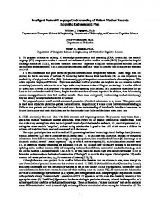
SRU CR and i = 1, 2, 3, ... The next conditions must be respected: - All non-terminals from si must be found one time and only one in qi. Terminals, pseudo-terminals and direct actions from si can be found at most one time in qi. - All terminals, pseudo-terminals and direct actions from qi must be found one time and only one in si. - Eventually, qi can be empty. If si, and/or qi contain the same non-terminal, terminal, pseudo-terminal, direct action, subordinate relation or coordinate relation many times, then the apparition of the same element will be differently labeled in order to distinguish them. - An ntpa can have zero or one output (i.e. a link oriented from the ntpa to other element) that goes to an sr or to a cr on fixed entries and zero, one or many inputs

(i.e. links from other elements that are oriented to the ntpa) that come from an sr. It will be noted by ntpa(i1, i2, …) or by ntpa() if no entry is available. - An sr has always an output that goes to an ntpa or to a cr on a supplementary entry and one input that comes from an ntpa or from a cr. It will be noted by sr(i1). - A cr can have zero or one output that goes to an sr or to a cr on fixed entry and can have m>=2 fixed inputs that come from ntpa or from cr and zero, one or many supplementary inputs that come from sr. It will be noted by cr(f1, f2,… / s1, s2, …) if it has supplementary inputs (where f1, f2, ... are fixed entries and s1, s2, ... are supplementary inputs) or by cr(f1, f2,…) if it has not supplementary inputs. We will consider m = 2 because this is used about correlative constructions that have two members. The ntpa-s and the links between them will constitute a dependency tree DT. The graphic notations to represent DT are showed in the figure 1. We can summarize the types of links as follows: 1. ntpa output -> sr input 2. ntpa output -> fixed cr input 3. sr output -> ntpa input 4. cr output -> sr input 5. cr output -> fixed cr input 6. sr output -> supplementary cr input An important feature of the DT is the head. A head in a DT is a node that has only inputs and has no output. An ntpa node can be head; it has inputs of type 3 (i.e. from sr relation). A cr node can be head; its fixed inputs are of type: 2 (from ntpa) and 5 (from other cr) and its supplementary inputs are of type 6 (from sr). An sr relation cannot be head. A dependency tree has one and only one head. A DT can be described using a BNF notation as follows: ::= | ::= ntpa()|ntpa() ::= ,| ::= sr() ::= ,| ::= cr(/)|cr() ::= ;| ::= ,| A dependency tree that do not contains non-terminals will be named final tree. Example: Let’s take an example that contains a gap: “I gave a book to the boy and a doll to the girl”. A grammar that can generate such a phrase is: (1) -> ( , ( @r1@( ()))) (2) -> ( “I”, “I”()) (3) -> ( , ( ())) (4) -> ( “gave”, “gave”()) (5) -> ( “and” , @r2@( (), () / @r3@( “and”())))

(6) -> ( , @r4@( (), ())) (7) -> ( , ()) (8) -> ( “a” , ( @r5@( “a”()))) (9) ->( “to” , “to”( @r6@(()))) (10) -> ( “the” , ( @r7@( “the”()))) (11) -> ( “book”, “book”()) (12) -> ( “boy”, “boy”()) (13) -> ( “doll”, “doll”()) (14) -> ( “girl”, “girl”())

"I"

@r1@

"gave"

"book

1 @r4@ 2

"to"

@r5@

"the"

@r6@

@r’5@

"a"

@r7@

"boy"

"a1"

@r2@ 1 2

"doll”

@r3@

"and

1 @r4@ 2

"to

"the1"

@r’6@

@r’7@

"girl"

Figure 2 – An example of DT

We noted by @r1@, @r2@, ... the relations. In a good description of a grammar these relations can have more appropriate names like: relation between subject and predicate, relation between article and noun, etc. For a certain natural language the number of the types of these relations cannot be too big. The relation @r4@ will be a special kind of relation (of the type cr – coordinate relation) that links together the two parts (direct part and indirect part) of this gap. We can name this relation a direct-indirect gap relation. Of course, other kinds of gap relations can be defined. The final DT for the phrase will be: “I”( @r1@( “gave”( @r2@( @r4@( “book”( @r5@( “a”)), “to”( @r6@(“boy”( @r7@( “the”()))))), @r’4@( “doll”( @r’5@( “a’”())), “to”( @r’6@( “girl”( @r’7@( “the1”()))))) / @r3@( “and”()))))) We will explain in the next sections how this final DT can be generated from the grammar. In the figure 2 we represented this final DT.

3 Non-Terminal Dependency Tree Substitution We will name non-terminal dependency tree a DT that has a non-terminal as head. We will name coordinate DT a DT that has a coordinate dependency as head. Let us take a non-terminal DT w that contains a non-terminal DT n = n’(u1, u2, ...)

where n’ is a non-terminal and u1, u2, ... are DTs that act as entries in the nonterminal n’. It is possible that n’ has no entries at all. It is possible too, that n’ have zero outputs (if it is a head of w) or one output that go somewhere in the tree w. To substitute n from w by a DT q means to obtain a new tree r that will replace n in w. If q = q’() is a DT without entries, then r = q’(). If q = q’(v1, v2, ...) is a nonterminal DT where q’ is a non-terminal and v1, v2, ... are dependency trees that act as entries in the non-terminal q’, then r = q’(u1, u2, ..., v1, v2, ...). If q = q’(v1, v2 / t1, t2, ...) is a coordinate relation DT where q’ is a coordinate relation, v1, v2, ... are DTs that act as entries in the fixed entries of the coordinate relation q’ and t1, t2, ... are DTs that act as entries in the supplementary entries of the coordinate relation q’ (it is possible that q’ has no supplementary inputs at all.), then r = q’(v1, v2 / t1, t2, ..., u1, u2, ...).

4 Generation in a Generative Dependency Grammar We consider 2 rules (i) ni->(si, qi) and (j) nj->(sj, qj) of a GDG. We consider also that si and qi contains pj. We will obtain a new rule (k) nk->(sk, qk) as follows: - sj will replace nj from si obtaining sk; - qj will substitute nj from qi obtaining qk; - nk = nj. We will say that the rule (k) is immediately generated from the rule (j) using the rule (i). Let us suppose that we have a phrase sn that contains only terminals. Let us suppose that, by applying a sequence of generations (starting with a rule that has a root symbol in the left side), we will obtain finally a rule (h) nh->(sh, qh) where sh is a phrase. We will consider too that in nh there are not non-terminals, pseudoterminals was replaced by matching terminals taken from the lexicon and direct actions was replaced by what results from their execution. The execution of a direct action has as result a terminal or a sequence of terminals that are considered as a single terminal. We will say that sh is completely generated by the grammar GDG (or that sh is accepted by the grammar GDG). In this case, qh will be the final dependency tree of the phrase sh. Remark: When a grammar rule is applied many times, all the elements of the rule are differently labeled for each application. Example: Using the grammar from the Example 1 (section 2) we can generate the DT as follows: (15)(1, 2) -> ( “I” , “I”( @r1@( ()))) (16)(15, 3) -> ( “I” , “I”( @r1@( ( ())))) (17)(16, 4) -> ( “I” “gave” , “I”( @r1@( “gave”( ())))) (18)(17, 5) -> ( “I” “gave” “and”, “I”( @r1@( “gave”( @r2@( (), () / @r3@( “and”())))))) We can continue the generation process and we will obtain finally:

(31)(30, 14) -> ( “I” “gave” “a” “book” “to” “the” “boy” “and” “a1” “doll”“to1” “the1” “girl”, “I”( @r1@( “gave”( @r2@( @r4@( “book”( @r5@( “a”())), “to”( @r6@(“boy” ( @r7@( “the”()))))), @r’4@( “doll”( @r5@( “a1”())), “to1”( @r’6@(“girl” ( @r’7@( “the1”()))))) / @r3@( and”())))))) In the right side of the rule we obtained the surface text “I” “gave” “a” “book” “to” “the” “boy” “and” “a1” “doll” “to1” “the1” “girl” and the DT (see the figure 2): “I”( @r1@( “gave”( @r2@( @r4@( “book”( @r5@( “a”())), “to”( @r6@(“boy” ( @r7@( “the”()))))), @r’4@( “doll”( @r5@( “a1”())), “to1”( @r’6@(“girl” ( @r’7@( “the1”()))))) / @r3@( and”())))))

5 GDG with Feature Structure One of the problem that arise when a GG is used is the great number of rules. This number can be controlled if we use a low number of metalinguistic symbols that can express a high number of linguistic situations. We will present such a formalism that is of type FS (feature structures). FS types are used for example in the PATR grammars (Shieber [14]) or in HPSG (Pollard [13]). In fact PATR or HPSG use AVM – Attribute Value Matrix. Instead of AVM we will define an AVT – Attribute Value Tree. We will consider also that the attribute are indexed or not indexed. If an attribute is indexed than in a certain context (for example in a grammar description rule) this attribute must take the same value for each ntpa that has associated the attribute. If an attribute is not indexed then in the same context this attribute can take any value from his value set. An AVT can be described syntactically as follows: 1. -> {:}|{}| 2. -> < indexed AVT >|< non indexed AVT > 3. -> [] 4. -> () 5. -> :|| 6. -> = 7. -> , | 8. -> | The rule 1 express the fact that an AVT can have a label – the AVT label definition. The AVT label can be used later alone in the same context and this mean that the label must be substituted with its definition. The rule 5 express the fact that an attribute with his list of values can have a label – the attribute list label definition. This label can be used later alone in the same context and this mean that the label must be substituted with its definition. In this case the label is also a marker for the attribute so two attributes with different labels (markers) must be considered as different attributes. Usually a context is formed by the left hand of a rule and one alternant from the right hand of the rule in a GG. The labels defined here are a sort of generalization of reentrancy from HPSG.

Definition: A GDG with feature structure is a GDG where each ntpa can have associated an AVT. The AVT associated with the non-terminal from the left side of the rules have always only indexed attributes. Example: Let us have the next statement in Romanian language: “Apele (the waters) linistite (still) sunt (are) adânci (deep)” that means “The still waters are deep”. We will not use all the grammatical categories implied in the analysis of this statement but only few as an illustration. We will consider that the lexical class (verb, adjective, noun, ...) will be represented also like an attribute “class“ that will have these values. Usually, the statement to be analyzed is first of all annotated i.e. each word will have attached his lemma and a particular AVT (that have only one value for each attribute. Each word can have many interpretations. For example “sunt” can represent the third person plural (are) or the first person singular (am). Though, for the sake of simplicity, we will consider only one interpretation for each word. The annotated statement will be: “Apele” apa[class = noun] [gender = feminine] [number = plural] “linistite” linistit [class = adjective] [gender = feminine] [number = plural] “sunt” fi [class = verb] [person: III] [number = plural] [mode = indicative] [voice = active] [time = present] “adânci” adânc [class = adjective] [gender = feminine] [number = plural] We noted in italics the lemmas. A GDG with features that can generate this statement can be as follows: (1) -> ( [gender = masculine, feminine, neuter] [number = singular, plural] [person = I, II, III] [gender = masculine, feminine, neuter] [number = singular, plural] [person = I, II, III], ( @r1@( ()))) (2) [gender = masculine, feminine, neuter] [number = singular, plural] [person = I, II, III] -> (%noun% [class = noun] [gender = masculine, feminine, neuter] [number = singular, plural] %adjective% [class = adjective] [gender = masculine, feminine, neuter] [number = singular, plural], %noun%(@r2@(%adjective% ()))) (3) [gender = masculine, feminine, neuter] [number = singular, plural] [person = I, II, III] -> (%verb% [class = verb] [gender = masculine, feminine, neuter] [number = singular, plural] [mode = indicative] [voice = active] [time = present, future, imperfect past] %adjective% [class = adjective] [gender = masculine, feminine, neuter] [number = singular, plural], %verb%(@r3@(%adjective% ()))) As we can see we used pseudo terminals for nouns, verbs, adjectives, so this grammar can generate a set of statements.

6 AVT Properties The labels are used in AVT only in order to reduce the length of the description. Before any AVT operation the labels must be substituted with their definition. During this substitution the eventually reccursivity must be identified. The reccursivity are not accepted.

AVT themselves are used also in order to represent more compactly a greater number of ntpa-s. How many such ntpa-s represent an AVT? The AVT associated with such an ntpa will be named EC (exclusive combination). An EC will have for each attribute only one value. We can compute how many paths are in an AVT, how these paths can be enumerated, how many EC-s are in an AVT and others proprieties. We explain here only how we can enumerate the EC-s in an AVT. In order to enumerate (generate) all the EC-s in an AVT we will use the notations

∏

(and “*”) that will mean “string concatenation” and

∑

(and “+”) that will

mean “string alternatives”. With these notations, the enumeration of the EC-s will be made with the next recursive formulas: - LES(T) =

∏ AES ( A ) k

is the set of EC (LES = List Exclusive Set) in an

k

AVT T that has on the first level an attribute list Ak. - AES(A) =

∑VES ( A / a ) is the set of EC-s that pass through the attribute A i

i

(AES = Attribute Exclusive Set) that has a list of values ai. - VES(A/a) =

∏ A / a * AES ( A ) is the set of EC-s that contain the attribute j

j

value a of the attribute A (VES = Value Exclusive Set) if a has associated an attribute list. If a has not associated an attribute list then VES(A/a)=A/a.

7 Logical Interpretation of an AVT We will give a logical interpretation of an AVT, i.e. a logical expression that correspond to an AVT. Using such an expression we can make in a more simple way some operations with AVT-s. In the enumeration of the EC-s we will consider that the sign “*” will represent the logical operation “and” and the sign “+” will represent the logical operation “or”. In this case LES(T) of an AVT T can be “read” as a logical expression. As in any ordinary logical expression we will have: a/a1 * a/a1 = a/a1 a/a1 + a/a1 = a/a1 and we will have all the others proprieties of the logical operators. Because (a/ai) and [a/ai] represent the indexing type, we will introduce also the next conventions: (a/ai) * (a/ai) = (a/ai) (a/ai) + [a/ai] = [a/ai] [a/ai] * (a/ai) = [a/ai] [a/ai] + [a/ai] = [a/ai] This means that the indexing has a priority against non indexing. Because an attribute can not have in the same time two different value we will consider: (a/ai) * [a/aj] = false (a/ai) * (a/aj) = false [a/ai] * (a/aj) = false

[a/ai] * [a/aj] = false where i #j and “false” as “true” have all the proprieties from logical expressions. The next rule must always be respected by a logical expression in order to be an AVT transformation: Each term of a disjunction must contain at least one factor that has the same attribute name. So, in each disjunction we must have something of the form: A/x1...+ A/x2...+ A/x3... + A/x4 ... We can use the logical representation of an AVT to make some operations and optimizations. Example S = [a = a1[b = b1, b2][c = c1, c2], a2(b = b1, b2)][e = e1, e2] LES(S) = [a/a1] * [b/b1] * [c/c1] * [e/e1] + [a/a1] * [b/b1] * [c/c2] * [e/e1] + [a/a1] * [b/b2] * [c/c1] * [e/e1] + [a/a1] * [b/b2] * [c/c2] * [e/e1] + [a/a2] * (b/b1) * [e/e1] + [a/a2] * (b/b2) * [e/e1] + [a/a1] * [b/b1] * [c/c1] * [e/e2] + [a/a1] * [b/b1] * [c/c2] * [e/e2] + [a/a1] * [b/b2] * [c/c1] * [e/e2] + [a/a1] * [b/b2] * [c/c2] * [e/e2] + [a/a2] * (b/b1) * [e/e2] + [a/a2] * (b/b2) * [e/e2] By applying different logical transformations we will obtain: LES(S) = ([a/a1] * ([c/c1] + [c/c2]) + [a/a2]) * ([b/b1] + [b/b2]) * ([e/e1] + [e/e2])

8 The Transformation of a Logical Expression into an AVT In the above section we explained how to obtain a logical expression representing an AVT. On this logical expression, some logical transformation can be executed. Finally, the logical expression can be transformed again in an AVT. We will show the method using the example from the section 7. We will consider as starting form that do not contains parenthesis and all the transformations described in 7 was applied. LES(S) = [a/a1] * [b/b1] * [c/c1] * [e/e1] + [a/a1] * [b/b1] * [c/c2] * [e/e1] + [a/a1] * [b/b2] * [c/c1] * [e/e1] + [a/a1] * [b/b2] * [c/c2] * [e/e1] + [a/a2] * [b/b1] * [e/e1] + [a/a2] * [b/b2] * [e/e1] + [a/a1] * [b/b1] * [c/c1] * [e/e2] + [a/a1] * [b/b1] * [c/c2] * [e/e2] + [a/a1] * [b/b2] * [c/c1] * [e/e2] + [a/a1] * [b/b2] * [c/c2] * [e/e2] + [a/a2] * [b/b1] * [e/e2] + [a/a2] * [b/b2] * [e/e2] a) We count the apparitions of each attribute in EC-s (an attribute can appear only one time in a EC because we considered the expression already simplified). In our case we will obtain: a: 12, b: 12, c: 8, e: 12 b) We count how many EC-s there are. Here we obtain 12. The attributes that appears in all the EC-s will be the attributes that will appear on the first level of the tree. In our case we will have something of the form: [a = ...] [b = ...]

[e = ...] We create a number of EC groups equal with the number of the EC-s that have the maximum number of apparitions. Each group contains all the EC-s from the expression. We consider that each group is associated with an attribute from those EC-s that had the apparition number equal with the number of EC-s from the current sub expression. LES(S) = ([a/a1] * [b/b1] * [c/c1] * [e/e1] + [a/a1] * [b/b1] * [c/c2] * [e/e1] + [a/a1] * [b/b2] * [c/c1] * [e/e1] + [a/a1] * [b/b2] * [c/c2] * [e/e1] + [a/a2] * [b/b1] * [e/e1] + [a/a2] * [b/b2] * [e/e1] + [a/a1] * [b/b1] * [c/c1] * [e/e2] + [a/a1] * [b/b1] * [c/c2] * [e/e2] + [a/a1] * [b/b2] * [c/c1] * [e/e2] + [a/a1] * [b/b2] * [c/c2] * [e/e2] + [a/a2] * [b/b1] * [e/e2] + [a/a2] * [b/b2] * [e/e2]) * ([a/a1] * [b/b1] * [c/c1] * [e/e1] + [a/a1] * [b/b1] * [c/c2] * [e/e1] + [a/a1] * [b/b2] * [c/c1] * [e/e1] + [a/a1] * [b/b2] * [c/c2] * [e/e1] + [a/a2] * [b/b1] * [e/e1] + [a/a2] * [b/b2] * [e/e1] + [a/a1] * [b/b1] * [c/c1] * [e/e2] + [a/a1] * [b/b1] * [c/c2] * [e/e2] + [a/a1] * [b/b2] * [c/c1] * [e/e2] + [a/a1] * [b/b2] * [c/c2] * [e/e2] + [a/a2] * [b/b1] * [e/e2] + [a/a2] * [b/b2] * [e/e2]) * ([a/a1] * [b/b1] * [c/c1] * [e/e1] + [a/a1] * [b/b1] * [c/c2] * [e/e1] + [a/a1] * [b/b2] * [c/c1] * [e/e1] + [a/a1] * [b/b2] * [c/c2] * [e/e1] + [a/a2] * [b/b1] * [e/e1] + [a/a2] * [b/b2] * [e/e1] + [a/a1] * [b/b1] * [c/c1] * [e/e2] + [a/a1] * [b/b1] * [c/c2] * [e/e2] + [a/a1] * [b/b2] * [c/c1] * [e/e2] + [a/a1] * [b/b2] * [c/c2] * [e/e2] + [a/a2] * [b/b1] * [e/e2] + [a/a2] * [b/b2] * [e/e2]) We can see that if we will develop this expression and we make some simplifications we will obtain the initial expression. c) From each EC of a group we will eliminate the attributes that are associated with others groups. LES(S) = ([a/a1] * [c/c1] + [a/a1] * [c/c2] + [a/a1] * [c/c1] + [a/a1] * [c/c2] + [a/a2] +[a/a2] + [a/a1] * [c/c1] + [a/a1] * [c/c2] + [a/a1] * [c/c1] + [a/a1] * [c/c2] + [a/a2] + [a/a2]) * ([b/b1] * [c/c1] + [b/b1] * [c/c2] + [b/b2] * [c/c1] + [b/b2] * [c/c2] + [b/b1] + [b/b2] + [b/b1] * [c/c1] + [b/b1] * [c/c2] + [b/b2] * [c/c1] + [b/b2] * [c/c2] + [b/b1] + [b/b2]) * ([e/e1] + [e/e1] + [e/e1] + [e/e1] + [e/e1] + [e/e1] + [e/e2] + [e/e2] + [e/e2] + [e/e2] + [e/e2] + [e/e2]) d) We will simplify the expressions from the parenthesis by keeping one sample from each combination and by applying transformations of the type x * y + x = x. LES(S) = ([a/a1] * [c/c1] + [a/a1] * [c/c2] + [a/a2]) * ([b/b1] + [b/b2]) * ([e/e1] + [e/e2]) e) In each group we take as common factor the attribute (and value) of the attribute associated with this group: LES(S) = ([a/a1] * ([c/c1] + [c/c2]) + [a/a2]) * ([b/b1] + [b/b2]) * ([e/e1] + [e/e2]) We will apply the steps (a) – (e) for each most inside parenthesis (for each attribute value). We continue this process until all the most inside parenthesis will contain only one attribute. In our case we already obtained the most inside parenthesis with only one attribute. f) We can transform now the expression in an AVT using the next procedure:

f1) For each sequence of the type ([x/x1] + [x/x2] + [x/x3] + ...) or ((x/x1) + (x/x2) + (x/x3) + ...) we apply the transformation [x = x1, x2, x3, ...] respectively (x = x1, x2, x3, ....). (Normally we can not have this kind of sequences with different index types, but anyway the index has a priority against not index). In our case we will have: S = ([a/a1] * [c = c1, c2] + [a/a2]) * [b = b1, b2] * [e = e1, e2] f2) For all the sequences of the type [x/x1] * (sequence) or (x/x1) * (sequence) we apply the transformation into [x/x1(sequence)] respectively (x/x1(sequence)). In our case we have: S = ([a/a1[c = c1, c2]] + [a/a2]) * [b = b1, b2] * [e = e1, e2] f3) For all the sequences of the type ([x/sequence1] + [x/sequence2] + [x/sequence3] + ...) or ((x/sequence1) + (x/sequence2) + (x/sequence3) + ...) we apply the transformation into [x = sequence1, sequence2, sequence3, ...] respectively (x = sequence1, sequence2, sequence3 ). In our case we have: S = [a = a1[c = c1, c2]], a2] * [b = b1, b2] * [e = e1, e2] f4) For all the sequences of the type [sequence1] * [sequence2] * [sequence3] ... we apply the transformation into [sequence1] [sequence2] [sequence3] ... . In our case we have: S= [a = a1[c = c1, c2]], a2] [b = b1, b2] [e = e1, e2] We obtained a well formed AVT.

9 The Unification We can define different operations/notions on the AVT: intersection (the common part of two AVT-s), difference (what it is in the first AVT and is not in the second AVT), sorted AVT (using total order relation on names of attributes and attribute values), AVT normalization (the “less deep” form of an AVT), etc. The most important operation is the unification that will make possible the substitution of a non-terminal from right side of a rule with a the rule that have in the left side the appropriate non-terminal. The substitution process is more complicated and we have not the space to fully explain it here. We will give only the definition of the unification. Definition: Two ntpa-s having associated AVT-s are unifiable if they have the same name and the unifier of the two AVT-s exists (i.e. it is not empty). (If the two ntpa-s have not associated AVT-s then they are unifiable only if they have the same name.) Definition: A unifier of two AVT-s is an AVT corresponding to an a expression obtained making a logical “and” between the logical forms of the two AVT-s. Example: Let us have two ntpa-s with the same name and with two AVT-s associated, S an T: S = [a = a1, a2, a3, a4] [b = b1, b2, b3] [c = c1, c2[f = f1][g = g1, g2]] [d = d1, d2[f = f2, f3][g = g1, g3, g4]] T = [c = c1[h = h1], c2, c3] [d = d1, d2[g = g3, g4, g5]] [e = e1, e2, e3, e4] The unifier R of S and T is R = S * T. We transform S and T in their logical form. We execute all the needed operations on the expression R * T. Finally, using the method described in section 8 we obtain:

R = [a = a1, a2, a3, a4] [b = b1, b2, b3] [c = c1] [h = h1] [d = d1[g = g3, g4], d2[f = f2, f3][g = g3, g4]] [e = e1, e2, e3, e4] The calculus can be complicated but it is not a problem to implement it in a computer program.

10 Conclusions We think that the GDG with feature structure have the power to represent the linguistic information and they do not imply an excessively difficulty to be used (tough it is not a trivial task to make a good description of a grammar). Using a GDG we can parse texts and obtain dependency trees associated to a source text. There are many directions in which GDG can be (and was) extended. For example we can define GDG with many DT-s in the right side of the rules. This will facilitate the description of the recursive rules. The GDG we defined uses a kind of relations that can be named direct relations because they link directly ntpas that are found in the current rule. We can define a more complicated sort of relations: indirect relations that link external ntpa to the current rule. These relations will facilitate too the writing of the grammar rules, especially for long distance relation between phrase parts, without the necessity to have all these parts in the same rule. There are at least few domains where these GDG can be used: the machine translation, the data retrieval, the language understanding. In the machine translation, these DT can describe relatively easily complex linguistic structures equivalences. In the data retrieval, on these DT can be formulated logical clauses that gather all the information from the source text. The number of the types of relations between the terminals and direct actions that we find in final dependency tree is not too big so a set of supplementary logical clauses can complete the grammar description. Using the clauses obtained from the final dependency trees and these supplementary clauses, complex inferences can be made on the dependency trees. We consider that the DT built by an analysis using GDG capture the “meaning” of the texts so it can serve to natural language understanding. Based on GDG formalism presented here we realized a specialized language GRAALAN (GRAmmar Abstract LANguage) that has a set of other features also. The logical and linguistic background of this language was defined and we presented in this paper only some elements of this background. Using GRAALAN we started to build a GDG with feature structure of the Romanian language. The Romanian language has a very difficult grammar with quite free word order. For example, only to express the accord between a multiple regent and a subordinate (in gender, number, animation, order) there are about 1350 situations that must be observed. We realized so far the description of the general rules for regent – subordinate relation (nominal – attributes, verbs – adjuncts, subjects - predicates) and we partially realized the description of nominal – attributes relation. References 1. Covington, Michael A. A Dependency Parser for Variable-Word-Order Languages, Research Report AI-1990-01, The University of Georgia, Athens, Georgia, 1990

2. Covington, Michael A. 1994 Discontinuous Dependency Parsing of Free and Fixed Word Order, Research Report AI-1992-02, The University of Georgia, Athens, Georgia, 1994 3. Bröker, Norbert How to define a context free backbone for DGs: Implementing a DG in the LFG formalism, Papers of the Workshop on the Processing of Dependency-based Grammars (COLING-ACL’98), 1998, pp.29-38 4. Chomsky, Noam Generative Grammar: Its Basis, Development and Prospects. Studies in English Linguistics and Literature, Special Issue, Kyoto University of Foreign Studies, 1988 5. Gaifman, H. Dependency Systems and phrase structure systems, Information and Control, 1965, pp. 304-337 6. Helwig, P. Chart Parsing according to the slot and filler principle, Processing of the 12th Int. Conf. On Computational Linguistics, Budapest, Hungary, 22-27 August 1988, Vol.1, 1988, pp. 242-244 7. Hudson, R English Word Grammar, Oxford UK, Basil Blackwell, 1990 8. McCord, M Slot grammar: A system for simpler construction of practical natural language grammars, in R. Studer (Ed.), Natural Language and Logic, Berlin Heidelberg Springer, 1990, pp.118-145 9. Kahane, Sylvain, Alexis Nasr, and Owen Rambow Pseudo-projectivity: A polynomially parsable nonprojective dependency grammar. In Proceedings of the 36th Annual Meeting of the Association for Computational Linguistics (ACL '98), Montreal, Canada, 1998 10. Mel'cuk, I.A., Pertsov, N.V. Surface Syntax of English: A formal model within the Meaning-Text Framework, Amsterdam/PA: John Benjamins, 1987 11. Mel’cuk, I.A. Dependency Syntax: theory and practice, State University of New York Press, Albany, 1988 12. Milward, D. Dynamic Dependency Grammar, Linguistics and Philosophy 17, December, 1994, pp. 561-606 13. Pollard, C. Sag, I. A. Head-driven Phrase Structure grammar, University of Chicago Press and Standford CSLI Publications, 1994 14. Shieber, Stuart M. An Introduction to Unification Based Approaches to Grammar, CLSII Lecture Notes Series, Number 4, Center for the study of Language and Information, Stanford University, 1986 15. Starosta, S Lexicase revisited. Department of Linguistics, University of Hawaii, 1992 16. Teich, Elke Types of syntagmatic grammatical relations and their representation, Papers of the Workshop on the Processing of Dependency-based Grammars (COLINGACL’98), 1998, pp.39-48 17. Tesnière, L. Éléments de syntaxe structurelle, Paris, Klincksieck, 1959