Nature-Inspired Metaheuristic Algorithms, 2nd Edition by Xin-She Yang. Copyright cO ...... The flashing light of fireflies is an amazing sight in the summer sky in.
Nature-Inspired Metaheuristic Algorithms Second Edition
Xin-She Yang
d Me
ta h e u r is
ti
lgorith m s
N a t u re -I n s
i re
cA
p
University of Cambridge, United Kingdom
Xin-She Yang
10
S ec
on
)
c
Luniver Press
d E d ion (20 it
Luniver Press
Published in 2010 by Luniver Press Frome, BA11 6TT, United Kingdom www.luniver.com c Copyright °Luniver Press 2010 c Copyright °Xin-She Yang 2010 All rights reserved. This book, or parts thereof, may not be reproduced in any form or by any means, electronic or mechanical, including photocopying, recording or by any information storage and retrieval system, without permission in writing from the copyright holder.
British Library Cataloguing-in-Publication Data A catalogue record for this book is available from the British Library
ISBN-13: 978-1-905986-28-6 ISBN-10: 1-905986-28-9
d Me
ta h e u r is
ti
lgorith m s
N a t u re -I n s
i re
cA
p
While every attempt is made to ensure that the information in this publication is correct, no liability can be accepted by the authors or publishers for loss, damage or injury caused by any errors in, or omission from, the information given.
Xin-She Yang
10
S ec
on
)
c
Luniver Press
d E d ion (20 it
CONTENTS
Preface to the Second Edition
v
Preface to the First Edition
vi
1
Introduction
1
1.1 1.2 1.3 1.4
1 2 4 5
ti
Xin-She Yang
10
S ec
)
c
Luniver Press
on
Random Walks and L´ evy Flights
11
2.1 2.2 2.3 2.4
11 12 14 17
lgorith m s
N a t u re -I n s
e ta h e u r is
cA
p
2
dM i re
d E d ion (20 it
Optimization Search for Optimality Nature-Inspired Metaheuristics A Brief History of Metaheuristics
Random Variables Random Walks L´evy Distribution and L´evy Flights Optimization as Markov Chains
i
ii
3
4
5
6
7
CONTENTS
Simulated Annealing
21
3.1 3.2 3.3 3.4 3.5
21 22 23 24 26
How to Deal With Constraints
29
4.1 4.2 4.3 4.4 4.5
29 32 33 34 35
p
ta h e u r is
ti
cA
lgorith m s
N a t u re -I n s
d Me
Xin-She Yang
10
S ec
on
)
c
Luniver Press
d E d ion (20 it
Method of Lagrange Multipliers Penalty Method Step Size in Random Walks Welded Beam Design SA Implementation
Genetic Algorithms
41
5.1 5.2 5.3
41 42 43
Introduction Genetic Algorithms Choice of Parameters
Differential Evolution
47
6.1 6.2 6.3 6.4
47 47 50 50
Introduction Differential Evolution Variants Implementation
Ant and Bee Algorithms
53
7.1
53 53 54 56 57 57 57 58 59 60 61
7.2 i re
Annealing and Boltzmann Distribution Parameters SA Algorithm Unconstrained Optimization Stochastic Tunneling
Ant Algorithms 7.1.1 Behaviour of Ants 7.1.2 Ant Colony Optimization 7.1.3 Double Bridge Problem 7.1.4 Virtual Ant Algorithm Bee-inspired Algorithms 7.2.1 Behavior of Honeybees 7.2.2 Bee Algorithms 7.2.3 Honeybee Algorithm 7.2.4 Virtual Bee Algorithm 7.2.5 Artificial Bee Colony Optimization
CONTENTS
8
9
10
11
Swarm Optimization
63
8.1 8.2 8.3 8.4 8.5
63 64 65 66 69 73
9.1 9.2 9.3
73 74 76 81
10.1 10.2 10.3 10.4 10.5 10.6 10.7
81 82 83 84 86 89 89
p
ti
cA
Xin-She Yang
) 10
S ec
d E d ion (20 it
Echolocation of bats 11.1.1 Behaviour of microbats 11.1.2 Acoustics of Echolocation Bat Algorithm 11.2.1 Movement of Virtual Bats 11.2.2 Loudness and Pulse Emission Validation and Discussions Implementation Further Topics
97 97 97 98 98 99 100 101 102 103
Cuckoo Search
105
12.1 12.2 12.3 12.4
105 106 106 108
lgorith m s
N a t u re -I n s
12
c
Luniver Press
on
Behaviour of Fireflies Firefly Algorithm Light Intensity and Attractiveness Scalings and Asymptotics Implementation FA variants Spring Design
Bat Algorithm
11.3 11.4 11.5
ta h e u r is
Harmonics and Frequencies Harmony Search Implementation
Firefly Algorithm
11.2
d Me
Swarm Intelligence PSO algorithms Accelerated PSO Implementation Convergence Analysis
Harmony Search
11.1
i re
iii
Cuckoo Breeding Behaviour L´evy Flights Cuckoo Search Choice of Parameters
iv
CONTENTS
12.5 13
117
13.1
117 117 118 119 121 121 121 122 125 127
14.1 14.2 14.3 14.4 14.5
127 128 130 133 135 135 135 136 137 137 137
p
ta h e u r is
141
Index
147
ti
lgorith m s
Xin-She Yang
10
S ec
)
c
Luniver Press
on
Intensification and Diversification Ways for Intensification and Diversification Generalized Evolutionary Walk Algorithm (GEWA) Eagle Strategy Other Metaheuristic Algorithms 14.5.1 Tabu Search 14.5.2 Photosynthetic and Enzyme Algorithm 14.5.3 Artificial Immune System and Others Further Research 14.6.1 Open Problems 14.6.2 To be Inspired or not to be Inspired
References
cA
N a t u re -I n s
d Me
Artificial Neural Networks 13.1.1 Artificial Neuron 13.1.2 Neural Networks 13.1.3 Back Propagation Algorithm Support Vector Machine 13.2.1 Classifications 13.2.2 Statistical Learning Theory 13.2.3 Linear Support Vector Machine 13.2.4 Kernel Functions and Nonlinear SVM
Metaheuristics – A Unified Approach
14.6
i re
108
ANNs and Support Vector Machine
13.2
14
Implementation
d E d ion (20 it
v
Preface to the Second Edition Since the publication of the first edition of this book in 2008, significant developments have been made in metaheuristics, and new nature-inspired metaheuristic algorithms emerge, including cuckoo search and bat algorithms. Many readers have taken time to write to me personally, providing valuable feedback, asking for more details of algorithm implementation, or simply expressing interests in applying these new algorithms in their applications. In this revised edition, we strive to review the latest developments in metaheuristic algorithms, to incorporate readers’ suggestions, and to provide a more detailed description to algorithms. Firstly, we have added detailed descriptions of how to incorporate constraints in the actual implementation. Secondly, we have added three chapters on differential evolution, cuckoo search and bat algorithms, while some existing chapters such as ant algorithms and bee algorithms are combined into one due to their similarity. Thirdly, we also explained artificial neural networks and support vector machines in the framework of optimization and metaheuristics. Finally, we have been trying in this book to provide a consistent and unified approach to metaheuristic algorithms, from a brief history in the first chapter to the unified approach in the last chapter. Furthermore, we have provided more Matlab programs. At the same time, we also omit some of the implementation such as genetic algorithms, as we know that there are many good software packages (both commercial and open course). This allows us to focus more on the implementation of new algorithms. Some of the programs also have a version for constrained optimization, and readers can modify them for their own applications. Even with the good intention to cover most popular metaheuristic algorithms, the choice of algorithms is a difficult task, as we do not have the space to cover every algorithm. The omission of an algorithm does not mean that it is not popular. In fact, some algorithms are very powerful and routinely used in many applications. Good examples are Tabu search and combinatorial algorithms, and interested readers can refer to the references provided at the end of the book. The effort in writing this little book becomes worth while if this book could in some way encourage readers’ interests in metaheuristics.
d Me
ta h e u r is
August 2010
ti
lgorith m s
N a t u re -I n s
i re
cA
p
Xin-She Yang
Xin-She Yang
10
S ec
on
)
c
Luniver Press
d E d ion (20 it
Chapter 1
INTRODUCTION It is no exaggeration to say that optimization is everywhere, from engineering design to business planning and from the routing of the Internet to holiday planning. In almost all these activities, we are trying to achieve certain objectives or to optimize something such as profit, quality and time. As resources, time and money are always limited in real-world applications, we have to find solutions to optimally use these valuable resources under various constraints. Mathematical optimization or programming is the study of such planning and design problems using mathematical tools. Nowadays, computer simulations become an indispensable tool for solving such optimization problems with various efficient search algorithms. 1.1
OPTIMIZATION
Mathematically speaking, it is possible to write most optimization problems in the generic form minimize x∈ 0 is a parameter which is the mean or expectation of the occurrence of the event during a unit interval. Xin-She Yang Different random variables will have different distributions. Gaussian c
Luniver Press distribution or normal distribution is by far the most popular distribuon 20 d E d i otions, because many physical variables including light intensity, and erit n ( i re
Nature-Inspired Metaheuristic Algorithms, 2nd Edition by Xin-She Yang c 2010 Luniver Press Copyright °
11
12
´ CHAPTER 2. RANDOM WALKS AND LEVY FLIGHTS
rors/uncertainty in measurements, and many other processes obey the normal distribution p(x; µ, σ 2 ) =
1 (x − µ)2 √ exp[− ], 2σ 2 σ 2π
−∞ < x < ∞,
(2.2)
where µ is the mean and σ > 0 is the standard deviation. This normal distribution is often denoted by N(µ, σ 2 ). In the special case when µ = 0 and σ = 1, it is called a standard normal distribution, denoted by N(0, 1). In the context of metaheuristics, another important distribution is the so-called L´evy distribution, which is a distribution of the sum of N identically and independently distribution random variables whose Fourier transform takes the following form FN (k) = exp[−N |k|β ].
(2.3)
The inverse to get the actual distribution L(s) is not straightforward, as the integral Z β 1 ∞ L(s) = cos(τ s)e−α τ dτ, (0 < β ≤ 2), (2.4) π 0 does not have analytical forms, except for a few special cases. Here L(s) is called the L´evy distribution with an index β. For most applications, we can set α = 1 for simplicity. Two special cases are β = 1 and β = 2. When β = 1, the above integral becomes the Cauchy distribution. When β = 2, it becomes the normal distribution. In this case, L´evy flights become the standard Brownian motion. Mathematically speaking, we can express the integral (2.4) as an asymptotic series, and its leading-order approximation for the flight length results in a power-law distribution L(s) ∼ |s|−1−β ,
(2.5)
which is heavy-tailed. The variance of such a power-law distribution is infinite for 0 < β < 2. The moments diverge (or are infinite) for 0 < β < 2, which is a stumbling block for mathematical analysis.
e ta h e u r is
A random walk is a random process which consists of taking a series of random steps. Mathematically speaking, let SN denotes the sum of each consecutive random step Xi , then SN forms a random walk
ti consecutive lgorith m s
N a t u re -I n s
dM i re
Xin-She Yang
10
S ec
)
c
Luniver Press
on
RANDOM WALKS
cA
p
2.2
d E d ion (20 it
SN =
N X i=1
Xi = X1 + ... + XN ,
(2.6)
2.2 RANDOM WALKS
13
where Xi is a random step drawn from a random distribution. This relationship can also be written as a recursive formula SN =
N −1 X
+XN = SN −1 + XN ,
(2.7)
i=1
which means the next state SN will only depend the current existing state SN −1 and the motion or transition XN from the existing state to the next state. This is typically the main property of a Markov chain to be introduced later. Here the step size or length in a random walk can be fixed or varying. Random walks have many applications in physics, economics, statistics, computer sciences, environmental science and engineering. Consider a scenario, a drunkard walks on a street, at each step, he can randomly go forward or backward, this forms a random walk in onedimensional. If this drunkard walks on a football pitch, he can walk in any direction randomly, this becomes a 2D random walk. Mathematically speaking, a random walk is given by the following equation St+1 = St + wt ,
(2.8)
where St is the current location or state at t, and wt is a step or random variable with a known distribution. If each step or jump is carried out in the n-dimensional space, the random walk discussed earlier SN =
N X
Xi ,
(2.9)
i=1
d Me
ta h e u r is
ti
lgorith m s
N a t u re -I n s
i re
cA
p
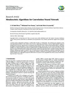
becomes a random walk in higher dimensions. In addition, there is no reason why each step length should be fixed. In fact, the step size can also vary according to a known distribution. If the step length obeys the Gaussian distribution, the random walk becomes the Brownian motion (see Fig. 2.1). In theory, as the number of steps N increases, the central limit theorem implies that the random walk (2.9) should approaches a Gaussian distribution. As the mean of particle locations shown in Fig. 2.1 is obviously zero, their variance will increase linearly with t. In general, in the d-dimensional space, the variance of Brownian random walks can be written as σ 2 (t) = |v0 |2 t2 + (2dD)t,
(2.10)
where v0 is the drift velocity of the system. Here D = s2 /(2τ ) is the effective diffusion coefficient which is related to the step length s over a on 20 d E d i oshort time interval τ during each jump. it n ( Xin-She Yang
10
S ec
)
c
Luniver Press
´ CHAPTER 2. RANDOM WALKS AND LEVY FLIGHTS
14
s
Figure 2.1: Brownian motion in 2D: random walk with a Gaussian step-size distribution and the path of 50 steps starting at the origin (0, 0) (marked with •).
Therefore, the Brownian motion B(t) essentially obeys a Gaussian distribution with zero mean and time-dependent variance. That is, B(t) ∼ N (0, σ 2 (t)) where ∼ means the random variable obeys the distribution on the right-hand side; that is, samples should be drawn from the distribution. A diffusion process can be viewed as a series of Brownian motion, and the motion obeys the Gaussian distribution. For this reason, standard diffusion is often referred to as the Gaussian diffusion. If the motion at each step is not Gaussian, then the diffusion is called non-Gaussian diffusion. If the step length obeys other distribution, we have to deal with more generalized random walk. A very special case is when the step length obeys the L´evy distribution, such a random walk is called a L´evy flight or L´evy walk. ´ ´ LEVY DISTRIBUTION AND LEVY FLIGHTS
2.3
Broadly speaking, L´evy flights are a random walk whose step length is drawn from the L´evy distribution, often in terms of a simple power-law formula L(s) ∼ |s|−1−β where 0 < β ≤ 2 is an index. Mathematically speaking, a simple version of L´evy distribution can be defined as
L(s, γ, µ) =
p γ γ 1 2π exp[− 2(s−µ) ] (s−µ)3/2 ,
0
0 0 such as f ← f + A if necessary. By constructing a Markov chain Monte Carlo, we can formulate a generic framework as outlined by Ghate and Smith in 2008, as shown in Figure 2.3. In this framework, simulated annealing and its many variants are simply a special case with ∆f exp[− Tt ] if ft+1 > ft , Pt = 1 if ft+1 ≤ ft
10
p
S ec
)
lgorith m s
N a t u re -I n s
cA
In this case, only the difference ∆f between the function values is important. Algorithms such as simulated annealing, to be discussed in the next chapter, use a single Markov chain, which may not be very efficient. In practice, it is usually advantageous to use multiple Markov chains in parallel to increase the overall efficiency. In fact, the algorithms such as particle swarm optimization can be viewed as multiple interacting Markov chains, though such theoretical analysis remains almost intractable. The theory of ta h d M e eu ris ti interacting Markov chains is complicated and yet still under development, i re however, any progress in such areas will play a central role in the underXin-She Yang standing how population- and trajectory-based metaheuristic algorithms c
Luniver Press perform under various conditions. However, even though we do not fully on d E d i o n ( 2 0understand why metaheuristic algorithms work, this does not hinder us to it
2.4 OPTIMIZATION AS MARKOV CHAINS
19
Markov Chain Algorithm for Optimization Start with ζ0 ∈ S, at t = 0 while (criterion) Propose a new solution Yt+1 ; Generate a random number 0 ≤ Pt ≤ 1; ½ Yt+1 with probability Pt ζt+1 = ζt with probability 1 − Pt
(2.27)
end Figure 2.3: Optimization as a Markov chain.
use these algorithms efficiently. On the contrary, such mysteries can drive and motivate us to pursue further research and development in metaheuristics.
REFERENCES 1. W. J. Bell, Searching Behaviour: The Behavioural Ecology of Finding Resources, Chapman & Hall, London, (1991). 2. C. Blum and A. Roli, Metaheuristics in combinatorial optimization: Overview and conceptural comparison, ACM Comput. Surv., 35, 268-308 (2003). 3. G. S. Fishman, Monte Carlo: Concepts, Algorithms and Applications, Springer, New York, (1995). 4. D. Gamerman, Markov Chain Monte Carlo, Chapman & Hall/CRC, (1997). 5. L. Gerencser, S. D. Hill, Z. Vago, and Z. Vincze, Discrete optimization, SPSA, and Markov chain Monte Carlo methods, Proc. 2004 Am. Contr. Conf., 3814-3819 (2004). 6. C. J. Geyer, Practical Markov Chain Monte Carlo, Statistical Science, 7, 473-511 (1992). 7. A. Ghate and R. Smith, Adaptive search with stochastic acceptance probabilities for global optimization, Operations Research Lett., 36, 285-290 (2008).
9. M. Gutowski, L´evy flights as an underlying mechanism for global optimizati tion algorithms, ArXiv Mathematical Physics e-Prints, June, (2001).
e ta h e u r is
10. W. K. Hastings, Monte Carlo sampling methods using Markov chains and their applications, Biometrika, 57, 97-109 (1970).
Xin-She Yang
lgorith m s
N a t u re -I n s
dM i re
cA
p
8. W. R. Gilks, S. Richardson, and D. J. Spiegelhalter, Markov Chain Monte Carlo in Practice, Chapman & Hall/CRC, (1996).
c
Luniver Press
)
11. S. Kirkpatrick, C. D. Gellat and M. P. Vecchi, Optimization by simulated 10
S ec
on
d E d i o n ( 2 0 annealing, Science, 220, 670-680 (1983). it
20
´ CHAPTER 2. RANDOM WALKS AND LEVY FLIGHTS
12. R. N. Mantegna, Fast, accurate algorithm for numerical simulation of Levy stable stochastic processes, Physical Review E, 49, 4677-4683 (1994). 13. E. Marinari and G. Parisi, Simulated tempering: a new Monte Carlo scheme, Europhysics Lett., 19, 451-458 (1992). 14. J. P. Nolan, Stable distributions: models for heavy-tailed data, American University, (2009). 15. N. Metropolis, and S. Ulam, The Monte Carlo method, J. Amer. Stat. Assoc., 44, 335-341 (1949). 16. N. Metropolis, A. W. Rosenbluth, M. N. Rosenbluth, A. H. Teller, and E. Teller, Equation of state calculations by fast computing machines, J. Chem. Phys., 21, 1087-1092 (1953). 17. I. Pavlyukevich, L´evy flights, non-local search and simulated annealing, J. Computational Physics, 226, 1830-1844 (2007). 18. G. Ramos-Fernandez, J. L. Mateos, O. Miramontes, G. Cocho, H. Larralde, B. Ayala-Orozco, L´evy walk patterns in the foraging movements of spider monkeys (Ateles geoffroyi),Behav. Ecol. Sociobiol., 55, 223-230 (2004). 19. A. M. Reynolds and M. A. Frye, Free-flight odor tracking in Drosophila is consistent with an optimal intermittent scale-free search, PLoS One, 2, e354 (2007). 20. A. M. Reynolds and C. J. Rhodes, The L´evy flight paradigm: random search patterns and mechanisms, Ecology, 90, 877-887 (2009). 21. I. M. Sobol, A Primer for the Monte Carlo Method, CRC Press, (1994). 22. M. E. Tipping M. E., Bayesian inference: An introduction to principles and and practice in machine learning, in: Advanced Lectures on Machine Learning, O. Bousquet, U. von Luxburg and G. Ratsch (Eds), pp.41-62 (2004). 23. G. M. Viswanathan, S. V. Buldyrev, S. Havlin, M. G. E. da Luz, E. P. Raposo, and H. E. Stanley, L´evy flight search patterns of wandering albatrosses, Nature, 381, 413-415 (1996).
d Me
ta h e u r is
ti
lgorith m s
N a t u re -I n s
i re
cA
p
24. E. Weisstein, http://mathworld.wolfram.com
Xin-She Yang
10
S ec
on
)
c
Luniver Press
d E d ion (20 it
Chapter 3
SIMULATED ANNEALING One of the earliest and yet most popular metaheuristic algorithms is simulated annealing (SA), which is a trajectory-based, random search technique for global optimization. It mimics the annealing process in material processing when a metal cools and freezes into a crystalline state with the minimum energy and larger crystal size so as to reduce the defects in metallic structures. The annealing process involves the careful control of temperature and its cooling rate, often called annealing schedule.
3.1
ANNEALING AND BOLTZMANN DISTRIBUTION
10
p
S ec
)
lgorith m s
N a t u re -I n s
cA
Since the first development of simulated annealing by Kirkpatrick, Gelatt and Vecchi in 1983, SA has been applied in almost every area of optimization. Unlike the gradient-based methods and other deterministic search methods which have the disadvantage of being trapped into local minima, the main advantage of simulated annealing is its ability to avoid being trapped in local minima. In fact, it has been proved that simulated annealing will converge to its global optimality if enough randomness is used in combination with very slow cooling. Essentially, simulated annealing is a search algorithm via a Markov chain, which converges under appropriate conditions. Metaphorically speaking, this is equivalent to dropping some bouncing balls over a landscape, and as the balls bounce and lose energy, they settle down to some local minima. If the balls are allowed to bounce enough times and lose energy slowly enough, some of the balls will eventually fall into the globally lowest locations, hence the global minimum will be reached. The basic idea of the simulated annealing algorithm is to use random search in terms of a Markov chain, which not only accepts changes that ta h u r is d M e eimprove ti the objective function, but also keeps some changes that are not i re ideal. In a minimization problem, for example, any better moves or changes Xin-She Yang that decrease the value of the objective function f will be accepted; howc
Luniver Press ever, some changes that increase f will also be accepted with a probability on 20 d E d i op. i t n ( This probability p, also called the transition probability, is determined Nature-Inspired Metaheuristic Algorithms, 2nd Edition by Xin-She Yang c 2010 Luniver Press Copyright °
21
22
CHAPTER 3. SIMULATED ANNEALING
by p=e
− k∆ET B
,
(3.1)
where kB is the Boltzmann’s constant, and for simplicity, we can use k to denote kB because k = 1 is often used. T is the temperature for controlling the annealing process. ∆E is the change of the energy level. This transition probability is based on the Boltzmann distribution in statistical mechanics. The simplest way to link ∆E with the change of the objective function ∆f is to use ∆E = γ∆f, (3.2) where γ is a real constant. For simplicity without losing generality, we can use kB = 1 and γ = 1. Thus, the probability p simply becomes p(∆f, T ) = e−∆f /T .
(3.3)
Whether or not we accept a change, we usually use a random number r as a threshold. Thus, if p > r, or ∆f
p = e− T > r,
(3.4)
the move is accepted. 3.2
PARAMETERS
10
p
S ec
)
lgorith m s
N a t u re -I n s
cA
Here the choice of the right initial temperature is crucially important. For a given change ∆f , if T is too high (T → ∞), then p → 1, which means almost all the changes will be accepted. If T is too low (T → 0), then any ∆f > 0 (worse solution) will rarely be accepted as p → 0 and thus the diversity of the solution is limited, but any improvement ∆f will almost always be accepted. In fact, the special case T → 0 corresponds to the gradient-based method because only better solutions are accepted, and the system is essentially climbing up or descending along a hill. Therefore, if T is too high, the system is at a high energy state on the topological landscape, and the minima are not easily reached. If T is too low, the system may be trapped in a local minimum (not necessarily the global minimum), and there is not enough energy for the system to jump out the local minimum to explore other minima including the global minimum. So ta h d M e eu ris ti a proper initial temperature should be calculated. i re Another important issue is how to control the annealing or cooling proXin-She Yang cess so that the system cools down gradually from a higher temperature c
Luniver Press to ultimately freeze to a global minimum state. There are many ways of on d E d i o n ( 2 0controlling the cooling rate or the decrease of the temperature. it
3.3 SA ALGORITHM
23
Two commonly used annealing schedules (or cooling schedules) are: linear and geometric. For a linear cooling schedule, we have T = T0 − βt,
(3.5)
or T → T − δT , where T0 is the initial temperature, and t is the pseudo time for iterations. β is the cooling rate, and it should be chosen in such a way that T → 0 when t → tf (or the maximum number N of iterations), this usually gives β = (T0 − Tf )/tf . On the other hand, a geometric cooling schedule essentially decreases the temperature by a cooling factor 0 < α < 1 so that T is replaced by αT or T (t) = T0 αt , t = 1, 2, ..., tf . (3.6) The advantage of the second method is that T → 0 when t → ∞, and thus there is no need to specify the maximum number of iterations. For this reason, we will use this geometric cooling schedule. The cooling process should be slow enough to allow the system to stabilize easily. In practise, α = 0.7 ∼ 0.99 is commonly used. In addition, for a given temperature, multiple evaluations of the objective function are needed. If too few evaluations, there is a danger that the system will not stabilize and subsequently will not converge to its global optimality. If too many evaluations, it is time-consuming, and the system will usually converge too slowly, as the number of iterations to achieve stability might be exponential to the problem size. Therefore, there is a fine balance between the number of evaluations and solution quality. We can either do many evaluations at a few temperature levels or do few evaluations at many temperature levels. There are two major ways to set the number of iterations: fixed or varied. The first uses a fixed number of iterations at each temperature, while the second intends to increase the number of iterations at lower temperatures so that the local minima can be fully explored.
dM
The simulated annealing algorithm can be summarized as the pseudo code shown in Fig. 3.1. In order to find a suitable starting temperature T0 , we can use any information about the objective function. If we know the maximum change max(∆f ) of the objective function, we can use this to estimate an initial temperature T0 for a given probability p0 . That is e ta h e u r is t
i
lgorith m s
N a t u re -I n s
i re
SA ALGORITHM
cA
p
3.3
Xin-She Yang
c
Luniver Press
max(∆f ) . ln p0
)
If we do not know the possible maximum change of the objective function, can use a heuristic approach. We can start evaluations from a very 10
S ec
on
T0 ≈ −
20 d E d i owe it n (
24
CHAPTER 3. SIMULATED ANNEALING
Simulated Annealing Algorithm Objective function f (x), x = (x1 , ..., xp )T Initialize initial temperature T0 and initial guess x(0) Set final temperature Tf and max number of iterations N Define cooling schedule T 7→ αT , (0 < α < 1) while ( T > Tf and n < N ) Move randomly to new locations: xn+1 = xn + ² (random walk) Calculate ∆f = fn+1 (xn+1 ) − fn (xn ) Accept the new solution if better if not improved Generate a random number r Accept if p = exp[−∆f /T ] > r end if Update the best x∗ and f∗ n=n+1 end while Figure 3.1: Simulated annealing algorithm.
high temperature (so that almost all changes are accepted) and reduce the temperature quickly until about 50% or 60% of the worse moves are accepted, and then use this temperature as the new initial temperature T 0 for proper and relatively slow cooling. For the final temperature, it should be zero in theory so that no worse move can be accepted. However, if Tf → 0, more unnecessary evaluations are needed. In practice, we simply choose a very small value, say, Tf = 10−10 ∼ 10−5 , depending on the required quality of the solutions and time constraints. 3.4
UNCONSTRAINED OPTIMIZATION
d Me
ta h e u r is
ti
lgorith m s
N a t u re -I n s
i re
cA
p
Based on the guidelines of choosing the important parameters such as the cooling rate, initial and final temperatures, and the balanced number of iterations, we can implement the simulated annealing using both Matlab and Octave. For Rosenbrock’s banana function f (x, y) = (1 − x)2 + 100(y − x2 )2 ,
we know that its global minimum f∗ = 0 occurs at (1, 1) (see Fig. 3.2). This is a standard test function and quite tough for most algorithms. However, on d E d i o n ( 2 0by modifying the program given later in the next chapter, we can find this it Xin-She Yang
10
S ec
)
c
Luniver Press
3.4 UNCONSTRAINED OPTIMIZATION
25
2 1 0 -1 -2 -2
-1
0
1
2
Figure 3.2: Rosenbrock’s function with the global minimum f∗ = 0 at (1, 1).
Figure 3.3: 500 evaluations during the annealing iterations. The final global best is marked with •.
10
p
S ec
)
lgorith m s
N a t u re -I n s
cA
global minimum easily and the last 500 evaluations during annealing are shown in Fig. 3.3. ta h d M e eu ris ti This banana function is still relatively simple as it has a curved nari re row valley. We should validate SA against a wide range of test functions, Xin-She Yang especially those that are strongly multimodal and highly nonlinear. It is c
Luniver Press straightforward to extend the above program to deal with highly nonlinear on 20 d E d i omultimodal functions. it n (
26
CHAPTER 3. SIMULATED ANNEALING
f (x)
g(x)
Figure 3.4: The basic idea of stochastic tunneling by transforming f (x) to g(x), suppressing some modes and preserving the locations of minima.
3.5
STOCHASTIC TUNNELING
To ensure the global convergence of simulated annealing, a proper cooling schedule must be used. In the case when the functional landscape is complex, simulated annealing may become increasingly difficult to escape the local minima if the temperature is too low. Raising the temperature, as that in the so-called simulated tempering, may solve the problem, but the convergence is typically slow, and the computing time also increases. Stochastic tunneling uses the tunneling idea to transform the objective function landscape into a different but more convenient one (e.g., Wenzel and Hamacher, 1999). The essence is to construct a nonlinear transformation so that some modes of f (x) are suppressed and other modes are amplified, while preserving the loci of minima of f (x). The standard form of such a tunneling transformation is g(x) = 1 − exp[−γ(f (x) − f0 )],
(3.7)
10
p
S ec
)
lgorith m s
N a t u re -I n s
cA
where f0 is the current lowest value of f (x) found so far. γ > 0 is a scaling parameter, and g is the transformed new landscape. From this simple transformation, we can see that g → 0 when f − f0 → 0, that is when f0 is approaching the true global minimum. On the other hand, if f À f0 , then g → 1, which means that all the modes well above the current minimum f0 are suppressed. For a simple one-dimensional function, it is easy to see that such properties indeed preserve the loci of the function (see Fig. 3.4). As the loci of the minima are preserved, then all the modes that above the current lowest value f0 are suppressed to some degree, while the modes below f0 are expanded or amplified, which makes it easy for the system to ta h d M e eu ris ti escape local modes. Simulations and studies suggest that it can significantly i re improve the convergence for functions with complex landscape and modes. Xin-She Yang Up to now we have not actually provided a detailed program to show c
Luniver Press how the SA algorithm can be implemented in practice. However, before on d E d i o n ( 2 0we can actually do this, we need to find a practical way to deal with conit
3.5 STOCHASTIC TUNNELING
27
straints, as most real-world optimization problems are constrained. In the next chapter, we will discuss in detail the ways of incorporating nonlinear constraints.
REFERENCES 1. Cerny V., A thermodynamical approach to the travelling salesman problem: an efficient simulation algorithm, Journal of Optimization Theory and Applications, 45, 41-51 (1985). 2. Hamacher K. and Wenzel W., The scaling behaviour of stochastic minimization algorithms in a perfect funnel landscape, Phys. rev. E., 59, 938-941 (1999). 3. Kirkpatrick S., Gelatt C. D., and Vecchi M. P., Optimization by simulated annealing, Science, 220, No. 4598, 671-680 (1983). 4. Metropolis N., Rosenbluth A. W., Rosenbluth M. N., Teller A. H., and Teller E., Equations of state calculations by fast computing machines, Journal of Chemical Physics, 21, 1087-1092 (1953). 5. Wenzel W. and Hamacher K., A stochastic tunneling approach for global optimization, Phys. Rev. Lett., 82, 3003-3007 (1999).
d Me
ta h e u r is
ti
lgorith m s
N a t u re -I n s
i re
cA
p
6. Yang X. S., Biology-derived algorithms in engineering optimization (Chapter 32), in Handbook of Bioinspired Algorithms, edited by Olariu S. and Zomaya A., Chapman & Hall / CRC, (2005).
Xin-She Yang
10
S ec
on
)
c
Luniver Press
d E d ion (20 it
p
ta h e u r is
ti
lgorith m s
N a t u re -I n s
d Me
cA
i re
Xin-She Yang
10
S ec
on
)
c
Luniver Press
d E d ion (20 it
Chapter 4
HOW TO DEAL WITH CONSTRAINTS The optimization we have discussed so far is unconstrained, as we have not considered any constraints. A natural and important question is how to incorporate the constraints (both inequality and equality constraints). There are mainly three ways to deal with constraints: direct approach, Lagrange multipliers, and penalty method. Direct approach intends to find the feasible regions enclosed by the constraints. This is often difficult, except for a few special cases. Numerically, we can generate a potential solution, and check if all the constraints are satisfied. If all the constraints are met, then it is a feasible solution, and the evaluation of the objective function can be carried out. If one or more constraints are not satisfied, this potential solution is discarded, and a new solution should be generated. We then proceed in a similar manner. As we can expect, this process is slow and inefficient. A better approach is to incorporate the constraints so as to formulate the problem as an unconstrained one. The method of Lagrange multiplier has rigorous mathematical basis, while the penalty method is simple to implement in practice. 4.1
METHOD OF LAGRANGE MULTIPLIERS
The method of Lagrange multipliers converts a constrained problem to an unconstrained one. For example, if we want to minimize a function minimize x∈0 & init_flag==1, s=Lb+(Ub-Lb).*rand(size(u0)); else % Or local search by random walk stepsize=0.01; s=u0+stepsize*(Ub-Lb).*randn(size(u0)); end
%% Cooling function T=cooling(alpha,T) T=alpha*T; 0
Xin-She Yang
10
S ec
on
)
c
Luniver Press
d E d ion (2 it
37
38
CHAPTER 4. HOW TO DEAL WITH CONSTRAINTS
function ns=bounds(ns,Lb,Ub) if length(Lb)>0, % Apply the lower bound ns_tmp=ns; I=ns_tmpUb; ns_tmp(J)=Ub(J); % Update this new move ns=ns_tmp; else ns=ns; end % d-dimensional objective function function z=Fun(u) % Objective z=fobj(u); % Apply nonlinear constraints by penalty method % Z=f+sum_k=1^N lam_k g_k^2 *H(g_k) z=z+getnonlinear(u); function Z=getnonlinear(u) Z=0; % Penalty constant lam=10^15; lameq=10^15; [g,geq]=constraints(u);
Xin-She Yang
lgorith m s
N a t u re -I n s
% Equality constraints (when geq=[], length->0) for k=1:length(geq), Z=Z+lameq*geq(k)^2*geteqH(geq(k)); ta h e u r is e M d ti i re end cA
p
% Inequality constraints for k=1:length(g), Z=Z+ lam*g(k)^2*getH(g(k)); end
% Test if inequalities hold function H=getH(g) 0
10
S ec
on
)
c
Luniver Press
d E d ion (2 it
4.5 SA IMPLEMENTATION
if g0) for k=1:length(geq), Z=Z+lameq*geq(k)^2*geteqH(geq(k)); end % Test if inequalities hold % H(g) which is something like an index function function H=getH(g) if g 0 is the step size which should be related to the scales of the problem
10
S ec
on
d E d i o n ( 2 0of interests. In most cases, we can use α = O(L/10) where L is the characteristic it
12.3 CUCKOO SEARCH
107
Cuckoo Search via L´evy Flights Objective function f (x), x = (x1 , ..., xd )T Generate initial population of n host nests xi while (t Fj ), Replace j by the new solution end A fraction (pa ) of worse nests are abandoned and new ones/solutions are built/generated Keep best solutions (or nests with quality solutions) Rank the solutions and find the current best end while Postprocess results and visualization Figure 12.1: Pseudo code of the Cuckoo Search (CS).
scale of the problem of interest. The above equation is essentially the stochastic equation for a random walk. In general, a random walk is a Markov chain whose next status/location only depends on the current location (the first term in the above equation) and the transition probability (the second term). The product ⊕ means entrywise multiplications. This entrywise product is similar to those used in PSO, but here the random walk via L´evy flight is more efficient in exploring the search space, as its step length is much longer in the long run. The L´evy flight essentially provides a random walk whose random step length is drawn from a L´evy distribution L´evy ∼ u = t−λ ,
(1 < λ ≤ 3),
(12.2)
10
p
S ec
)
lgorith m s
N a t u re -I n s
cA
which has an infinite variance with an infinite mean. Here the steps essentially form a random walk process with a power-law step-length distribution with a heavy tail. Some of the new solutions should be generated by L´evy walk around the best solution obtained so far, this will speed up the local search. However, a substantial fraction of the new solutions should be generated by far field randomization and whose locations should be far enough from the current best solution, this will make sure that the system will not be trapped in a local optimum. From a quick look, it seems that there is some similarity between CS and in combination with some large scale randomization. But there are ta h ehill-climbing e u M r is t d i i re some significant differences. Firstly, CS is a population-based algorithm, in a way similar to GA and PSO, but it uses some sort of elitism and/or selection Xin-She Yang similar to that used in harmony search. Secondly, the randomization in CS is c
Luniver Press more efficient as the step length is heavy-tailed, and any large step is possible. on 20 d E d i oThirdly, the number of parameters in CS to be tuned is fewer than GA and PSO, it n (
108
CHAPTER 12. CUCKOO SEARCH
and thus it is potentially more generic to adapt to a wider class of optimization problems. In addition, each nest can represent a set of solutions, CS can thus be extended to the type of meta-population algorithms.
12.4
CHOICE OF PARAMETERS
After implementation, we have to validate the algorithm using test functions with analytical or known solutions. For example, one of the many test functions we have used is the bivariate Michalewicz function f (x, y) = − sin(x) sin2m (
2y 2 x2 ) − sin(y) sin2m ( ), π π
(12.3)
where m = 10 and (x, y) ∈ [0, 5] × [0, 5]. This function has a global minimum f∗ ≈ −1.8013 at (2.20319, 1.57049). This global optimum can easily be found using Cuckoo Search, and the results are shown in Fig. 12.2 where the final locations of the nests are also marked with ¦ in the figure. Here we have used n = 15 nests, α = 1 and pa = 0.25. In most of our simulations, we have used n = 15 to 50. From the figure, we can see that, as the optimum is approaching, most nests aggregate towards the global optimum. We also notice that the nests are also distributed at different (local) optima in the case of multimodal functions. This means that CS can find all the optima simultaneously if the number of nests are much higher than the number of local optima. This advantage may become more significant when dealing with multimodal and multiobjective optimization problems. We have also tried to vary the number of host nests (or the population size n) and the probability pa . We have used n = 5, 10, 15, 20, 30, 40, 50, 100, 150, 250, 500 and pa = 0, 0.01, 0.05, 0.1, 0.15, 0.2, 0.25, 0.3, 0.4, 0.5. From our simulations, we found that n = 15 to 40 and pa = 0.25 are sufficient for most optimization problems. Results and analysis also imply that the convergence rate, to some extent, is not sensitive to the parameters used. This means that the fine adjustment is not needed for any given problems.
% ------------------------------------------------------% Cuckoo algorithm by Xin-She Yang and Suasg Deb % % Programmed by Xin-She Yang at Cambridge University % % ------------------------------------------------------function [bestsol,fval]=cuckoo_search(Ngen) ta h eu ris % Here Ngen is the max number of function evaluations e M d ti i re if nargin