IEEE TRANSACTIONS ON AUTOMATIC CONTROL, VOL. 52, NO. 7, JULY 2007
Navigation Functions on Cross Product Spaces Noah J. Cowan, Member, IEEE
Abstract—Given two compact, connected manifolds with corners, and a navigation function (NF, a refined artificial potential function) on each manifold, this paper presents a simple composition law that yields a new NF on the cross product space. The method provides tunable “hooks” for shaping the new potential function while still guaranteeing obstacle avoidance and essentially global convergence. The composition law is associative, and successive compositions fold into a single, computational simple expression, enabling the practical construction of NFs on the Cartesian product of several manifolds. Index Terms—Morse theory, navigation functions, potential shaping.
I. INTRODUCTION The gradient vector field of a properly designed artificial potential function can steer a robot to a goal, while avoiding obstacles along the way. Adding a damping term to flush out any unwanted kinetic energy generalizes this approach to the second-order setting, since total energy always decreases in damped mechanical systems [1], [2]. The problem of spurious minima and safety for second-order plants lead Koditschek [2] to introduce navigation functions (NFs), a refined notion of artificial potential functions. He showed that every smooth admits a smooth NF, compact connected manifold with boundary [2]. Thus, given a fully actuated Lagrangian system evolving on a such a configuration manifold, the machinery of NFs “solves” the global dynamical control and obstacle avoidance problem [3]. However, constructing NFs for arbitrary manifolds remains an art: each new model space requires a handcrafted NF. Rimon and Koditschek developed several constructions for special model spaces including “sphere” worlds [4] and “star” worlds [5]. Recent applications of NFs include formation control [6], [7] and control of nonholonomic systems [8]. Also, two recent composition schemes involve covering the configuration space with NF-like potentials for global robot navigation [9], [10]. While a general methodology for constructing NFs seems unlikely, an “NF designers toolbox” for families of configuration spaces of practical interest seems plausible. Cartesian product spaces provide a compelling starting point since they imbue engineering applications: a serial-link robotic manipulator constructed of lower pairs between links comes to mind. Mathematical abstractions of physical , also highlight this phenomena, such as rigid motions point. Other application-specific examples include the “occlusion-free configuration space” in visual servoing [11]. In each case, the systems are topologically decoupled, but mechanically coupled. Thus, a set of tools for building NFs on Cartesian product spaces adds a useful engineering tool to the toolbox. This note presents a simple method by which to compose two NFs on two respective manifolds with corners, to generate a new NF on the Cartesian product space. The composition law provides a control Manuscript received April 1, 2006; revised January 16, 2007 and March 3, 2007. Recommended by Associate Editor E. Jonckheere. This work was supported in part by the National Science Foundation under Grant CMS-0625708. Some results from this paper appeared in the Sixth International Workshop on the Algorithmic Foundations of Robotics (WAFR) in 2004. The author is with the Johns Hopkins University, Baltimore, MD 21218 USA (e-mail:
[email protected]). Color versions of one or more of the figures in this paper are available online at http://ieeexplore.ieee.org. Digital Object Identifier 10.1109/TAC.2007.900834
1297
system designer with a set of gains to shape the resultant potential function, without imperiling the formal convergence and obstacle avoidance guarantees afforded by the NF methodology. Thus, if the topology of the free configuration space can be expressed as the Cartesian product of several lower dimensional manifolds for which known NFs exists, a new NF for the free configuration space may be easily constructed from the constituent components; the constituent pieces are arbitrary manifolds with corners—so long as an NF has already been designed for each one! II. CONTROL VIA NAVIGATION FUNCTIONS This section briefly summarizes the work on NFs developed by Rimon and Koditschek [2]–[5]. Specifically, we restate key results of Koditschek [2], modestly extending them where necessary to the present context of manifolds with corners. A. Configuration Space Our interest is in Cartesian product spaces, e.g., the solid cube . Such manifolds often have “sharp corners” (e.g., the vertices and edges of the cube), even when constructed of smooth constituent manifolds with boundary. Fortunately, the basic construction of NFs proposed by Koditschek and Rimon almost two decades ago for manifolds with boundary works in the context of manifolds with corners with very little modification, as shown below. Following pieces of Handron [12] and Vakhrameev [13], we define is a map a manifold with corners as follows. A chart on a space such that maps open sets homeomorphically onto a (solid) convex polyhedral cone. An -dimensional manifold with corners is a topological space , together with an a (max, that such that the union imal) atlas of charts is an open cover of . manifold with corners is a if the mappings (1) (that is, they can be extended to maps between open sets of ). The boundary is comprised of points that are boundary points for some chart. Note that a manifold with boundary [14] is a special case of a manifold with corners. A Riemannian metric on a manifold with corners [12] is a symon such that metric bilinear form is (again, it can be extended to a function on an ) for any local coordinate chart . open set in of dimenConsider two manifolds with corners and sion and and with charts , respectively. The Cartesian product is a mani, where the atlas (also called a diffold with corners of dimension ferential structure) contains all charts of the form where map open sets of homeomorphically onto the Cartesian product of two solid polyhedral and , respectively, which is itself a solid polyhedral cones in . cone in , the mapping Clearly, for two charts is , since the differentiable structures on and are . is a manifold Thus, by construction, the resulting object with corners. Hirsch [14] defines the Cartesian product of two compact manifolds without boundary in a similar manner. are
B. Plant Model Consider a holonomically constrained fully actuated mechanical system with known kinematics and suppose the configuration space is modeled by a compact, connected -dimensional manifold with
0018-9286/$25.00 © 2007 IEEE
1298
IEEE TRANSACTIONS ON AUTOMATIC CONTROL, VOL. 52, NO. 7, JULY 2007
corners, . Let denote the generalized positions and velocities on (the tangent bundle is defined similarly as for manifolds with boundary [12]). The equations of motion may be found using Lagrange’s equations, namely
Theorem 1 (Koditschek [2]): Let be a compact Riemannian manifold with boundary. Let be an NF that is, additionally, on the boundary . Given the system described by (2) subject to the control (3), almost every initial condition within the set2
(2)
(4)
where is the Lagrangian, and is a set of generalized force inputs. Assume that any external potentials (such as gravity) or nonviscous forces can be canceled by an appropriate feed-forward control term.
converges to asymptotically. Furthermore, transients remain within , namely for all . We may now extend Koditschek’s result to manifolds with corners. Corollary 1: Let be a compact Riemannian manifold with corners, and let be an NF. Then Theorem 1 holds. Proof: Each set , such that is not a critical value of , is a smooth regular level surface. Therefore,
C. Task Specification Assume that any obstacles in the workspace are accounted for by the construction of , so that for obstacle avoidance, trajectories must . The positioning objecavoid crossing the boundary , for all tive is described in terms of a goal, , in the interior of the domain, . The task is to drive to asymptotically subject to (2) by an appropriate choice of while remaining in . Moreover, the basin of attraction must include a dense subset of the zero velocity section of ; this guarantees convergence from almost every initial zero vewhose position component lies in locity state . D. Navigation Functions on Manifolds With Corners is Morse if it all its critical points A functional are nondegenerate (that is, the Hessian is nonsingular at each critical . The following point) [14], and admissible if definition is equivalent to Koditschek’s definition of NFs [2], except that he required differentiability on the boundary. Definition 1 (Adapted from [2]): Let be an -dimensional compact, connected manifold with corners, and let be distinct point. is a navigation function (NF), if it: A functional
is wholly contained in
with is a compact submanifold is an . Up to a scale factor on the boundary (since the boundary , where
is smooth by definition).
Now, let . Then Theorem 1 implies that almost every initial condition within converges asymptotically, and no motions to cross , for all sufficiently small (that is, all those epsilon for which is greater than the largest critical value of ). Since is on , then for every such that , implying point , there exists that almost all initial conditions within converge to , while en. do not cross the boundary suring that motions F. Invariance Under Diffeomorphism A key ingredient in the mix of geometry and dynamics involves the realization that NFs are invariant under diffeomorphism [2]. This affords the introduction of geometrically simple model spaces and correspondingly simple NFs. G. Why Uniformly Maximal At the Boundary?
1) is Morse on ; 2) is ; on 3) is admissible over the interval ); (or 4) achieves its unique minimum of 0 at
smooth boundary NF that is, in addition,
The requirement that an NF should uniformly evaluate to a constant on the boundary is often overlooked. To illustrate this point, let be the goal. , be the configuration manifold, and let The boundary, , consists of two points, and . As a candidate NF, one may naively consider
, with .
E. Second Order, Damped Gradient Systems One possible control strategy involves following the gradient of an , together with a damping term, yielding a nonlinear NF, “PD” style feedback1 (3) It follows that the total energy
where
(5) and note that , which has no local minima on except at the goal of . If the system begins at the left edge of the configuration manifold, it will have a total initial potential , but the potential barrier on the right edge is only 0.16. of If the system is not highly over-damped, there are no guarantees that the right boundary will be avoided for all zero-velocity initial conditions within the domain . Thus, second order safety requires boundary uniformity. The NF
is a kinetic energy functional, is nonincreasing [2]. Assume
henceforth that is on is on , and, hence, is on . Note that if the total initial energy exceeds the potential energy at , a trajectory beginning within may some point on the boundary . Fortunately, the definition of NFs enables the construcintersect tion of controllers for which the basin of attraction contains a dense , as described by Koditschek subset of the zero velocity section of for manifolds with smooth boundary. 1The allusion to PD control derives from the fact that near a minimum of , , where is the (3) reduces to Hessian of .
(6) satisfies this requirement, as illustrated in Fig. 1. III. COMPOSING NFS ON CROSS PRODUCT SPACES A. Construction Consider two compact manifolds with corners, and , together and . Denote the Cartesian product space, with associated NFs, 2Note that starting within imposes a “speed limit” as well as a positional limit, since the total energy must be initially bounded [15].
IEEE TRANSACTIONS ON AUTOMATIC CONTROL, VOL. 52, NO. 7, JULY 2007
1299
(Smooth) is the composition of continuous functions and is, thereeverywhere on . Moreover, fore, continuous , and since on , then on . is, therefore, (Morse) Note that
which is well defined on , so on
is on is the composition of
. By Definition 2,
we have
Fig. 1. NF should evaluate uniformly at the boundary. In this case, , and does not obtain the same value at , whereas does.
on
. As a naive attempt to construct a navigation function , given by , consider the sum of NFs,
and is functions, and
and Thus, the critical points of are given simply by all combinations of critical points of and . The Hessian at a critical point3 is given by (7)
where . Such a function is Morse with unique minimum , where at are the respective goals of each NF. However, is not an NF on . The problem arises because is not uniformly maximal on the boundary of , given by the disjoint union of three components
For example, on , since on . Thus, while the sum of two NFs might be adequate for first-order kinematic systems using simple gradient descent, it does not ensure safety with respect to the boundary when lifted to the second-order dynamic setting as described in Section II-G. , maps the Note that the function given by , to the “top and right edges” of , namely boundary, and encodes the goal at the point (0,0). This motivates the following definition. Defination: A composition function is a functional such that: ; 1) ; 2) , everywhere but at the point (1,1), where it is ; 3) is 4) is monotone increasing in both variables, i.e., . We are now ready to compose two NFs. Theorem 2 (Navigation Function Product): Consider two compact and , together with associated NFs, manifolds with corners, and , and a composition function, . The navigation function product
Thus, the Hessian matrix evaluated at a critical point (7) is block diagonal with the positively scaled Hessians of each constituent NF on the diagonal. Thus, since the constituent Hessians are nondegenerate at a critical point, then is also nondegenerate. (Unique minimum) The critical point corresponding to a minimum of both constituent potential functions is also a miniff imum. Moreover, it is the global minimum since , which is only true at . By inspection of the Hessian, all other others critical points are saddles and maxima. B. Designing Composition Functions The composition functions presented below, while by no means exhaustive, have certain convenient properties, such as associativity, ability to be tuned, and successive compositions reduce to a single, computationally simple expression. Consider the “squashing diffeo, defined by morphism” (8) , given by
and the function,
(9) Finally, define
by when otherwise.
and
(10)
To see that this function satisfies Definition 2, note that (11)
given by
, is a navigation function on , with unique global minimum at . Proof: (Uniformly maximal) Since is a composition function, achieve a and/or achieves the value of 1 exactly when either . value of 1, which comprises the entire boundary
, except at (i.e., the “upper everywhere on right corner”). In particular, note that the above expression evaluates to 3This expression is not valid away from the critical points, since it explicitly uses the fact that .
1300
1 when either for
IEEE TRANSACTIONS ON AUTOMATIC CONTROL, VOL. 52, NO. 7, JULY 2007
or (but the expression is not well defined ). Nevertheless, the limit
and, therefore, is continuous, and well defined on its domain . Furthermore, the Jacobian of
is well defined except when extended by taking the limit as yield
or or
, and can be easily (but not both) to
As can be seen, the Jacobian is discontinuous at the point . It is also straight forward to compute the Hessian matrix, which is well defined everywhere on the domain except at . Remark 1 (Semigroup Property): By Theorem 2, if and are, and , respectively, NFs on compact manifolds with boundary, is an NF on , and, thus, is closed. Moreover, then Cartesian products of spaces are associative, i.e.,
Finally, the navigation product is associative because is associative, namely . This can be verified by direct algebraic substitution. Thus, the set NFs on compact manifolds with boundary forms a semigroup. Remark 2 (Fold): Let be manifolds with be their respective NFs with goals boundary and let . Using the composition function , let . Then , and let
Fig. 2. Three-dimensional plot of an NF on derived from two and simple NFs on , respectively. The endpoints of the axis are identified. There are two critical points, a saddle and a minimum.
Fig. 3. “Double pendulum.”
introduces a set of tunable gains . As long as it is readily shown that the resulting composition function (proof by induction). By definition, this is true for . Suppose it , and let be the navigation is true for product of the first functions. Dropping the explicit dependence on the s, from (11), we have
when otherwise
(12)
satisfies Definition 2. With appropriate choice of gains at each stage of composition, the is associative as before. For example
and which, upon multiplying numerator and denominator by , and simplifying yields the desired result. Tunable composition function. While the NF framework affords certain formal guarantees, such as dynamical obstacle avoidance and essentially global convergence, one of the practical limitations of the existing NF literature concerns tuning NF-based controllers. In (3), the , comprises a set of a free design parameters, but damping gain, there are no explicit hooks for tuning the potential function, unless the designer builds such hooks directly into the NF (as done, for example, in [16]). The composition function formed by replacing (9) with
and
,
is given by
IV. SIMPLE ILLUSTRATIVE EXAMPLES A. Cross Product of A Circle and an Interval is an NF on with a goal at . Note that is chosen to be , rather 1, since there is The maximum value of is an NF on , with no boundary on . The function
IEEE TRANSACTIONS ON AUTOMATIC CONTROL, VOL. 52, NO. 7, JULY 2007
1301
Fig. 4. Contour plots of two candidate NFs on the space . The configuration space trajectories resulting from a zero velocity initial condition, , of the double pendulum system shown in Fig. 3, subject to the “gradient + damping” feedback in (3) are shown by the bold curves. Left. The potential function, , is not an NF, because it is not uniformly maximal on the boundary, and, thus, the trajectory crosses , from Theorem 2 is an NF, thus ensuring safety with respect to the boundary. Note that the closed the boundary. Right. The navigation product, as defined in Section II-D. interior of each level curve shown is a set
a goal at . Let navigation product
, and let is given by
. The
A 3-D plot is shown in Fig. 2. B. Cross Product of Intervals Let , for some sider a different NF,
, be two intervals and con, for each (13)
. Let , and let . with goals at As shown by the next example in which the configuration space is the cross product of intervals, the naive NF candidate given by
is not admissible, which leads to collisions with the boundary. C. Double Pendulum A simulated two link revolute-revolute mechanical system, as shown in Fig. 3, illustrates the consequences of naive artificial po, and, thus, tential function design. Joint limits were set to . Simulated link lengths were and located at the end of each respective link. masses of . Finally, the damping matrix was set to , was given by (13), where the For each DOF, the NF, . The control law was goals were chosen to be given by (3) for both the “naive” potential function, , and a true NF given by . If the links were mechanically uncoupled, then control based on would guarantee that all zero-velocity initial conditions within the free configuration space, , safely converge. However, the mechanical coupling between the links renders the behavior undesirable since the first link violates its joint limit, as shown in Fig. 4.
V. CONCLUSION The goal of this note is to enable a control-system designer to construct an obstacle avoiding “spring law” for each separate configuration component of a Lagrangian system, and then stitch the spring laws together in such a fashion that dynamical obstacle avoidance is maintained even for coupled mechanical systems. The proposed composition is associative, tunable, and computationally simple. Of course, designing the constituent navigation functions for each component may be challenging! Building on Koditschek’s observation that NFs exists for all manifolds with (smooth) boundary, the results of this note imply that any manifold comprised of the Cartesian product of multiple manifolds with boundary also admits an NF, despite the introduction of corners. The next step might be to show the existence of NFs on general manifolds with corners. Considerably more challenging would be to show the existence of NFs on Whitney stratified manifolds. Fortunately, manifolds with corners were sufficiently general to solve the problem at hand, namely “second order” navigation on Cartesian product manifolds, and Morse theory for manifolds with corners [12], [13] is considerably simpler than stratified Morse theory [17], [18]. ACKNOWLEDGMENT The author would like to thank R. Groff and D. E. Chang for providing critical comments on the manuscript, as well as the reviewers whose comments greatly improved this manuscript.
REFERENCES [1] E. A. Jonckheere, “Lagrangian theory of large scale systems,” in Proc. Eur. Conf. Circuit Theory and Design, The Hague, The Netherlands, Aug. 1981, pp. 626–629. [2] D. E. Koditschek, “The application of total energy as a lyapunov function for mechanical control systems,” in Dynamics and Control of Multibody Systems. Providence, RI: Amer. Math. Soc., 1989, pp. 131–157. [3] E. Rimon and D. E. Koditschek, “Exact robot navigation using artificial potential fields,” IEEE Trans. Robot. Autom., vol. 8, no. 5, pp. 501–518, Oct. 1992. [4] D. E. Koditschek and E. Rimon, “Robot navigation functions on manifolds with boundary,” Adv. Appl. Math., vol. 11, pp. 412–442, 1990.
1302
IEEE TRANSACTIONS ON AUTOMATIC CONTROL, VOL. 52, NO. 7, JULY 2007
[5] E. Rimon and D. E. Koditschek, “The construction of analytic diffeomorphisms for exact robot navigation on star worlds,” Trans. Amer. Math. Soc., vol. 327, no. 1, pp. 71–115, 1991. [6] H. Tanner, S. Loizou, and K. Kyriakopoulos, “Nonholonomic navigation and control of cooperating mobile manipulators,” IEEE Trans. Robot. Autom., vol. 19, no. 1, pp. 53–64, Feb. 2003. [7] H. Tanner and A. Kumar, “Towards decentralization of multi-robot navigation functions,” in Proc. IEEE Int. Conf. Robotics and Automation, 2005, pp. 4132–4137. [8] G. A. D. Lopes and D. E. Koditschek, “Level sets and stable manifold approximations for perceptually driven non-holonomically constrained navigation,” Adv. Robot., vol. 19, no. 10, pp. 1081–1095, 2005. [9] D. C. Conner, A. Rizzi, and H. Choset, “Composition of local potential functions for global robot control and navigation,” in Proc. Int. Conf. Intelligent Robots and Systems, Las Vegas, NV, 2003, vol. 4, pp. 3546–3551. [10] L. Yang and S. M. LaValle, “The sampling-based neighborhood graph: A framework for planning and executing feedback motion strategies,” IEEE Trans. Robot. Autom., vol. 20, no. 3, pp. 419–432, Jun. 2004. [11] N. J. Cowan and D. E. Chang, “Geometric visual servoing,” IEEE Trans. Robot. Autom., vol. 21, no. 6, pp. 1128–1138, Dec. 2005. [12] D. G. C. Handron, “The Morse complex for a Morse function on a manifold with corners,” arXiv number: math.GT/0406486, 2006 [Online]. Available: http://www.arxiv.org [13] S. A. Vakhrameev, “Morse lemmas for smooth functions on manifolds with corners,” J. Math. Sci., vol. 4, pp. 2428–2445, 2000. [14] M. W. Hirsch, Differential Topology. New York: Springer-Verlag, 1976. [15] D. E. Koditschek, “The control of natural motion in mechanical systems,” ASME J. Dyn. Syst. Meas. Control, vol. 113, no. 4, pp. 547–551, 1991. [16] N. J. Cowan, J. D. Weingarten, and D. E. Koditschek, “Visual servoing via navigation functions,” IEEE Trans. Robot. Autom., vol. 18, no. 4, pp. 521–533, Aug. 2002. [17] M. Goresky and R. MacPherson, Stratifed Morse Theory, Ser. Ergebnisse der Mathematik und ihrer Grenzgebiete (3) [Results in Mathematics and Related Areas (3)]. Berlin, Germany: Springer-Verlag, 1988, vol. 14. [18] E. A. Jonckheere, Algebraic and Differential Topology of Robust Stability. New York: Oxford Univ. Press, 1997.
How to Tell a Bad Filter Through Monte Carlo Simulations Lingji Chen, Member, IEEE, Chihoon Lee, and Raman K. Mehra, Fellow, IEEE
Abstract—In this note, we propose one particular method to address the issue of how to numerically evaluate nonlinear filtering algorithms and/or their software implementations, through Monte Carlo simulations. We introduce a quantitative performance indicator whose computation can be automated and does not depend on any specific definition of point estimate. The method is based on conditional probability integral transform and maximum deviation of an empirical cumulative distribution function from a uniform distribution. The usefulness of such an indicator is illustrated through an example. Index Terms—Algorithm, conditional cumulative density function, density evaluation, implementation, Kolmogorov–Smirnov goodness-of-fit test, Monte Carlo simulations, nonlinear filtering, performance, probability integral transform.
I. INTRODUCTION In this note, we propose one particular method to address the issue of how to numerically evaluate nonlinear filtering algorithms and/or their software implementations, through Monte Carlo simulations. More specifically, our objective is to quantitatively define an indicator of the filtering performance such that its computation can be automated and its value can suggest incorrect algorithm and/or implementation. Equally important is the requirement that this indicator is not dependent upon any particular definition of point estimate; it should evaluate the filtering probability density as a whole. Generally speaking, the objective of filtering is to recursively obtain good estimates of the unknown “signal ” given its noisy “measurement .” Mathematically, the problem is often formulated as first obtaining (approximating) the posterior probability distribution and then defining a “point estimate ” of the signal based on the above distribution. If we have followed both steps, then ” and check we can examine the “point estimation error whether it is too large. However, it is sometimes beneficial to treat the above two steps separately. The posterior represents all the information available about after receiving all measurement up to . This information may be utilized in more than one way in terms of revealing what the true value of is. In other words, when the point estimation error is large, it may be the case that the definition of the point estimate is not a good way to utilize the information contained in the posterior. Thus, our focus in this note is on the whole posterior distribution, and not on any statistic computed from the same. To evaluate a filtering algorithm through Monte Carlo simulations, we start with simulating a signal trajectory and a measurement trajectory , by generating the necessary noise sequences using algorithManuscript received April 26, 2006; revised January 16, 2007. Recommended by Associate Editor I.-J. Wang. This work was supported in part by the U.S. Army STTR Contract #W911NF-04-C-0108, under the direction of Dr. M.-H. (Harry) Chang. L. Chen and R. K. Mehra are with the Scientific Systems Company, Inc., Woburn, MA 01801 USA (e-mail:
[email protected];
[email protected]). C. Lee is with the Department of Statistics and Operations Research, University of North Carolina, Chapel Hill, NC 27599 USA (e-mail:
[email protected]. edu). Color versions of one or more of the figures in this paper are available online at http://ieeexplore.ieee.org. Digital Object Identifier 10.1109/TAC.2007.900835
0018-9286/$25.00 © 2007 IEEE