A CTI that redirects the fetch mechanism causes breaks in the sequential fetching ..... mind, it was more convenient to run the DTSP codes at. AT&T Labs where ...
Near-optimal Intraprocedural Branch Alignment Cliff Young†, David S. Johnson*, David R. Karger‡, and Michael D. Smith† † Harvard University *AT&T Labs ‡Massachusetts Institute of Technology
Abstract Branch alignment reorders the basic blocks of a program to minimize pipeline penalties due to control-transfer instructions. Prior work in branch alignment has produced useful heuristic methods. We present a branch alignment algorithm that usually achieves the minimum possible pipeline penalty and on our benchmarks averages within 0.3% of a provable optimum. We compare the control penalties and running times of our algorithm to an older, greedy approach and observe that both the greedy method and our method are close to the lower bound on control penalties, suggesting that greedy is good enough. Surprisingly, in actual execution our method produces programs that run noticeably faster than the greedy method. We also report results from training and testing on different data sets, validating that our results can be achieved in real-world usage. Training and testing on different data sets slightly reduced the benefits from both branch alignment algorithms, but the ranking of the algorithms does not change, and the bulk of the benefits remain.
1
Introduction
benefit from code reordering? And if not, is it computationally feasible to find the ordering that maximizes the achievable benefit?
On modern pipelined microprocessors, control-transfer instructions (CTIs), such as conditional branches and unconditional jumps, often incur execution time penalties. The instruction fetch mechanism in these processors is best able to supply a steady stream of instructions to the processor datapath when the instructions are ordered sequentially. A CTI that redirects the fetch mechanism causes breaks in the sequential fetching of instructions, and in pipelined implementations, these breaks temporarily starve the pipeline datapath of instructions because the effects of a CTI are often not known until late in the pipeline. For example, in the pipeline for the Digital Alpha 21164 microprocessor [4], the outcome of a conditional branch instruction is not known until the end of the sixth stage of the pipeline, even though the next fetch address must be ready by the end of the first stage to maintain an uninterrupted flow of instructions to the datapath. Several studies have shown that the compiler can improve processor performance by reordering the pieces of a program so that breaks in the sequential fetching of instructions happen less often [2,9,19,23]. These studies use only greedy heuristics to guide the reordering of the program blocks.
In this paper, we reduce a limited form of the reordering problem to the Directed Traveling Salesman Problem (DTSP), allowing us to use DTSP analysis and solution techniques. Mathematically provable lower bounds on DTSP costs give us the lowest control penalty that any branch alignment can hope to achieve. We also apply recently developed powerful local search heuristics for DTSP that efficiently produce layouts that often meet the lower bounds. By comparing our near-optimal layouts with those produced by greedy methods, we find that the greedy techniques capture a significant portion of the total potential pipeline penalty improvement, but not all of it. In general, the compile-time reordering of program blocks is referred to as code placement. Good code placement techniques can reduce instruction cache misses as well as pipeline penalties due to CTIs. For example, placing the most likely follower of an instruction as its layout successor improves performance because the following instruction will be on the same or the next cache line and will not incur any pipeline penalties when it is reached. Calder and Grunwald [2] investigated basic block ordering techniques solely for the purpose of reducing pipeline penalties due to CTIs. They refer to this limited version of the code placement problem as the branch alignment problem. For purposes of discussion, we refer to CTIs generically as branch instructions, unless it is important to the discussion to make a distinction between specific types of CTIs, and we refer to the pipeline penalties due to branches as control penalties.
A natural question to ask is: how good is the best possible reordering? Do the greedy approaches extract all possible
To appear in Proc. ACM SIGPLAN’97 Conf. on Programming Language Design and Implementation, Las Vegas, June 1997.
1
mispredict penalty misfetch penalty target address known
branch
instr. fetch
buffer & decode
multi-issue slotting
next instr. fetch
buffer & decode
branch condition known
register fetch
execute one
execute two
register write back
next instr. fetch next fetch address needed Figure 1. Pipeline diagram for the Digital Alpha 21164 microprocessor. It has a misfetch penalty of 1 cycle and a conditional branch mispredict penalty of 5 cycles. Control penalties are typically classified into two major sources: misprediction or misfetch penalties. Misprediction penalties occur on a conditional or multiway1 branch when the processor incorrectly predicts the instruction that follows the branch. As shown in Figure 1, the Alpha 21164 has a mispredict penalty of five cycles since the true direction of a conditional branch is known by the end of the sixth pipeline stage. Misfetch penalties occur when the processor cannot determine the target address of a branch, even if it correctly predicts the branch, in time to fetch the target instruction from the cache. Figure 1 shows that the Alpha 21164 has a misfetch penalty of one cycle because the earliest that the predicted target address is available is at the end of the second pipeline stage. This misfetch penalty occurs on any branch instruction that redirects the instruction stream, e.g. a jump or a correctly-predicted taken branch.
useful, general training data sets can be found [5]. Disappointingly, we found that in the code placement and branch alignment literature, only Pettis and Hansen [23] present results using different training and testing data sets. In this paper, we show how to encode branch alignment as a DTSP2 and then apply a suite of DTSP solution and analysis methods to the problem. In our experiments, we also present performance results that use different training and testing data sets. These numbers correspond to the performance numbers that can be expected to hold in actual practice, rather than the optimistic results achieved by ideal training data sets. The next section explains our reduction of the branch alignment problem to a DTSP. The appendix describes the current state of the art in solutions to the DTSP. Section 3 describes our experimental methodology, while Section 4 presents our results and discusses our findings. Section 5 summarizes the related work in code placement. The last section comments on our work and outlines future research.
A number of hardware techniques reduce control penalties. Branch history tables [25] cache recent conditional branch directions, reducing mispredict penalties. Similarly, branch target buffers [16] cache recent branch target addresses, reducing misfetch penalties.
2 Branch Alignment and Its Reduction to a DTSP
Like hardware-based branch techniques, compiler-based branch alignment techniques use past program behavior as a predictor of its future actions. To obtain this information, compilers can profile the program of interest to determine the most likely target of each branch in the program. Profilebased optimizations require good profiles to be effective. This is well-known in the static branch prediction literature, where researchers have gone to great lengths to show that
We now describe the basics behind compile-time branch alignment and our transformation of this problem into a standard DTSP. We assume that we are trying to optimize a 2. DTSP is a version of the traveling salesman problem, where the goal is to find a minimum cost walk through a set of cities, given the distances between all pairs of cities. In the directed case, the distance from city A to city B is not the same as the distance from city B to city A.
1. A jump to a target address contained in a source register operand is an example of a multiway branch.
2
program’s layout in memory for a particular training input, with the hope that this will give a layout that also performs well for other inputs (as shown by our results in Section 4.2). Once the program input is fixed, the resulting execution trace is fixed as well.
entirely on local information, and here they are further handicapped by the fact that they use frequencies rather than cost models based on the target machine. Using more accurate cost models and looking at the problem from a global point of view could well lead to permutations with lower overall cost.
2.1 Basics of branch alignment 2.2 Reduction to DTSP An intraprocedural branch alignment is essentially a permutation of the basic blocks of each procedure in the program, implemented with the appropriate inversions of conditional branches and insertions or deletions of unconditional jumps to ensure that program semantics are maintained. Given a processor model and a control-flow graph (CFG) weighted with execution frequencies on edges (the frequencies are derived from the training input), a compiler estimates the number of penalty cycles that will accrue from a particular permutation. This estimation is based on the execution-time penalty of having a particular basic block succeed another in the program layout. In some cases, this cost includes the penalty due to the addition of new unconditional jumps at the end of basic blocks that no longer “fall into” their layout successor block. Globally minimizing these penalties is the goal of a branch alignment method.
In general, we wish to find a linear ordering of the program blocks that minimizes the total number of penalty cycles caused by mispredicts and misfetches. Consider any layout of the program blocks. The total number of penalty cycles is just the sum over all blocks of the number of penalty cycles occurring at the branch at the end of each block. We assume a fixed program trace and an architectural model where the number of penalty cycles occurring at the end of a block B depends only on which block succeeds B.3 We therefore build a graph whose vertices are the program blocks. For blocks B and B´, we place a directed edge (B,B´) with cost c(B,B´) weighted by the number of penalty cycles that occur at B in a layout where B´ succeeds B. Note that this graph is a complete directed graph, with edges between every pair of vertices. Even if block B never branches to block B´, we still put an edge from B to B´ with a cost that accounts for any fixup branches that have been added. We also add a dummy block representing the end of the layout. Thus, this graph is not the CFG.
It is important to keep clear the distinction between one block succeeding another in the program layout and one block following another in the execution trace. To avoid confusion, we will use the term succeed when referring to the program layout and the term follow when describing the execution trace. We will always use the term “CFG successor” when referring to the relations between nodes in the CFG.
Now consider a particular walk through this graph—that is, a traversal of the vertices (blocks) in some linear order B1,...,Bn. In order to visit these blocks, we traverse a sequence of edges (B1,B2),(B2,B3),...,(Bn-1,Bn). The cost of this walk is defined to be the sum of the traversed edge costs, namely c(B1,B2)+c(B2,B3)+...+c(Bn-1,Bn).
Greedy branch alignment approaches generate their guess at a good permutation of a procedure’s basic blocks by considering the edges in the CFG in some priority order, typically decreasing order of execution frequency. As each edge is considered, two checks are made to see if the two blocks at the ends of this edge can be laid out consecutively. The first check passes as long as there is not some other block already succeeding the block at the head of the edge, and there also is not some other block already preceding the block at the tail of this edge. The second check verifies that adding this edge will not create a layout cycle. If both checks pass, then the layout is updated. If either check fails, the algorithms move on to the next priority edge. Once all the edges have been considered, the algorithms add unconditional jumps and invert conditional branches where necessary to complete the layout and maintain program semantics. Pettis and Hansen [23] and Calder and Grunwald [2] each give a more detailed description of these greedy branch alignment algorithms.
Since c(B,B´) is the number of penalty cycles that occur at B if B´ succeeds B, we see that if we lay out the blocks in the order the walk visits them, the total number of penalty cycles caused by the layout is equal to the cost of the walk above. All that is left is the rule for assigning edge costs. We are given penalties for four different branch outcomes. Let pTT be the number of penalty cycles on a branch that is predicted taken and is taken and pNT be the number of penalty cycles on a branch that is predicted not taken and is taken. We define pTN and pNN similarly. For the Alpha pipeline model in the introduction, pTT is the misfetch penalty, and pTN and pNT are the mispredict penalty. We now consider a particular block B and the branch that terminates it. For any block B´, let CBB´ be the number of times that at block B the processor correctly predicts that block B´ will follow block B, and let IBB´ be the number of times we branch from B to B´ when the processor incorrectly predicts that a different block will follow B. Observe that when B´ succeeds B, CBB´ counts the
Greedy algorithms generally work because they take the most common CFG successor A of a particular block and try to place it immediately after the block. If this layout position is unavailable, it is because A has already been claimed by some other block that is followed by A more frequently. The basic drawback of greedy approaches is that they rely
3. For example, machines that predict backwards branches will take and forward branches will fall through (BTFNT architectures) do not meet this assumption.
3
Benchmark
Abbr.
026.compress
com
015.doduc 023.eqntott 008.espresso 089.su2cor 022.li
dod eqn esp su2 xli
Description
Lempel-Ziv compressor
Data Sets SPEC ref input (program text)
Abbr. in
Branch Sites Touched
Executed Branch Instructions
56
11.8M
MPEG movie data
st
56
135.4M
nuclear reactor thermohydraulic simulation
SPEC ref input
re
657
77.6M
SPEC small input
sm
651
13.4M
translates boolean equations to truth tables
fixed to floating point encoder
fx
309
46.5M
SPEC ref input
ip
303
335.8M
SPEC “ti” ref input
ti
1,458
87.0M
SPEC “tial” ref input
tl
1,440
157.2M
SPEC ref input
re
318
168.3M
SPEC short input
sh
316
13.1M
Lisp impl. of Newton’s method
ne
295
0.1M
7 queens problem
q7
367
42.0M
boolean function minimizer statistical mechanics calculation Lisp interpreter
Table 1: Descriptions of benchmarks and data sets examined. number of times that the processor correctly predicts the branch will fall through, but when B´ does not succeed B, CBB´ counts the number of times that the processor correctly predicts that the branch to B´ will be taken. Since the numbers CBB´ and IBB´ depend only on the program’s CFG and not on any particular layout of that program, it follows that if we select block X to succeed B, the total penalty at the end of block B is: c ( B, X ) = C BX p NN + I BX p TN +
∑
B′ ≠ X
optimal solution. For more details and background on these approaches, please see the Appendix.
3
Experimental Methodology
In this section, we describe our compilation and evaluation environments. Since we are examining the practicality of different branch alignment techniques, we present two kinds of measurements: compile times and program execution times. A summary of the compile times for the different branch alignment techniques is contained in this section. Program execution times are given in Section 4. Except for the generation of the DTSP solutions, we performed all compilations and performance evaluations on a Digital Equipment AlphaStation 500/266 running Digital UNIX version 3.2. This machine contains a 266MHz Alpha 21164 microprocessor, 2 MB of third-level cache, and 128 MB of main memory.
( C BB′ p TT + I BB′ p NT )
As argued previously, if we use this penalty count as the cost of the corresponding edge (B, X), then minimizing the total penalty time corresponds to finding the minimum cost walk through the resulting graph. Section 3.3 presents the specific values used to compute edge costs. By the above reduction, an optimal solution to the constructed DTSP will yield the branch alignment with minimum possible control penalty. Similarly, near-optimal solutions to the DTSP will yield near-optimal solutions to the branch alignment problems and lower bounds on the optimal solution value for the DTSP are lower bounds on the minimum possible control penalty.
3.1 Benchmarks As shown in Table 1, we report results for a subset of the SPECint92 and SPECfp92 benchmarks. SPEC92 benchmarks touch a relatively small number of branch sites in the program text, but they execute a reasonable number of branch instructions (we will revisit xli.ne, the shortest-running data set by far, in our cross-validation study). For each benchmark, we list two data sets; in the cross-validation study we report the name of the testing data set and train with the other data set.
Our approach to obtaining near-optimal solutions and lower bounds exploits a second reduction, one that takes arbitrary instances of the DTSP to the special case of the symmetric TSP (STSP), an approach whose power has only recently been recognized [11]. In this study, we compute near-optimal branch alignments by applying the iterated 3-Opt algorithm for the STSP [10] to a symmetrized version of the above DTSP, and compute lower bounds on the penalty by computing the Held-Karp lower bound [6, 7] for that version. In general, our results imply that both the tours and the lower bounds typically come within 0.3% of the value of the
3.2 Compilation environment and compiletime costs We compiled our programs using version 1.1.2 of the SUIF research compiler [30], including mach-suif 1.1.2 extensions [26]. SUIF is a research compiler that has been used 4
com st dod re eqn ip
In this study we were primarily interested in the ultimate savings obtainable by the DTSP approach, rather than in the immediate construction of an integrated tool. With this in mind, it was more convenient to run the DTSP codes at AT&T Labs where they were originally developed and could most easily be adapted to this application. The runs were performed on single 250 Mhz R4400 MIPS processors in an SGI Power Challenge. These processors might be expected to run about half as fast as the AlphaStation. The running times were substantial, but not out of line with those for the other parts of the compilation process. Moreover, there is reason to believe that much faster times would be possible in a production version, as explained below.
33.4
31.0
4.4
36.5
TSP Program
86.9 72.9
42.4
7.5
TSP Solver
7.7
1288.8 507.1 185.2 100.0 418.0 190.3 89.9
12.5
TSP Matrix
Greedy Program
Instrumented Program
Intermediate Representation
Data Set
Benchmark
Compile Time (seconds)
Profiling Run Time (seconds)
extensively to study automatic parallelization, interprocedural loop detection, and pointer analysis. The mach-suif extensions support machine-specific optimizations such as register allocation, instruction scheduling, and the branch alignment optimizations performed in this paper. We also used version 1.0 of the HALT instrumentation tool [33] to add branch and procedure call instrumentation to our benchmark programs. As mentioned above, we performed all aspects of our compilation process on the AlphaStation 500/ 266, except for the DTSP solver.
16.6 141.9
34.1 210.0
esp
tl
520.8 241.1 164.1
98.9 634.9 162.7
98.2
su2
re
210.1
85.9
40.9
25.1 178.3
40.8 218.6
xli
q7
163.4
83.9
58.4
36.8 314.1
58.3
29.4
Table 2: Compilation and profiling times for the worst data set for each benchmark. Even with the large times reported in Table 2, however, the given approach might be useful at high levels of optimization or in applications with large numbers of users, assuming the code improvements it yields are significant.
3.3 Control penalties
Table 2 summarizes the time spent compiling and profiling under our system. Compile times were collected using the UNIX time(1) command; this command has a resolution of 1/10th of a second. The “Intermediate Representation” column gives the time to compile from C or FORTRAN source to a mach-suif intermediate form suitable for producing instrumented or optimized programs. The “Instrumented Program” column shows the time to transform this intermediate form into a profiling executable. The “Greedy Program” column lists the time to produce an executable program using the greedy layout algorithm. The “TSP Matrix” column shows the time to transform the profile data into DTSP problem matrices. The “TSP Solver” column lists the time to solve the DTSP representations of our branch alignment problems; recall that the solver runs on a different machine so times are not necessarily comparable to other columns. (The time for computing lower bounds on the optimal solution is not included, since such computations are not needed for solution generation, and are used here solely for analytical purposes.) The “TSP Program” column gives the time to build an executable using the solution tours. Lastly, the “Profiling Run Time” column shows the time it took to run the profiling executable on the data set.
For our evaluation, we used a set of control penalties based upon the Alpha 21164 microarchitecture. In this model, a misfetch costs one cycle, and a conditional branch misprediction costs five cycles. Table 3 summarizes the control penalties for the Alpha 21164 model in our experiments. Note that the penalty values vary based on the kind of branch at the end of the basic block. Although the equation in Section 2.2 does not show that the penalties depend on B, it is simple to generalize the equation. To produce DTSP edge costs, we need to weight the CFG edge frequencies from profiling with the different control penalties. As outlined theoretically in Section 2.2, this amounts to accounting for all of the penalties that occur due to control instructions at the ends of basic blocks. All prior compile-time branch alignment techniques assume that conditional branches are statically predicted4 when evaluating different layouts. To simplify our presentation and calculations of CBB´ and IBB´, we make the same assumption, but nothing in our approach forces us to use it. So the values of CBB´ and IBB´ are chosen as if the processor always predicts the most common CFG successor of a basic block. For all possible cases, Table 3 lists the relevant p XX values. There are two cases to consider where a basic block has a single CFG successor. In the desirable case, the basic block falls through to its CFG successor with no penalty and no prediction, so only p NN = 0 applies. In the undesirable case, the CFG successor is not placed immediately after this block, so an unconditional branch must be inserted. Again we can always predict correctly so only p TT applies.
The times in Table 2 confirm that SUIF is a research compiler, not intended for daily production use. SUIF reads and writes files to disk between compiler passes. Our TSP solver performs even larger amounts of file I/O, and the times reported above for it are almost half system time, a half that could be avoided in a production environment by revising the code. The user time for the TSP solver could probably also be substantially reduced by tailoring the code more directly for the application at hand. Thus the time for the TSP solver is unlikely to be the ultimate bottleneck.
4. For each conditional branch, the processor always predicts that this branch will be taken or will fall through.
5
no branch
2
p NN
com
p TT dod
conditional branch
fall through to (common) following block
0
branch to (common) following block
1
mispredict following block (any layout) fall through to (common) following block branch through register
branch to any other CFG successor
p NN eqn
p TT esp
p NT , p TN
su2
0
p NN
xli
3
p TT , p NT , p TN
5
Control Penalty (cycles) Original Running Time (seconds) Original Lower Program Bound Mean Std. Dev.
in
19.9M
12.2M
0.89
1.0x10⁻³
st
223.3M
126.8M
9.27
11.8x10⁻³
ref
150.9M
47.3M
19.86
9.3x10⁻³
sm
26.1M
8.2M
3.47
3.7x10-3
fx
66.9M
52.0M
2.46
4.4x10⁻³
ip
403.4M
311.8M
12.82
10.5x10⁻³
ti
135.8M
93.0M
3.37
7.9x10⁻³
tl
250.6M
186.8M
6.11
7.4x10⁻³
re
217.8M
206.1M
110.82
15.0x10⁻³
sh
15.5M
14.8M
11.70
13.3x10⁻³
ne
0.2M
0.1M
0.04
2.7x10⁻³
q7
57.6M
22.7M
1.99
0.7x10⁻³
Table 4: Original control penalties, theoretical lower bounds on control penalties, and running times for each of our benchmarks and data sets. Control penalty cycles were estimated using the methodology described in the previous section. Running times were collected using the real-time clock on our AlphaStation 500/ 266; this clock has a resolution of one millisecond5. We ran each benchmark 5 times to warm the buffer cache, and then took the arithmetic mean of the next 10 running times. We present both kinds of measurements normalized against the statistics for the original layout. Raw statistics for the control penalties and running times under the original layout are listed in Table 4.
Table 3: A summary of the control penalties in our 21164 machine model. Note that “fixup” unconditional branches count as separate basic blocks; our algorithm accounts for their cost. Because we have inserted the unconditional branch, p TT equals 2 to account for the cost of the branch in addition to the one cycle penalty for the misfetch. Conditional and multiway branches also use the formula in Section 2.2, employing the p XX values from Table 3. Some layouts may not place either CFG successor of a conditional branch block as its layout successor. In such cases we insert a new unconditional branch as the fall-through successor of the conditional branch; this unconditional branch is treated as a new basic block and its costs are totaled appropriately. Note that for the reduction to DTSP, it would not do to add a new city (basic block) to the tour (CFG), so we attach the penalties for this “fixup” basic block to the DTSP edge that required it be created.
4
Data Set
Control Formulaic Penalties Term for (cycles) Penalty 0
unconditional branch
Benchmark
Block-ending Control Event
4.1 Same training and testing data set The left graph in Figure 2 shows the compiler-computed control penalties under the Alpha 21164 model for each of our benchmarks and data sets. The vertical axis has been normalized so that the control penalties for the original branch alignment layout correspond to a value of 1.0. These penalties are from training and testing on the same data set, so these results are best-case for the DTSP algorithm and likely to be best-case for the greedy algorithm. No layout can achieve lower control penalty than the lower bounds.
Results
From Figure 2, it appears that the bulk of the possible branch alignment benefit is conferred by running the greedy algorithm alone. The greedy heuristic removes a mean of
In this section, we compare the performance of our benchmark applications under three different branch alignment layouts: original, greedy, and DTSP. We compare both the number of control-penalty cycles resulting from each layout and the total running time of each benchmark program. Section 4.1 presents results where we train and test on the same data set, while Section 4.2 cross-validates aligned programs under different training and testing data sets. Cross-validation gives insights into the degradation from ideal to practical training examples.
5. To collect times, we run a separate program that reads the real-time clock before and after the program being timed. This means that we count some “bookending” time in all of our measurements. However, tests in single-user mode show that this additional measurement time is always less than 30 milliseconds and very stable. Because all programs incur this measurement overhead, we have ignored this effect and not compensated for it in our results.
6
Control Penalties
Execution Times 1.02 greedy tsp bound
0.80 0.60 0.40 0.20
0.98 0.96 0.94 0.92
xli.q7
xli.ne
su2.sh
esp.tl
su2.re
esp.ti
eqn.ip
eqn.fx
dod.sm
com.in
Benchmark and Data Set
dod.re
0.90
xli.q7
xli.ne
su2.sh
esp.tl
su2.re
esp.ti
eqn.ip
eqn.fx
dod.sm
dod.re
com.st
com.in
0.00
greedy tsp
1.00
com.st
1.00
Normalized Execution Time
Normalized Control Penalty
1.20
Benchmark and Data Set
Figure 2. Results from training and testing on the same data set. All values are normalized against the original program, where no layout optimizations have been applied. In both graphs, the greedy method appears in black and the TSP method appears in white. In the control penalties graph, the TSP lower bound appears in gray. Note that the vertical scale of the execution times graph does not start at the origin. 33% of the control penalty from running a particular benchmark, while the TSP-based aligner removes a mean of 36%. The lower bound shows that the best we can do is to remove 36% of control penalties. Our TSP-based aligner is within 0.3% of the lower bounds, so it is possible, if costly, to find nearly-optimal tours.
niques confer benefits in cache behavior that are not modeled by control penalties (for example, fewer branches taken may cause fewer cache misses). These unmodeled caching benefits are responsible for the larger-than-expected differences in execution times. This suggests that we should update the weights to reflect caching costs.
The right side of Figure 2 compares the running times of the laid-out programs running on the Alpha 21164 machine described above. On average, running times improved by 1.19% under greedy layout and 2.01% under TSP-based layout. The running times generally follow the trends anticipated by the compiler estimates, except for the su2cor runs, where the greedy layout performs better than the TSP-based layout. For su2.re, the TSP-based algorithm gives marginally worse performance than the original program layout. Su2cor has a very low ratio of control penalties to execution time compared to the other benchmarks. In Su2cor, potential for benefit from branch alignment is relatively small, and our rearrangement may have changed other factors that contribute to execution time.
4.2 Cross-validation Estimating control penalties becomes more complex with different training and testing data sets. In such calculations, one must set up the layout from the training data set, then evaluate the control penalties in that layout using the edge frequencies from the testing data set. This may mean that the predicted direction of a conditional branch reverses, or that the most common target of a multiway branch changes. In Figure 3, we show the results of cross-validating different training and testing data sets under the greedy and TSPbased layout techniques. As expected, other data sets are generally not as good as training and testing with the same data set. We experimented with a number of data sets; in general the ones that ran for a very short time or touched few static branch sites gave the worst cross-validation performance. For example, xli.ne runs for a very short time; it turns out to be a poor training set for the longer-running xli.q7, while the reverse is not true. This corresponds to our experiences in branch prediction [31], where it is very important to find good training inputs.
It is interesting to note that our two floating-point benchmarks, doduc and su2cor, show very different results from branch alignment. Aligning doduc with any algorithm removes 2/3 of control penalties, while aligning su2cor has virtually no effect. From the calculated control penalties, there appears to be very little difference between the greedy and TSP-based methods. Both methods achieve control penalties very close to the lower bound. However, this does not translate directly to differences in performance, where the TSP-based method leads to a much larger improvement in execution time than the greedy method.
Under cross-validation, greedy layout removes a mean of 31% of the control penalties computed by the compiler, and leads to a 1.06% mean reduction in running time. Compared to the results in Section 4.1, this is basically no change in computed control penalty, and not quite as good an improvement in running time. With the TSP-based layout, cross-validated results show a 34% reduction in computed control penalties and a 1.66% reduction in running time. These are both slightly worse than our earlier results, with some dilution of execution time benefits.
To explore this unexpected behavior, we used IPROBE, a tool that analyzes program behavior using the Alpha performance counters. We found a correlation between branch alignment and cache effects: good branch alignments also appear to be good for caching. Basic block placement tech7
Control Penalties
greedy self
1.20 1.00
0.80
0.80
0.60
0.60
0.40
0.40
0.20
0.98 0.96 0.94 0.92
Benchmark and Data Set
com.st
dod.re
xli.q7
xli.ne
su2.sh
esp.tl
su2.re
esp.ti
eqn.ip
eqn.fx
dod.sm
dod.re
com.st
com.in
xli.q7
xli.ne
su2.re
su2.sh
esp.tl
esp.ti
eqn.ip
eqn.fx
dod.re
0.00
Benchmark and Data Set
dod.sm
eqn.fx
eqn.ip
esp.ti
esp.tl
su2.re
su2.sh
xli.ne
xli.q7
self cross
1.00
greedy self
0.80
1.02
0.60
1.00
0.40
0.98
0.20
0.98 greedy cross
tsp self
tsp cross
0.96 0.94 0.92
Benchmark and Data Set
xli.q7
xli.ne
su2.sh
esp.tl
su2.re
esp.ti
eqn.ip
eqn.fx
dod.sm
dod.re
com.st
com.in
xli.q7
xli.ne
su2.re
su2.sh
esp.tl
esp.ti
eqn.ip
eqn.fx
dod.re
0.94
self cross
1.00
0.90
dod.sm
com.in
0.96
com.st
0.00
Normalized Execution Time
Benchmark and 1.02 Data Set
1.20
Normalized Execution Time Normalized Control Penalty
self cross
1.00
0.90
dod.sm
0.20
com.st
0.00
com.in
TSP-based Method
Execution Times greedy cross tsp self tsp cross 1.02 Normalized Execution Time
self cross
1.00
com.in
Normalized Control Penalty Normalized Control Penalty
Greedy Method
1.20
Benchmark and Data Set
0.92 0.90 com.in
com.st
dod.re
dod.sm
eqn.fx
eqn.ip
esp.ti
esp.tl
su2.re
su2.sh
xli.ne
xli.q7
Benchmark and Data Set
Figure 3. Results from training and testing on different data sets. The upper graph shows control penalties; the lower graph shows execution times. All values are normalized against the original program, where no layout optimizations have been applied. The black and white bars are repeated from Figure 2. The cross-validated values for the greedy layout algorithm appear with diagonal stripes. The cross-validated values for the TSP-based layout algorithm appear in gray. Note that the vertical scales of the execution times graphs do not start at the origin. Cross-validation shows mild dilution of control penalty and timing results compared to training with ideal inputs. This dilution does not change the relative effectiveness of the methods and preserves the bulk of the benefits due to branch alignment. As in profiled static branch prediction, it is important to choose good training data sets. Cross-validation reduced some of the gap between the execution times of the greedy and TSP-based layouts, but the small gap in control penalties still suggests that other benefits from branch alignment are contributing to performance.
5
file information to determine what fetches to exclude from a direct-mapped instruction cache. Hwu and Chang examine the combined effect of code-expanding optimizations and basic block placement, concluding that they could achieve instruction cache miss rates close to those of fully-associative caches using direct-mapped caches and compile transformations. Pettis and Hansen use profiles of program runs to reorder code at two levels: procedure ordering and basic block ordering. Their greedy heuristic places procedures or basic blocks near each other based on edge weights in the call and control flow graphs. Pettis and Hansen’s primary focus was to improve the instruction cache miss rate, but their basic block ordering technique also works quite well to reduce control penalties. Since their work appears to be the basis for many existing commercial code-placement tools, we have used their technique as a basis for our greedy implementation. More recently, Torellas et al. [28] have investigated code placement to improve operating system performance. Their paper describes an algorithm that parti-
Related Work
Branch alignment is a special case of code placement techniques. These techniques reorder the pieces of a program to reduce both control penalties and cache misses. McFarling [19], Hwu and Chang [9], Pettis and Hansen [23] did some of the earliest work on greedy code placement using profile data. McFarling focuses on cache effects and uses the pro-
8
tions the second-level cache into separate sections for critical code, sometimes-used code, and seldom-or-never-used code.
The methodology we use, reduction to a well-understood theoretical problem, is more important than the specifics of our reduction or the performance gains that we report. Finding more reductions that better model the underlying hardware can be an endless task. For example, we could perform a trace-driven simulation of the branch prediction hardware in the target machine to derive more accurate frequencies of correct and incorrect predictions6. But having chosen a particular reduction as sufficiently accurate, the lower bounds can give us insight into whether further refinement is worthwhile. Further, efficient solvers make nearly optimal solutions possible, if not cheap.
Calder and Grunwald [2], on the other hand, directly address the branch alignment problem. They improved upon the greedy heuristic described by Pettis and Hansen in two ways. First, Calder and Grunwald expose the details of the underlying microarchitecture to better estimate the cost of control penalties. We also consider the specifics of the microarchitecture when calculating the costs on the edges in our DTSP. Second, they propose an alternative greedy heuristic that exhaustively searches all orders of the basic blocks touched by the 15 most frequently-executed edges in the CFG. They claim that this heuristic produces slightly better layouts and runs “in a few minutes.”
We would have preferred to run our algorithm on larger, longer-running benchmarks, including those in SPEC95. We plan to do so as soon as mach-suif matures enough to correctly process the SPEC95 suite.
A number of commercial tools exist for code placement. Speer, Kumar, and Partridge [27] describe the benefits of code placement on the UNIX Kernel in HP-UX 9.0. IBM’s FDPR/2 [3] performs interprocedural basic block placement on AIX executables. NTOM and OM are examples of programs that perform code placement on Digital Alpha machines [29].
We are intrigued by the mismatch in differences between expected control penalties and actual execution times. Other branch alignment benefits, such as improved cache locality, contribute to the larger-than-expected differences in execution times. We would like to analyze and model these caching effects in the future. We also would like to investigate applying our method to other machine models, and we would like to try to generalize our method to the interprocedural code placement problem.
Finally, we mention just a few other static techniques that reduce control penalties. Static branch prediction hints [18] allow the compiler to direct hardware fetching. Static correlated branch prediction [15, 31] and conditional branch removal [22] take advantage of correlated or redundant information along paths in the program to make branches more predictable or remove them entirely. Global instruction schedulers like trace schedulers [17] or superblock schedulers [8] do not directly address branch penalties, but they indirectly lower branch penalties by trying to identify and linearize commonly-executed portions of the program.
6
7
Acknowledgments
This research was sponsored in part by grants from AMD, Digital Equipment, Hewlett-Packard, and Intel. Cliff Young is funded by an IBM Cooperative Fellowship. David R. Karger is supported by a National Science Foundation Career Award, grant number CCR-9624239. Michael D. Smith is supported by a National Science Foundation Young Investigator award, grant number CCR-9457779. We computed HK bounds using code adapted by David Applegate and Bill Cook from an article they wrote with Bixby and Chvátal [1], and we thank them for making this code available to us.
Conclusions and Future Work
We exhibited a reduction from the branch alignment problem to the Directed Traveling Salesman Problem. Using this reduction, we applied DTSP analysis techniques to place a lower bound on the control penalties experienced by aligned programs. We also used a DTSP solver to produce layouts that approach the lower bound and meet it in many cases. We observed that the greedy method also produces layouts that approach the lower bound in expected control penalties, but that the running times of the programs under TSP-based layout were better than the running times of the same programs and data sets under greedy layout.
8
References
[1] D. Applegate, R. Bixby, V. Chvátal, and W. Cook, “Finding cuts in the TSP (A preliminary report),” Report No. 95-05, DIMACS, Rutgers University, Piscataway, NJ. [2] B. Calder and D. Grunwald. “Reducing Branch Costs via Branch Alignment,” Proc. Sixth Intl. Conf. on Architectural Support for Programming Languages and Operating Systems, pp. 242–251, October 1994.
We cross-validated our results using different training and testing data sets for each benchmark. As in static branch prediction, it turns out to be important to choose good training data sets. As expected, training and testing with different data sets gives worse results than training and testing with the same data set. However, cross-validation did not change the relative benefits of the greedy and TSP-based methods, and most of the benefits due to performing branch alignment remained.
6. Note that such a simulation would not be completely accurate, due to aliasing effects [32] that would change under the new layout. However, aliasing is a second-order effect, so there would still be value to such a trace-based simulation.
9
[3] J.-H. Chow, et al. “FDPR/2: A Code Instrumentation and Restructuring Tool for OS/2 Executables,” CASCON ‘95, Toronto, Canada, October 1995.
[17] P. Lowney, S. Freudenberger, T. Karzes, W. Lichtenstein, R. Nix, J. O’Donnell, and J. Ruttenberg. “The Multiflow Trace Scheduling Compiler,” The Journal of Supercomputing, Kluwer Academic Publishers, 1993.
[4] Digital Semiconductor. Alpha 21164 Microprocessor Hardware Reference Manual, Digital Equipment Corporation, Maynard, Massachusetts, April 1995. Order No. ECQAEQB-TE.
[18] S. McFarling and J. Hennessy, “Reducing the Cost of Branches,” Proc. of 13th Annual Intl. Symp. on Computer Architecture, June 1986.
[5] J. Fisher and S. Freudenberger. “Predicting Conditional Branch Directions From Previous Runs of a Program,” Proc. Fifth Intl. Conf. on Architectural Support for Programming Languages and Operating Systems, pp. 85– 95, October 1992.
[19] S. McFarling. “Program Optimization for Instruction Caches,” Proc. Third Intl. Conf. on Architectural Support for Programming Languages and Operating Systems, pp. 183–191, April 1989. [20] O. Martin, S. W. Otto, and E. W. Felten, “Large-step Markov chains for the traveling salesman problem,” Complex Systems 5 (1991), 299–326.
[6] M. Held and R. M. Karp, “The traveling-salesman problem and minimum spanning trees,” Operations Research 18 (1970), 1138–1162.
[21] D. L. Miller and J. F. Pekny, “Exact solution of large asymmetric traveling salesman problems,” Science 251 15 (February 1991), 754–761.
[7] M. Held and R. M. Karp, “The traveling-salesman problem and minimum spanning trees: Part II,” Math. Programming 1 (1971), 6–25. [8] W. Hwu, et al. “The Superblock: An Effective Technique for VLIW and Superscalar Compilation,” The Journal of Supercomputing, Kluwer Academic Publishers, 1993.
[22] F. Mueller and D. Whalley, “Avoiding Conditional Branches by Code Replication,” Proc. ACM SIGPLAN’95 Conf. on Programming Language Design and Implementation, pp. 56–66, June 1995.
[9] W. Hwu and P. Chang. “Achieving High Instruction Cache Performance with an Optimizing Compiler,” Proc. 16th Annual Intl. Symp. on Computer Architecture, pp. 242– 251, May 1989.
[23] K. Pettis and R. Hansen. “Profile Guided Code Positioning,” Proc. ACM SIGPLAN’90 Conf. on Programming Language Design and Implementation, pp. 16–27, June 1990.
[10] D. S. Johnson and L. A. McGeoch, “The Traveling Salesman Problem: A Case Study in Local Optimization,” in Local Search in Combinatorial Optimization, (E. Aarts and J. K. Lenstra, eds.), John Wiley & Sons (to appear 1997). Preliminary draft available at http:// www.research.att.com/~dsj/papers/TSPchapter.ps.
[24] N. B. Repetto, Upper and Lower Bounding Procedures for the Asymmetric Traveling Salesman Problem, Ph.D. Thesis, GSIA, Carnegie-Mellon University, Pittsburgh, 1994. [25] J. Smith, “A Study of Branch Prediction Strategies,” Proc. 8th Annual Intl. Symp. on Computer Architecture, June 1981.
[11] D. S. Johnson and L. A. McGeoch, in preparation. [12] D. S. Johnson, L. A. McGeoch, and E. E. Rothberg, “Asymptotic Experimental Analysis for the Held-Karp Traveling Salesman Bound,” Proc. 7th Ann. ACM-SIAM Symp. on Discrete Algorithms, SIAM, Philadelphia, 1996, 341–350. Preliminary draft available at ftp://dimacs.rutgers.edu/pub/dsj/temp/soda.ps.
[26] M. Smith. “Extending SUIF for Machine-dependent Optimizations,” Proc. First SUIF Compiler Workshop, Stanford, CA, pp. 14–25, January 1996. [27] S. Speer, R. Kumar, and C. Partridge. “Improving UNIX Kernel Performance Using Profile Based Optimization,” 1994 Winter USENIX Conf., pp. 181–188, January 1994.
[13] P. C. Kanellakis and C. H. Papadimitriou, “Local search for the asymmetric traveling salesman problem,” Operations Research 28 (1980), 1086–1099.
[28] J. Torrellas, C. Xia, and R. Daigle. “Optimizing Instruction Cache Performance for Operating System Intensive Workloads,” Proc. First Intl. Symp. on High-Performance Computer Architecture, pp. 360–369, January 1995.
[14] R. M. Karp, “A patching algorithm for the non-symmetric traveling salesman problem,” SIAM J. Comput. 9 (1979), 561–573.
[29] L. Wilson, C. Neth, and M. Rickabaugh. “Delivering Binary Object Modification Tools for Program Analysis and Optimization,” Digital Technical Journal, 8 (1996), 18–31.
[15] A. Krall, “Improving Semi-static Branch Prediction by Code Replication,” Proc. ACM SIGPLAN’94 Conf. on Prog. Lang. Design and Implementation, Jun. 1994.
[30] R. Wilson, R. French, C. Wilson, S. Amarasinghe, J. Anderson, S. Tjiang, S. Liao, C. Tseng, M. Hall, M. Lam, and J. Hennessy. “SUIF: An Infrastructure for Research on Parallelizing and Optimizing Compilers,” ACM SIGPLAN Notices, 29 (1994), 31-37.
[16] J. Lee and A. Smith, “Branch Prediction Strategies and Branch Target Buffer Design,” Computer 17 (1984), 622.
10
[31] C. Young and M. Smith, “Improving the Accuracy of Static Branch Prediction Using Branch Correlation,” Proc. 6th Annual Intl. Conf. on Architectural Support for Prog. Lang. and Operating Systems, October 1994.
good results for a wide variety of DTSP instances by using the standard NP-completeness transformation to convert an instance of the DTSP to an equivalent one for the STSP, and then applying an appropriately chosen algorithm from that domain. We use an efficient implementation of the iterated 3-Opt algorithm for the STSP [10]. This algorithm, based on an idea originally proposed by Martin, Otto, and Felten [20], returns the best tour found over a succession of “iterations”, where each iteration consists of running the 3-Opt local search algorithm to exhaustion and then making a randomly-chosen 4-Opt move [20]. Our DTSP to STSP transformation replaces each city by a pair of cities, with the edge between them locked into the tour (such locks being a feature of our code for iterated 3-Opt). Experiments with this approach to the DTSP suggest that it is competitive with AP-based approaches when the AP bound is close to optimal, and outperforms them otherwise [11]. It also appears to outperform the algorithm of Kanellakis and Papadimitriou [13], a variable-depth local search algorithm that works directly with the DTSP, this conclusion based on comparisons to results reported for Repetto’s implementation of that algorithm [24].
[32] C. Young, N. Gloy, and M. Smith. “A Comparative Analysis of Schemes for Correlated Branch Prediction,” Proc. 22nd Annual Intl. Symp. on Computer Architecture, Jun. 1995. [33] C. Young and M. Smith. “Branch Instrumentation in SUIF,” Proc. First SUIF Compiler Workshop, Stanford, CA, pp. 139–145, January 1996. [34] W. Zhang and R. E. Korf, “Performance of linearspace search algorithms,” Artificial Intelligence 79 (1996), 241–292.
9 Appendix: Algorithms for the Directed Traveling Salesman Problem In the Directed Traveling Salesman Problem (DSTP) as discussed in this paper, one is given cities and for each ordered pair of cities a distance. The goal is to find a permutation of the cities that minimizes the total length of the path from city to city. This permutation can also be viewed as a walk through the cities.
Iterated 3-Opt is a randomized algorithm, and can be further randomized by the choice of the starting tour. Thus it pays to run it more than once, and then take the best tour found. For the purpose of this study, we ran it 10 times on each instance, 5 times using randomized “Greedy” starts, 4 times using randomized “Nearest Neighbor” starts, and once using the original ordering given by the compiler. Each run consists of 2N iterations, where N is the number of cities in the original DTSP. We then output the best tour found. In practice, this number of runs should not always be necessary, and indeed on 128 of the 179 procedures in esp.tl it was found on all 10 runs.
In practice, this problem appears to be much harder than its symmetric variant (the STSP) in which one asks for a minimum length tour (Hamiltonian cycle) rather than path, even though each version reduces to the other via NP-completeness transformations. For the symmetric case, branch-andcut algorithms have successfully solved non-trivial instances with over 7,000 cities [1], and the iterated LinKernighan algorithm typically finds solutions within 1% of optimal in reasonable time for instances with as many as 100,000 cities [10].
To evaluate the quality of the tours, we compute the HeldKarp lower bound on optimal tour length [6, 7], a much more sophisticated bound than the AP bound mentioned above. This bound equals the solution to the linear programming relaxation of the standard integer programming formulation of the STSP, and has been empirically shown to lie quite close to the true optimal for a wide range of symmetric instance classes [12]. The quality of the bound appears to carry over to the cases under consideration here, as shown from the results presented in the main body of this paper. For each of the programs covered in this paper, the sum of the HK lower bounds was never more than 0.9% below the total lengths of the tours found, and the average was less than 0.3%. The worst gap between tour and bound for any individual procedure instance was 14%, which occurred twice. In one case the best tour found was optimal, in the other the optimal tour lay somewhere between the HK bound and the best found.
For the directed case, the best of the published optimization codes [21] was unable to solve real-world instances with only a few dozen cities, although it could solve instances with random distance matrices having as many as 500,000 cities. Aiding it in the latter was the fact that for such random instances, the optimal tour length equaled the assignment problem (AP) lower bound, i.e, the minimum length collection of disjoint directed cycles that covers all the cities. The most widely used approximation algorithms for this problem are also designed to exploit small gaps between the AP bound and the optimal tour length, as they are based on patching together cycle covers into tours [14, 34]. Unfortunately, a majority of the instances arising in the branch alignment problem do not have this property. For instance, in esp.tl, although 71 of the 179 relevant procedures yield instances with the AP bound equal to the optimal tour, the median gap for the remaining 108 is 30% and for 15 instances the optimal is over 10 times as long as the AP bound. Thus more sophisticated techniques are needed. It has recently been observed [11] that one can get surprisingly 11