Necessary and sufficient conditions for finite time

Necessary and sufficient conditions for finite time blow-up in ordinary differential equations Alain Goriely University of Arizona , Program in Applied Mathematics, and Universit´e Libre de Bruxelles, D´epartement de Math´ematique, CP218/1 e-mail: agoriel@ ulb.ac.be

Craig Hyde University of Arizona, Program in Applied Mathematics Building #89, Tucson, AZ 85721, USA e-mail: [email protected] (June 6, 1997)

Abstract This paper gives a theorem which provides necessary and sufficient conditions for the existence of a real finite value of the independent variable at which the general solution of a certain class of ordinary differential equations diverges to infinity. This class is a large subset of the set of all autonomous, non-linear polynomial ordinary differential equation. These conditions involve the asymptotic form of the local series representation for the general solutions around the singularities and can be checked algorithmically. KEYWORDS: Singularity analysis, Finite time blow-up. RUNNING TITLE: Finite time blow-up for ODEs

1

I. INTRODUCTION

The problem of finite time blow-up for partial differential equations (PDEs) is a most active domain of research in applied mathematics [1–4]. Literally hundreds of papers have been written on the problem for different sets of equations, and fundamental physical problems, such as the existence of solutions for the Euler equations, rely on the analysis of finite time singularities for PDEs [1]. However, despite the overwhelming interest of the applied mathematics community in this problem, the analog problem for ordinary differential equations (ODEs) has hardly been investigated [5]. To the best of our knowledge, the simple question of whether or not a system of ordinary differential equations exhibits finite time blow-up has not been answered, or even thoroughly addressed. Here, time is understood as the independent variable for a system of ODEs and we consider a certain large subset (to be defined later) of the class of systems of autonomous nonlinear polynomial ODEs: x ∈ Rn ,

x˙ = f (x)

(1)

. where x˙ = dx dt The main problem of showing the existence of a singularity for the general solution of a system of ODEs is that the singularities’ locations change with the initial conditions. Indeed,movable singularities are the only possible type of singularities for autonomous polynomial systems, but they are, in general, complex valued and therefore do not always occur in the real time dynamics. The second problem is that most of the systems do not exhibit real singularities for all initial conditions. Therefore, we have to formulate the problem of real time blow-up in the following way: Find necessary and sufficient conditions for the existence of an open set of initial conditions such that all solutions based on these initial conditions exhibit finite real time singularities. An alternative way to phrase the problem is to consider the reverse statement: Find necessary and sufficient conditions for the general solution to exist for all time. These conditions do not guarantee that the solutions are bounded, indeed boundedness imposes that the solutions do not grow indefinitely in time but are bounded in a region of phase-space. The linear system x˙ = x, x ∈ R does not have a bounded general solution, however it does not exhibit any finite time singularity (real or complex). Nevertheless, the absence of finite time blow-up is a necessary condition to prove the boundedness of solutions. In order to find these conditions we will analyze the asymptotic form of the general solutions around the movable singularities. This type of analysis is based on the so-called singularity analysis. It is usually used to prove the integrability of ODEs [6] (or PDEs [7]). In this case, one seeks to find necessary conditions for the Painlev´e property by requiring that the local solutions around the movable singularities are Laurent series. It provides a straightforward and algorithmic test for integrability. If the local series involve logarithmic terms, the singularity analysis can be used to show the non-existence of first integrals [8] or, with additional assumptions, to compute the splitting of separatrices in perturbed integrable systems [9]. One of the difficulties related to the singularity analysis is the multiplicity of asymptotic solutions around the singularities. Indeed, as we will show here, different asymptotic solutions can be found, and these different solutions correspond either to the asymptotic solutions of a general solution around 2

different singularities or the asymptotic solutions of different type of solutions (particular solutions, similarity invariant solutions, etc.). Therefore, one has to identify which expansions are related to the general solutions. For those which are, we show here that these series are local expansions around a real time singularity if and only if all the coefficients in the series are real. Due to the particular structure of the series, this amounts to showing that the leading coefficient is real. A. A simple case

In order to illustrate the problem, we consider a simple system, a one-degree of freedom Hamiltonian system with polynomial potential: x¨ = axn + g(x),

(2)

where g(x) is a polynomial of degree less than n with g(0) = 0, n ≥ 3 and a R6= 0. This 2 n+1 system has a Hamiltonian H = x˙2 + V (x) with potential V (x) = −a xn+1 − x g(x)dx. Depending on the parity of n and the sign of a, this system can exhibit finite time blowup, that is, for some of these systems, the flow based on an open set of initial conditions will diverge to infinity in finite time. Already it can be seen that not all trajectories diverge to infinity. Indeed, the fixed point x = 0 is a particular solution which does not exhibit finite time blow-up. This is why we are interested in proving the existence of an open set of initial conditions rather than proving that all initial conditions lead to a blow-up. The analysis of the singularities of this system is straightforward when one considers the graph of the potential functions. Depending on the parity of n and the sign of a, four different cases can be discussed (See Fig.1.). If n is odd and a is negative (Fig.1a), then all orbits are bounded in phase space and there is no possibility of blow-up. If n is odd and a is positive, then by choosing |x| large enough (|x| > xc on Fig.1b), an open set of initial conditions {x0 , x˙ 0 } leading to finite time blow-up can be easily found. Moreover, for these initial conditions, the blow-up time t∗ can be explicitly computed: t∗ =

Z

∞

x0

dx

q

2[E − V (x)]

,

(3)

with E = H(x0 , x˙ 0 ) If the potential is uneven (n even), then independently of the choice of a, there always exists a critical value xc such that x > xc (for a > 0) or x < xc (for a < 0) leads to a blow-up. However, the blow-up now occurs in only one quadrant of the phase space. The blow-up time can be again obtained by considering (3) wherever it applies. Finally, let us observe that the lower-order terms g(x) do not change the main result. Blow-up can be delayed by appropriate choice of g(x), but it cannot be avoided in the entire phase-space. One of the possible effects of the lower terms g(x) is to create regions of phase space where the solution is bounded (for instance the choice x˙ 0 = 0 and |x0 | < x1 for the potential on Fig.1b leads to periodic orbits or fixed points). Now, we can compare this analysis with the analysis that can be performed locally around the singularities. Around a singularity t∗ ∈ C, the following asymptotic expansions can be found: 3

a>0 n odd

V(x) a 0 and b ∈ R, is the positive real number a such that ab = c

5

Lyapunov function cannot be found, and proving the domain of existence of the solution becomes an intricate, if not impossible, exercise. Second, for Hamiltonian systems, the accepted definition of integrability is the socalled Liouville Integrability [11]. Let H = H(x1 , . . . , xn ; y1 , . . . , yn ) be a Hamiltonian function of a canonical set of variables (xk , yk ). This system is Liouville integrable if (i) there exist n − 1 independent constants of motions (J1 , . . . , Jn−1 ) in involution with H (that is {H, Jk } = 0 for all k); (ii) the n different system of Hamilton’s equations derived by taking H and the n − 1 constants of motion (J1 , . . . , Jn−1 ) as Hamiltonians have solutions defined for all time. As a consequence, in order to prove that a system is Liouville Integrable, one has to not only exhibit n−1 constants of motion in involution but also show that the corresponding Hamiltonian flows based on these constants of motion do not exhibit finite time blow-up. In some cases, the particular form of the constants of motion allows one to prove the absence of singularities. However, an analysis of the constants of motion cannot always decide on the existence of the flows. The method we derive here gives an explicit way of checking the existence of these flows. A third application is fluid dynamics. Many authors have conjectured that the Euler equations lead to a divergence in finite time. In order to test this hypothesis, simplified models have been derived showing the spontaneous formation of singularities [12–15]. In the same way, the formation of singularities in the ideal equations of incompressible magneto-hydrodynamics has been shown to have important physical implications such as the occurrence of solar flares and the solar dynamo problem. Simplified models reduce the equations of magneto-hydrodynamics to simple systems of ODEs where the existence of real time singularities has to be proved [16]. The fourth application concerns the existence of singularities for PDEs. As we mentioned earlier, the existence of singularities in PDEs is a major problem in applied mathematics. We do not claim that the results described here could be easily generalized to the case of PDEs. However, in many instances, the process of proving the occurrence of blow-up in the solutions of PDEs reduces to the analysis of systems of ODEs controlling the blow-up [1]. The analysis of these systems is, in many cases, a straightforward application of our results. The fifth potential application of our method is the numerical computation of blowup. There exist many different numerical methods for computing blow-up in differential equations [17]. The main problem is to be able to differentiate between a blow-up induced by a numerical scheme and the intrinsic blow-up of the equations themselves. The methods that we develop here may provide an alternative way to test whether a large class of systems exhibit blow-up and could be used to decide on the most appropriate numerical methods taking into account the occurrence or absence of blow-up. The structure of this paper is as follows: In Section II, the different notions relative to singularity analysis, finite-time blow-up and the formal existence of local solutions around the singularities are introduced. In Section III, the main theorem relating the existence of finite time blow-up to the reality of the coefficients in the local series is given and proved. In section IV, secondary results on the position of blow-up, the absence of singularities and the relation to first integrals are given. Finally, Section V shows how the different results in this paper can be applied to different systems arising in nonlinear physics. Section VI is Discussions and Conclusions. 6

II. SET-UP OF THE GENERAL PROBLEM

Consider a system of n first order ODEs: x˙ = f (x),

(6)

where x ∈ Rn and fi (x) are polynomial functions of x with real coefficients. The general solution of (6) is a solution that contains n arbitrary constants. We are interested in the general solutions because they describe the time-evolution of the system for arbitrary initial data. By contrast, the particular solutions contain less than n arbitrary constants and do not describe the evolution of arbitrary initial data, but rather the evolution of restricted subsets of initial data and/or envelope solutions. The general solution will be denoted x = x(t; C1 , . . . , Cn ). In the same way, the solution based on the initial condition x(0) = x0 will be x = x(t; x0 ). A solution will exhibit finite time blow-up if there exist t∗ ∈ R and x0 ∈ Rn such that for all M ∈ R, there exists an ε > 0 satisfying |t − t∗ | < ε ⇒k x(t; x0 ) k> M,

(7)

where k . k is any lp norm. Equivalently, we will use “ lim k x(t, x0 ) k → ∞” to denote such a finite time blow-up. t→t∗ In order to study finite time blow-up in the solutions of differential equations, the solutions need to be analyzed locally around the singularity. The singularity analysis (also known as the Painlev´e-Kowalevskaya test) is a well studied field for integrable systems. It relates the existence of local Laurent series around the singularities to the global property of integrability (see for instance [18,8]). More precisely, a system of ODEs is said to have the Painlev´e property if the general solution is meromorphic. The Painlev´e test provides necessary conditions for the Painlev´e property by requiring that all local solutions around the singularities can be expanded in Laurent series. In general most of the systems of ODEs are not integrable and their solutions cannot be locally expanded in Laurent series. However, it has been proven that the analysis of the local expansions can still provide valuable insight into the real-time dynamics of the solutions [9]. We now sketch the singularity analysis and the different types of solutions that can be found around the singularities. Our goal is to build local solutions around the singularities in order to study the different aspects relevant to finite time blow-up. The local solutions considered here are the so-called Psi-series [19], defined by: 

x = Ψ(α, p, t) ≡ α τ p 1 +

∞ X

j=1

j q



aj τ  ,

(8)

where τ = (t∗ − t), p ∈ Qn , q ∈ N and aj is a polynomial in log(t∗ − t) of degree Nj ≤ j. The different characteristics of these series can be found algorithmically by the following procedure: Step 1: The first step of the singularity analysis consists in finding all the truncations fb of the vector field f 7

x˙ = f (x) = fb(x) + fˇ(x),

(9)

x˙ = fb(x),

(10)

fˇ(α(t∗ − t)p ) ∼ α ˇ (t∗ − t)p+ˇp−1 ,

(11)

such that the dominant behavior x = ατ p , α ∈ Cn0 is an exact solution of the truncated system

where p ∈ Qn with at least one negative component. In order for x = ατ p to be the dominant behavior, it is also required that fˇ(x) is not dominant, that is, at the singularity: t→t∗

with pˇ ∈ Qn and pˇ > 0. Each truncation defines a balance (α, p). Every balance corresponds to the first term p ατ in an expansion around movable singularities and different balances correspond to different expansions around different singularities. One of the difficulties of the singularity analysis is to keep track of all the different balances a system may exhibit. In order to check if this series is an expansion of the general solution one has to find the number of arbitrary constants in the series defined by a given balance. To do so,we have to compute the so-called resonances of the series. Step 2: The second step is the computation of the resonances. Each balance defines a new set of resonances. These resonances are related to the indices j of the coefficients aj in the Psi-series (8) at which arbitrary constants first appear (specifically, j/q is a resonance if a new arbitrary constant is introduced in the computation of aj for the series (8)). It is a standard matter [8] to show that these resonances are given by the eigenvalues of the matrix R: R = −Dfb(α) − diag(p),

(12)

where Dfb(α) is the Jacobian matrix evaluated on α. The resonances are labeled ri , i = 1, . . . , n with r1 =−1. In view of the form (8), the only resonances allowed here are of the form ri = ρqi , ρi ∈ Z ∀i = 1, . . . , n, where q ∈ N A general solution is a formal solution x = Ψ(α, p, t) with balance (α, p) such that rj > 0 for all j > 1. That is, the Psi-series built on that balance contains (n−1) arbitrary coefficients (the final arbirary constants being the singularity position t∗ ). Step 3: The third and last step of the singularity analysis consists is finding the explicit form of the different coefficients aj . In general, these coefficients are vector valued polynomials in log(t − t∗ ) of degree Nj ≤ j. These coefficients are computed by inserting the full Psi-series (8) in the original system (6) and by determining explicitly PNj the recursion relation for the coefficients ajk appearing in aj = k=0 ajk log(t∗ − t)k . The formal existence of these series is guaranteed by the following lemma, proven in the appendix: Lemma 1: The series given in (8) is a general formal solution to the system (6). 8

The important point to note here is that the polynomials aj are functions of the different arbitrary coefficients (c2 , . . . , cn ) entering at each resonance in the following way: aj = aj (α, c2 , . . . , ck ),

(13)

where ci is the arbitrary constant corresponding to the resonance ri and rk ≤ j/q. By definition we take c1 = t∗ as the arbitrary position of the singularity is known to be associated with the resonance r1 = −1. We denote c = (c1 , . . . , cn ) and Ψ(α, p, t; c) as the series (8) with balance (α, p) and arbitrary constants c. A recursion relation can be obtained to relate the reality of the arbitrary coefficients and the leading behavior to the reality of the coefficients ajk : Lemma 2: Let x = Ψ(α, p, t; c2 , . . . , cm ) be a solution of x˙ = f (x) around the singularity t∗ containing (m − 1) arbitrary coefficients. If α ∈ Rn , and ci ∈ R ∀ i = 2, . . . , m then ajk ∈ Rn ∀ (j, k) A proof of this lemma can be found in the appendix. Different special cases are of interest: A necessary conditions for the Painlev´e property is that for all balances (α, p) we have p, pˇ ∈ N n , q = 1 and aj constant for all j. The system is then said to pass the Painlev´e test and, as stated in the introduction, it strongly suggests that the system is actually integrable ( [20]). If q 6= 1 but aj is constant for all j then the system has the weak-Painlev´e property and can (in some cases) be shown to be integrable (see [18,21]). In order for these series solutions to exist, their convergence (in a punctured disk around the singularity) has to be asserted . This is covered by the following assumption: ¯ ∈ Cn such that Assumption 1: There exists a non-empty closed connected set C ¯ the solutions x = Ψ(α, p, t; c) of (6) are convergent in an open punctured disk ∀c ∈ C, Dt∗ around the singularity t∗ . We shall denote the radius of convergence of Ψ(α, p, t; c) by δc . The nature of the set ¯ C ensures that ½

¾

γ = min 1, inf {δc } , ¯ c∈C

(14)

exists and is strictly positive. In the case where the Psi-series reduce to Puiseux series ( i.e. without logarithmic terms), the convergence of these series has been proven in [22,23]. In the general case, recent general results on singular analysis for PDEs by Kichenassamy and co-workers [24–26] strongly suggest that that the Psi-series are convergent in general as has been successfully demonstrated on many specific examples [27–30]. However, in the absence of a well-defined rigorous proof, we leave here the convergence of the Psi-series as an assumption. 9

III. MAIN THEOREM

We now show that the leading behavior of the series (8) is real, if and only if the solution exhibit finite time blow-up on an open set of initial conditions. Definition: Let Fn be the set of all n-dimensional real nonlinear polynomial vector fields f (x) such that the system x˙ = f (x) has a convergent (in the sense of Assumption 1) general solution x = Ψ(α, p, t; c) with p ∈ Qn and Spec(R) \ {−1} ∈ Qn−1 + . Theorem: Consider the system x˙ = f (x) where f ∈ Fn and x ∈ Rn . Then the two following statements are equivalent: • a) There exists an open set of initial conditions X0 ⊆ Rn such that for all x0 ∈ X0 , there exists a t∗ ∈ R for which lim k x(t, x0 ) k → ∞. t→t∗

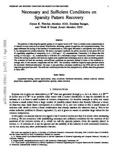
• b) there exists a general solution x = Ψ(α, p, t; c) with α ∈ Rn . Strategy of the proof: We split the proof in two parts. First, we prove that a) ⇒ b), that is, assuming the existence of real singularities for an open set of initial conditions, the leading behavior α must be real-valued. Second, we show that b) ⇒ a), that is the existence of general solutions with real leading behavior is enough to ensure the existence of finite time blow-up on an open set of initial conditions. The main idea is to use the local representation of the series (x = Ψ(α, p, t; c)) to build an open set of initial conditions. To do so, we show that there exists a homeomorphism M : C → X0 , between an open set of arbitrary constants C ⊂ Rn appearing in the general solutions and an open set of initial conditions X0 leading to finite time blow-up (see Fig 2). A. a) ⇒ b)

Let x0 ∈ X0 ⊂ Rn . By hypothesis, there exists a t∗ ∈ R which is the blow-up time associated with x0 . For all t ∈ ]t∗ − γ, t∗ [, x(t; x0 ) is real (since t is real). In this interval, we can use the representation of x(t; x0 ) provided by (8): 

x(t; x0 ) = Re(x) = τ p Re(α) +

∞ X

Re(aj ) τ

j=1

Im(α) +

∞ X

Im(aj ) τ q = 0,

j q

+ Im(α) +

∞ X

j=1

This implies that

j

j q



Im(aj ) τ  .

(15)

(16)

j=1

for all t ∈ ]t∗ − γ, t∗ [. This, however, implies that Im(α) = Im(aj ) = 0 ⇒ α ∈ Rn , 10

(17)

M

C

c3

c2

M

x3

X0

x2

-1

c1 = t

x1

*

The set of arbitrary constants augmented by t

The set of initial conditions leading blow-up at time t

*

*

FIG. 2. The map M maps an open set of arbitrary coefficient to an open set of initial conditions leading to finite time blow-up. B. a) ⇐ b)

By assumption, we can represent, locally around a movable singularity t∗ , a solution of x˙ = f (x), f ∈ Fn by a series of the form x = Ψ(α, p, t; c) where α ∈ Rn . According to Lemma 2, we have: c ∈ Rn , α ∈ Rn ⇒ Ψ(α, p, t; c) ∈ Rn ∀t ∈ ]t∗ − γ, t∗ [ .

(18)

¯ ⊂ Rn , and for all c ∈ C, the series Therefore, we can choose an open set C ⊂ C Ψ(α, p, t; c) can be used to define a set of initial condition leading to finite-time blow-up. Indeed for c ∈ C, we can pick t0 = t∗ − γ2 and define: x0 = Ψ(α, p, t0 ; c),

(19)

where (α, p) is a given balance corresponding to a general solution with α ∈ Rn . The solution x(t) based on the initial condition x0 will blow-up at t∗ = t0 + γ2 . By varying c in C, we can define the set X0 : ½

¾

γ X0 = x0 = Ψ(α, p, t0 ; c); c ∈ C, t0 = t∗ − . 2

(20)

In order to show that X0 is an open set, we have to prove that the map M M : C → X0 ,

(21)

is a homeomorphism. This in turn implies that M −1 is continuous and therefore that X0 = M −1 (C) is an open set. 11

Thus, choosing the set C to be real and open gives us that the set X0 of corresponding initial conditions is also real and open. We now prove that the map M is a homeomorphism, that is, it is (i) single-valued and one-to-one and (ii) continuous. (i) M is single-valued and one-to-one We consider two initial conditions x0 = x(t0 ; ck ), x˜0 = x(t0 ; c˜k ), ∈ X0 by considering c, c˜ ∈ C in such a way that ck 6= c˜k for k > 1 and ci = c˜i , i 6= k. Accordingly, we define x˜(t) = x(t; c˜k ). Then from the Psi-series (8), we have: ´

(22)

x0 = x˜0 ⇐⇒ x(t) = x˜(t) ⇐⇒ ck = c˜k ,

(23)

r

³

1

x(t) − x˜(t) = (ck − c˜k ) τ p+ q 1 + O(τ q ) , for all t0 ≤ t < t∗ , so that

where the first correspondence is a direct consequence of the existence and uniqueness of the solutions away from t = t∗ . Next, we consider the case where c˜1 6= c1 (that is t˜∗ 6= t∗ ). Let x˜0 = x(t0 ; c˜1 ) while x0 = x(t0 ; c1 ) with ci = c˜i , i > 1. Let x(t) = x(t; x0 ) be the solution based at x0 . The following equality follows from the fact that the Psi-series are functions of (t∗ − t) only: Ψ(α, p, t; (c1 , c2 , . . . , cn )) = Ψ(α, p, t + a; (c1 + a, c2 , . . . , cn ))

∀ a ∈C.

(24)

As a consequence, we have: x˜0 = Ψ(α, p, t0 ; c˜) = Ψ(α, p, t0 ; (t˜∗ , c2 , . . . , cn )) = Ψ(α, p, t0 + (t∗ − t˜∗ ); (t∗ , c2 , . . . , cn )) = Ψ(α, p, t0 + (t∗ − t˜∗ ); c)) = x(t0 + (t∗ − t˜∗ ); x0 ).

(25)

Therefore, by the uniqueness of the solutions, we have x0 = x˜0 if and only if t∗ = t˜∗ (the case where t∗ 6= t˜∗ and x0 = x˜0 can only happen on periodic orbits which are excluded here since all orbits blow-up in finite time). By the same token, due to to the continuity of the flow, the relation (25) guarantees that the map M is continuous in the variable c1 . (ii) M is continuous By definition, the map M is continuous if ∀ǫ > 0, ∃ ηǫ ∋ k c˜ − c k< ηǫ ⇒k X˜0 − X0 k< ǫ,

(26)

where c˜ ∈ C and k . k is the infinity norm. We have already shown that the map M is continuous with respect to its first argument (c1 ). Now, let 12

k c˜ − c k= |˜ ck − ck |,

(27)

for one or more of the ck (k > 1). Let β = γ2 , then by definition β = t∗ − t0 and 0 < β ≤ 21 . Since the series x0 = Ψ(α, p, t0 , c) and x˜0 = Ψ(α, p, t0 , c˜) converge, so does the series for x0 − x˜0 : x0 − x˜0 = (ck − c˜k )β p+rk +

∞ X

j

j=rk +1

(aj − a ˜j )β p+ q ,

(28)

where rk is the k-th resonance and cj = c˜j ∀ j < k. Since this series converges, the tail can be made arbitrarily small, i.e. for any finite pair of values ck and c˜k , we have ∀ν > 0, ∃ N(ck ,˜ck ) ∈ N ∋ |

∞ X

j=N(ck ,˜ck )

j

(aj − a ˜j )β p+ q | < ν.

(29)

Let N = sup {N(ck ,c˜k ) }. ck ,c˜k ∈C

From the polynomial recursion relations (13), it follows that aj = aj (ck ) is continuous (see appendix). Similarly, a ˜j is continuous in c˜k and so (aj − a ˜j ) is a continuous function of both ck and c˜k − ck . Therefore, for any fixed ck , the following is true: ∀µ > 0, ∃ ηj > 0 ∋ |˜ ck − ck | < ηj ⇒ |aj − a˜j | < µ for j < N. Let η =

inf

j∈{0,...,N −1}

ηj for a given µ. Choosing |c˜k − ck | < η guarantees that

|˜ x0 − x0 | ≤ |β p+rk Letting ν =

ǫ 2

(30)

N −1 X j=0

j

(˜ aj − aj )β q | + ν ≤ (µβ p+rk

∞ X

j=0

j

βq) + ν ≤ µ

β p+rk 1

1 − βq

+ ν.

(31)

1 q

and µ = ǫ 2β1−β p+rk , we obtain |˜ ck − ck | < η ⇒ |x˜0 − x0 | < ǫ.

Thus, the map M is continuous in ck for all k = 1, . . . , n.

(32) ⊓ ⊔

IV. SECONDARY RESULTS A. Absence of singularities and blow-up regions

As an obvious consequence of the theorem, the absence of real singularities can be tested: Corollary 1: The system x˙ = f (x), f ∈ Fn does not have finite time singularities if for all general solutions of the form (6), Im(α) 6= (0, . . . , 0). In general, the open set of initial conditions leading to a blow-up cannot be computed. However, the orthant in phase space (i.e. one of the 2n regions of Rn defined by {sign(xi ), i = 1, ..., n}) where blow-up occurs can be readily obtained: 13

Proposition 2: The orthant in phase space in which blow-up occurs is the orthant of α ∈ Rn . Proof 2: When blow-up occurs, the leading behavior is dominant, therefore, for t close enough to the singularity we have: 1

xi (t) = αi (t∗ − t)p + O((t∗ − t)p+ q ). Therefore the sign of xi is given by the sign of αi .

(33) ⊓ ⊔

Note here that the orthant is defined including the border axes (for instance in twodimensions (x1 , x2 ), the first quadrant {+, +} includes the semi-axes x1 ≥ 0 and x2 ≥ 0). This accounts for the case where some components of the p vector are positive. B. Finite time blow-up and first integrals

We now discuss the existence of finite time blow-up in the presence of first integrals. In some cases, polynomial systems x˙ = f (x) can have first integrals, that is function J = J(x, t) such that J˙ = ∇J.f + ∂t J = 0. These first integrals are constant on any solutions of the system. In some instances, these conserved quantities can be used to prove directly the absence of finite time blow-up. For instance, if a two-dimensional system has a first integral J = x21 + x22 , it is straightforward to see that there is no possibility of finite-time blow-up (J = x201 + x202 = x21 + x22 ∈ R ⇒ x1 , x2 ∈ R ∀ t). If, however, J = x21 − x22 , then blow-up cannot be ruled out as the solutions may go to infinity in such a way that the difference of the squares remains constant. It is therefore straightforward to prove that: Proposition 3: Let J = J(x, t) be a first integral for the system x˙ = f (x), x ∈ Rn . ∂J If the level sets of J are compact and ∂x 6= 0 ∀ i, then there is no finite time-blow-up. i ∂J 6= 0 ∀ i implies that there exist a first integrals on all variables. The condition ∂x i This condition is necessary to prevent blow-up in variables not contained in J. For instance the 4 dimensional system x¨ = x3 , y¨ = −y 3 has finite time blow-up (for an open set of initial conditions) despite the existence of the positive definite first integral J = (y) ˙ 2 + y 4 /4. How is this well-know result related to Corollary 1 on the absence of blow-up? If J = J(x, t) is a first integral for the system x˙ = f (x), then there exists a first integral b Jb = J(x) for the system x˙ = fb(x), where fb(x) is, as before, a dominant part of the vector field. That is, the system x˙ = fb(x) has an exact solution x = ατ p and f = fb + fˇ; b ˇ J(x, t) = (J(x) + J(x))g(t). In other words, the dominant part of the first integral is a first integral of the dominant part of the vector field (See [8] for further details). Since the first integral Jb is constant on all solutions, it is constant on the particular solution p d b b b x = ατ p , therefore J(ατ ) = J(α)τ = 0 ⇒ J(α) = 0. However, if J(x, t) is of definite b b sign, so is J(x, t) and therefore the relation J(α) = 0 cannot be satisfied if α ∈ Rn , which proves that Proposition 3 is a direct consequence of Corollary 1. So, the fact that

14

Jb is of definite sign implies that the corresponding balance (α, p) is such that Im(α) 6= 0. Moreover, we can propose an upgraded version of Proposition 3: b Proposition 3’: Let Jb = J(x) be a first integral of a dominant part of the system n ∂ Jb 6= 0 ∀ i, then there is no x˙ = f (x), x ∈ R . If the level sets of Jb are compact and ∂x i finite time-blow-up.

See Section V.B for an illustration of Proposition 3’. V. APPLICATIONS A. A simple example

We consider the system x˙ 1 = x1 (a + bx2 ), x˙ 2 = cx21 + dx2 ,

(34.a) (34.b)

with b > 0, c > 0. This system arises from the reduction of a semilinear parabolic PDE [1]. The existence of finite time blow-up for this system is used to prove the finite time blow-up of the PDE. We show how our theorem can be used to immediately determine the existence of finite time blow-up for this system. The first step of the analysis is to determine the different balances, that is the different possible dominant truncations of the vector field. In this case, we find two balances both corresponding to the truncation: f=

Ã

x1 (a + bx2 ) cx21 + dx2

!

,

fb =

Ã

bx1 x2 cx21

!

,

fˇ =

Ã

ax1 dx2

!

,

(35)

and p = (−1, −1). That is, the system x˙ = fb(x) has two exact solutions of the form x = ατ p with α = ( √±1bc , 1c ). It is easy to check, using (12), that the resonances are, in both cases, r = −1 and r = 2. These two balances define Psi-series solutions where logarithmic terms enter as coefficients of the term τ p+r = τ 1 . Therefore, we can apply our main theorem and state that for all b, c such that bc > 0 the system (34) exhibits finite time blow-up, that is there exist open sets of initial conditions in R2 such that all solutions based on this set blow-up in finite-time. Moreover, the blow-up occurs both in the first ({+, +}) and fourth ({−, +}) quadrants (see Proposition 2). B. Absence of finite-time singularity for the Lorenz system

The Lorenz system is ubiquitous in dynamical system theory [31,32] integrability theories [33,34] and singularity analysis theory [35,36,8]. The boundedness of its solution was proved in [10]. The system reads:

15

x˙ = σ(y − x) y˙ = ρx − y − xz z˙ = xy − βz,

(36.a) (36.b) (36.c)

where x, y, z, σ, β, ρ ∈ R. The Lorenz system has only two balances characterized by the leading behavior p = (−1, −2, −2) and α = (±2i, ∓2i/σ, −2/σ). Both balances are associated with the truncation: 



σy  b f =  xz  , xy





σx  ˇ f =  ρx − y  , −βz

(37)

These balances define the first terms of the Psi-series characterizing the local solutions around the singularities. The resonances are Spec(R) = {−1, 2, 4} which shows that the Psi-series are the general solutions around the singularities. Moreover, it has been proved that the Psi-series are convergent [29]. Therefore, it follows from the main theorem that the solutions of the Lorenz system never exhibit finite-time blow-up in the variable x. Let us also note that the dominant truncation of the vector field fb has two first integrals Jb1 = y 2 + z 2 and Jb2 = x2 − 2σz. From proposition 3’ and the definiteness of Jb1 , it follows that the variables y, z never blow up. However, as already stressed, this is not enough to rule out finite time blow-up in the variable x. C. Fluid Dynamics example

In order to model the interaction between vorticity and shear in turbulent flow [14], Vieillefosse introduced a five dimensional ODE system whose blow-up shows that the flow of an incompressible and inviscid fluid diverges in a finite time. The existence of finite time blow-up is proven by decoupling the system and reducing the dynamics of one of its variables to a Hamiltonian dynamic with a simple potential. We show here how this result can be obtained in a straightforward way. The system reads (in our notation): x˙1 = −(x3 + x4 ) x˙2 = x4 1 1 3 x˙3 = − x5 + x1 x2 − x21 2 2 4 1 1 2 1 x˙4 = x5 + x1 x2 − x2 2 6 3 1 2 x˙5 = x4 x1 − x2 x4 3 3

(38.a) (38.b) (38.c) (38.d) (38.e)

We find that there is a balance (α, p) characterized by the leading exponents p with leading order coefficients α: p = (−2, −2, −3, −3, −4) α = (144, 72, −432, 144, 864) 16

(39.a) (39.b)

Since the leading order coefficients are real, the general solution of this system will exhibit finite-time blow-up if the balance we have chosen indeed corresponds to a general solution. Checking, we find that the resonances are r = 2, r = 3, r = 4 and r = 6. Therefore, there exists a general Psi-series solution based on this balance. As a consequence of the main theorem, the general solution will exhibit finite time blow-up for some open set of real initial conditions. Moreover, the blow-up occurs on the orthant {+, +, −, +, +} (see Proposition 2). D. MHD example

In all the examples so far, the existence (or absence) of finite time blow-up was already know using specific methods. We now apply our results to a physical system where blow-up is only known to occur numerically but for which the existence of blow-up has never been rigorously demonstrated. The system in question, introduced by Klapper, Rado, and Tabor [16], models ideal three-dimensional incompressible magnetohydrodynamics. The trace equations for such a system near magnetic null points are defined as follows: h

Tn = Trace (∇u)n h

i

Pn,m = Trace (∇u)n (∇b)m

(40.a) i

(40.b)

where u = the fluid velocity field and b = the magnetic field. It is believed that the blow-up of this system in finite time could explain certain large solar flares and solar dynamos. We now prove the existence of finite time singularities using our theorem. The model written in the variables (x1 , x2 , x3 , x4 , x5 , x6 ) ≡ (T2 , T3 , P1,2 , P2,2 , P1,1 , P2,1 ) reads x˙1 = −2x2 + 2x3 1 x˙2 = − x21 − βx1 + 3x4 2 1 2 β x˙3 = β + x1 − x4 6 3 1 1 2 2 x˙4 = − x1 x3 + βx3 − βx2 + γx5 3 3 3 3 x˙4 = γ − x6 1 1 x˙6 = − x1 x5 + βx5 3 3

(41.a) (41.b) (41.c) (41.d) (41.e) (41.f)

There are several possible balances. However, only one gives a full set of non-negative rational resonances. We find by checking the eigenvalues of R (see 12) that the resonances are {−1, 0, 0, 3, 3, 6} for the following balance: p = (−2, −3, −1, −2, −1, −2) α = (6, −6, α3 , 2β − α3 , α5 , −α5 ) 17

(42.a) (42.b)

The arbitrariness of the leading terms α3 , α5 reflects the fact that r = 0 is a resonance with multiplicity two. This is then a balance that yields a general local solution of the form (8). Note that the leading order coefficients are real, or can be chosen real for the proper initial data. Thus, our theorem predicts that there is an open set of real initial conditions (which make α3 and α5 real) for which the general solution to this system blows up in finite time. Interestingly enough, our result can also be used to give an estimate of the blow-up time. Indeed, close to the singularity the dynamic is controlled by the most dominant part of the vector field (the truncation fb of the vector field associated with the given balance). For the system x˙ = fb(x), the two first equations decouple leading to a simple closed system x¨1 = x21

(43)

Therefore, if the system is close enough to the singularity, the blow-up time can be predicted by integrating this system. That is, if for a given time t1 we know the values of x1 (t1 ), x˙ 1 (t1 ), then t∗ = t1 + √

Z x1 (t) 1 dx1 r lim 2E1 t→∞ x1 (t1 ) x3 1 + 3E11

(44)

where E1 = 12 x˙ 1 (t1 )2 − 31 x1 (t1 )3 . This last integral can be expressed in terms of an elliptic integral of the first kind: √ 12 5Π 3 F (α, sin t∗ = t1 + √ ) (45) 6 12 8E1 −1

³

√ ´ 1−√3−x1 (t1 ) . 1+ 3−x1 (t1 )

where α = cos In order to get close to the singularity, we can start with an initial condition x0 = x(0) and compute the value x(t1 ) by expanding the solutions in Taylor series up to a given order N : x(t) =

N X

ai ti + O(tN +1 )

(46)

i=0

where a0 = x0 and the values of the coefficients ai as functions of x0 can be found by inserting the Taylor series in the system x˙ = f (x) and equating power by power. This Taylor series has a finite radius of convergence tmax which can be found by studying the Taylor approximations as N increases. We can now choose t1 < tmax and find the value of x(t1 ). These values are then used to compute the blow-up time t∗ through an estimate like (45). This method is not a general method since it is not guaranteed that tmax will be in the radius of convergence of the Psi-series (indeed tmax could be constrained by complex rather than real singularities). However, further approximations of the solutions can be obtained by analytic continuation and/or Pad´e approximants. For the system studied here this method provides an excellent approximation of the blow-up time. As an example, we choose the following initial conditions leading to blowup: x0 = (−20, −10, −20, 178/3, 5, 24) and γ = 20, β = 4. Using successive Taylor 18

approximations with N ≤ 25 we find that tmax ≈ 0.55. Picking t1 = 0.5, we obtain x1 (t1 ) ≈ −4.78, x˙ 1 (t1 ) ≈ 59.23 and t∗ ≈ 1.50, to be compared with the numerical value t∗,num = 1.54 obtained by using the dedicated ATOMFT package [37]. VI. CONCLUSIONS

We have found necessary and sufficient conditions for finite time singularities for a large class of ODEs. These conditions rely on the analysis of the local series solutions around the singularities and can be expressed as a reality condition on the leading behavior of the solutions near blow-up. Roughly speaking, finite time blow-up will occur if and only if the dominant terms in the local general series are real. In order to find which series correspond to the general solution (among the plethora of local solutions) we investigated the resonances and the corresponding arbitrary coefficients of the Psi-series. This allowed us to find a homeomorphism between an an open set of initial conditions and open set of arbitrary constants. Moreover, we were also able to determine the location in phase-space where blow-up occurs and explore the relationship between the absence of finite time singularities and first integrals. To illustrate these different results we analyzed different examples from different fields of applied mathematics. The class of systems considered here was constrained by the requirement that the Psiseries exist. As we already stated, this encompasses a large class of systems. However, we believe that this limitation is merely technical. Indeed, the results do not rely on the specific form of the Psi-series but only on the fact that they describe general solutions. The reality condition applies only to the most dominant terms near blow-up. Therefore, we conjecture that our main theorem is actually valid for a much larger class of systems and that the conditions on the leading exponents and resonances (as being rational numbers) could be relaxed to the case where they are real numbers. If this conjecture holds, it could provide a universal way of detecting the existence of blow-up for systems of ordinary differential equations. Another limitation of our results is the fact that we considered, for the sake of simplicity, only general solutions of ODEs rather than singular solutions. This point was important in establishing the existence of the homeomorphism between initial conditions and arbitrary coefficients. However, our results could probably be extended by considering the possibility of blow-up for singular solutions. Indeed, some systems may exhibit finite-time blow-up only for constrained sets of initial conditions rather than open sets. The solutions based on these sets are not in the set of general solutions, however their asymptotic behavior near blow-up can still be analyzed by studying the balances (α, p) corresponding to singular solutions (that is the Psi-series with less than n − 1 arbitrary coefficients). Similar results on the blow-up of singular solutions could then be obtained. An interesting consequence of our main theorem is that the blow-up of a system ultimately depends only on the dominant behavior, that is the balance (α, p). These balances are computed from the knowledge of the dominant part of the vector field (in the case that the vector field is homogeneous, the dominant part is, roughly speaking, given by the terms of maximal degree only). Therefore, we see that the blow-up is controlled only by these terms and not by lower order terms (such as the linear terms 19

for instance). The effect of the lower-order terms could be to create regions in phasespace where the solutions are bounded but they never manage to prevent the solution to blow-up in the entire phase-space. This point is important because in many instances the dominant part of a given vector field assumes a simple form and can be exactly integrated (by quadratures or by showing explicitly the existence of a set of first integrals). In turn, these explicit solutions can be used to compute an estimate of the blow-up time as a function of the initial conditions. This estimate becomes better as one approaches the blow-up point. It is well-known that near fixed points the solutions of a given system of ODEs essentially behave according to the linear part, and most of the subsequent dynamical analysis rely on perturbation expansions around the linear solutions (the normal form theory `a la Poincar´e-Dulac is based on this basic idea). The theory developed in this paper shows that the most nonlinear part of the vector field determines the behavior of the solutions near its singularities. We believe that a thorough understanding of the dynamics of unbounded systems can only be achieved by merging the two approaches and we hope that the ideas presented in this paper may provide a first step in this direction. VII. APPENDIX

We now prove Lemmas 1 and 2: Lemma 1: The series given in (8) is a general formal solution to the system (6). Lemma 2: Let x = Ψ(α, p, t; c2 , . . . , cm ) be a solution of x˙ = f (x) around the singularity t∗ containing (m − 1) arbitrary coefficients. If α ∈ Rn , and ci ∈ R ∀ i = 2, . . . , m then, ajk ∈ Rn ∀ (j, k) Proof of Lemmas 1 and 2: In order to prove these lemmas, we first look at the form of the recursion relations. We begin by writing an expression for the ith component of the n-dimensional equation (9), i.e. x˙i = fi (x) = fbi (x) + fˇi (x)

(47)

We also rewrite the Psi-series (8) for a single component of x: pi

xi = τ (

Nj ∞ X X

(i)

j

aj,k τ q (log τ )k )

(48)

j=0 k=0

where τ = (t∗ − t) and a0,0 = α. The aj,k coefficients are now constants. In order to obtain a generic recursion relation, it is necessary to introduce a specific form for fbi and fˇi . Thus, let Mn 1 M2 fbi (x) = a xM 1 x2 · · · xn mn 1 m2 fˇi (x) = b xm 1 x2 · · · xn

20

(49.a) (49.b)

Without loss of generality, we have made both fbi and fˇi consist of only one polynomial term, but it will hopefully be apparent to the reader that the general form of the recursion relations which result from this would be unchanged for an arbitrary number of terms. Since fbi (x) is the dominant balance term, it will by definition have a leading-order power of τ which matches that of x˙i (i.e. it will go as τ pi −1 ), while the leading order term j of fˇi (x) will be at least one order higher (so that it goes as τ pi −1+ q or higher). Thus, equation (47) becomes −τ

pi −1

·X

¸

X j (i) j (i) j ( + pi )aj,k τ q (log τ )k + k aj,k τ q (log τ )k−1 = j=0 q j=0

k=0

aτ

pi −1

· X

(

k=0

(1) aj,k τ

j q

k M1

(log τ ) )

1

· X

(2) aj,k τ

j q

k M2

(log τ ) )

j=0 k=0

j=0 k=0

b τ pi −1+ q (

(

X

(1)

j

aj,k τ q (log τ )k )m1 (

j=0 k=0

X j=0 k=0

(2)

···(

X

(n) aj,k τ

j q

k Mn

(log τ ) )

j=0 k=0

j

aj,k τ q (log τ )k )m2 · · · (

X

(n)

j

¸

+

aj,k τ q (log τ )k )mn

j=0 k=0

¸

J

If we now consider collecting terms of order τ q +pi −1 , it is clear that these will only involve coefficients whose first index is less than J (i.e. aj,k with j < J) except in the case where there is a product of a single aJ,k times many a0,0 . Furthermore, this last case will only occur for the dominant balance term, as the highest j value for an aj,k appearing at this order in the fˇi term would be j = J − 1. We therefore deduce that the J recursion relation for the ith component of (9) at order τ q +pi −1 (log τ )K (valid only for J ≥ 1) is: −

³J

q

´

(i)

(i)

+ pi aJ,K − (K + 1) aJ,K+1 = (1)

(1)

(2)

(2)

(1)

(2)

(n)

(1)

(2)

(3)

(n)

(3)

(n)

M1 aJ,K (a0,0 )M1 −1 (a0,0 )M2 (a0,0 )M3 · · · (a0,0 )Mn +

M2 aJ,K (a0,0 )M1 (a0,0 )M2 −1 (a0,0 )M3 · · · (a0,0 )Mn + ··· +

(n)

(3)

(i)

Mn aJ,K (a0,0 )M1 (a0,0 )M2 (a0,0 )M3 · · · (a0,0 )Mn −1 + bJ,K (aj,k ; j < J)

(51.a)

which simplifies to −

³J

q

´

(i)

(i)

+ pi aJ,K = (K + 1) aJ,K+1 +

n ³ b X ∂ fi (a0,0 )

m=1

∂xm

(m)

´

(i)

aJ,K + bJ,K (aj,k ; j < J)

(52)

(i)

The bJ,K term is some undetermined polynomial of various aj,k coefficients for which j < J and k ≤ K. Equation (52) holds for any component i of the system, so upon dropping the index i and going back to the n-dimensional system, we get a matrix equation for the recursion relations: J (53) [−Dfb(a0,0 ) − I − diag(p)]aJ,K = (K + 1)aJ,K+1 + bJ,K (aj,k ; j < J, k ≤ K) q where Dfb(a0,0 ) is just the Jacobian matrix of fb evaluated at x = a0,0 (i.e. each xi is (i) evaluated at a0,0 ). Defining the matrix R ≡ [−Dfb(a0,0 ) − diag(p)] and dropping the capital indices, we shorten our notation to 21

(50.a)

j [R − I]aj,k = (k + 1)aj,k+1 + bj,k q

(54)

This is just an n-dimensional linear system with constant coefficients. It always has a unique solution except when qj is an eigenvalue of the matrix R. As discussed previously, these eigenvalues are the resonances, and we can see now why they correspond to arbitrary coefficients. One such resonance is always −1. Proof of Lemma 1: We only need to show that (54) does in fact have a solution. Since we are assuming that our Psi-series expansion represents a general solution to the system, there must be n − 1 non-negative rational resonances, not necessarily distinct (note that q is the l.c.d. of these resonances). For now, we will deal with the case where for every repeated eigenvalue, its algebraic multiplicity will equal its geometric multiplicity (i.e. the number of orthogonal eigenvectors associated with it will equal its multiplicity) so that the total number of arbitrary parameters contained in all the eigenvectors will still be n − 1. Let rqm denote the mth non-negative resonance. As long as j < r1 , aj,k will be zero except when k = 0. Let us write the recursion relations at k = 0 in the following form: Rj aj,0 = aj,1 + bj,0

(55)

where here and throughout the remainder of the appendix, we define Rj ≡ R− qj I. When 0 < j < r1 , the matrix Rj is invertible, so a solution exists for any aj,1 and all bj,0 . Recall that the a0,0 coefficients are determined by balancing the leading order terms and, by assumption, there is no need for a logarithm at leading order. Therefore b1,k = 0 for all k ≥ 1. But then the recursion relations at j = 1 and k ≥ 1 will be R1 a1,k = (k + 1)a1,k+1 ,

(56)

so that, in order to avoid an infinite chain of linear equations, we must set a1,k = 0 for all k ≥ 1. But then b2,k = 0 for all k ≥ 1, so by the same argument a2,k = 0 for all k ≥ 1. This process continues as we increase j so long as j < r1 , i.e. so long as Rj is invertible, and thus aj,k = 0 for all k ≥ 1 whenever j < r1 . The introduction of the first logarithm may occur at j = r1 if the recursion relation for ar1 ,0 fails to satisfy the solvability condition for the non-invertible matrix Rr1 . (In the case that r1 = 0, there would be no logarithm until r2 . Having r1 = 0 simply means that some of the components of a0,0 are arbitrary. For this discussion, we will assume r1 > 0.) It is possible that br1 ,0 will not lie in the range of the matrix Rr1 . Let yr1 denote a normalized null vector of Rr1 (assume for now that there is only one). Since we are currently operating under the assumption that the matrix R has a full set of eigenvectors, there will be no generalized eigenvectors at all, and thus the null vector(s) of Rrm will never lie in the range of Rrm . We can therefore solve Rr1 ar1 ,0 = ar1 ,1 + br1 ,0

(57)

even in the case where br1 ,0 is not in the range of Rr1 by looking at the recursion relation at k = 1: 22

Rr1 ar1 ,1 = 0

(58)

while still setting ar1 ,k = 0 whenever k ≥ 2. The solution of (58) is ar1 ,1 = cyr1 , where c is an arbitrary constant. The solvability condition for (57) will now be c < v|yr1 > + < v|br1 ,0 >= 0

(59)

where v is the null vector of the adjoint of Rr1 and < | > denotes the inner product. This condition is automatically satisfied by choosing the heretofore arbitrary c to be c=−

< v|br1 ,0 > . < v|yr1 >

(60)

Since yr1 does not lie in the range of Rr1 , the denominator of this expression will be non-zero. Thus, we have regained solvability by introducing one power of log τ at this order. Note that we still a retain an arbitrary parameter, as the solution to (57) will be a particular solution plus c˜yr1 where c˜ is arbitrary. The reader can check that the same procedure works in the case where Rr1 has multiple orthogonal null vectors, with the number of arbitrary parameters retained equal to the number of null vectors. For j > r1 , the log τ introduced at j = r1 may be raised to various powers for higher j values due to the non-linearities (of degree up to M ) in the bj,k terms . Thus, when r1 < j < r2 , higher and higher powers of log τ may build up so that bj,k 6= 0 for higher and higher values of k. However, as long as Rj is invertible, solutions for the coefficients will still exist. Let n ˜ j,k ≡ sup {n|rk ≤ nrj }. n∈Z+

(61)

Then for j = r2 , the highest possible power of log τ in the recursion relations will be (log τ )n˜ 2,1 , i.e. the highest value of k for which br2 ,k 6= 0 will be n ˜ 2,1 ≡ n ˜ . As before, we propose only one power of log τ beyond this, so that we get the following system of recursion relations: Rr2 ar2 ,˜n+1 = 0 n + 1)ar2 ,˜n+1 + br2 ,˜n Rr2 ar2 ,˜n = (˜ n)ar2 ,˜n + br2 ,˜n−1 Rr2 ar2 ,˜n−1 = (˜ .. . Rr2 ar2 ,1 = 2ar2 ,2 + br2 ,1 Rr2 ar2 ,0 = ar2 ,1 + br2 ,0

(62.a) (62.b) (62.c) (62.d) (62.e)

Let yr2 be the only null vector of Rr2 and v the null vector of the adjoint Rr∗2 . Then the solution of (62.a) is ar2 ,˜n+1 = c1 yr2 with c1 arbitrary. This can be used to satisfy the solvability condition of (62.b) by choosing c1 = −

< v|br2 ,˜n > . (˜ n + 1) < v|yr2 > 23

(63)

The solution of (62.b) will then be ar2 ,˜n = c2 yr2 + xp , where xp is the particular solution and c2 is arbitrary. This can then be used to satisfy the solvability condition for (62.c) by demanding c2 =

−(< v|br2 ,˜n−1 > +˜ n < v|xp >) (˜ n) < v|yr2 >

(64)

and so on, so that all of the solvability conditions are met and we still have one arbitrary constant from ar2 ,0 . In general, we can predict the highest power of log τ appearing in the recursion relations at j = rm (i.e. the highest k for which brm ,k 6= 0) by looking at the values of n ˜ rm ,i for i < rm . Then, if the solvability conditions are not satisfied at this power of log τ , we must add at most one more power of log τ , assuming there are a complete set of eigenvectors. Thus, at j = r3 , the highest possible logarithmic power will be given by (log τ )Nr3 , where Nr3 = sup{˜ n3,1 + 1, (˜ n2,1 + 1)˜ n3,2 + 1},

(65)

˜ ≡ supj,k {˜ and so on. For brevity, if we let N nj,k }, then a strict upper bound for the power of log τ at order j = rm is given by Bm , where ˜ m−1 + N ˜ m−2 + · · · + N ˜ +1 Bm = N

(66)

At any value of j in the recursion relations, the highest power of log τ will always be bounded by some finite integer Nj , but Nj → ∞ as j → ∞. Let us now consider the case in which one of the positive eigenvalues rqm of the matrix R has a multiplicity exceeding the number of eigenvalues that go with it. Assume there is only one eigenvector. Then the algebraic multiplicity of rqm is equal to the number of generalized eigenvectors (including the actual eigenvector) associated with the eigenvalue rm . (In general, a chain of generalized eigenvectors can begin with every eigenvector if q there is excess eigenvalue multiplicity.) Without loss of generality, let us assume an eigenvalue multiplicity of 3 with only one eigenvector. Using the variable yrm to denote the eigenvector (which is also the null vector of Rrm ), we have the following relationships for the generalized eigenvectors: Rrm y r m = 0 Rrm z0 = yrm Rrm z1 = z0

(67.a) (67.b) (67.c)

The vectors z0 and z1 are the generalized eigenvectors associated with yrm . All three of these vectors can be chosen orthonormal, and we will assume that this has been done here. It is a fact that, for the eigenvalue multiplicity of 3, there can be no more generalized eigenvalues than these. Thus, z1 is not in the range of the matrix Rrm , but both yrm and z0 are. Once again, we let v be the null vector of Rr∗m , and we will let κ be the highest value of k for which bj,k 6= 0. Then the recursion relation at k = κ is: Rrm arm ,κ = (κ + 1)arm ,κ+1 + brm ,κ 24

(68)

Since yrm is now in the range of Rrm , we cannot guarantee that this equation is solvable merely by letting arm ,κ+1 = cyrm with c arbitrary. If we were to attempt this, then letting v be the nullvector of Rr∗m as before, the Fredholm condition on the right hand side of (68) would be < v|(κ + 1)c yrm > + < v|brm ,κ >=< v|brm ,κ >≡ 0

(69)

which may not be satisfied by brm ,κ . Thus, instead of adding one power of log τ at k = κ + 1, we add three powers, giving the following additional recursion relations: Rrm arm ,κ+3 = 0 Rrm arm ,κ+2 = (κ + 3)arm ,κ+3 Rrm arm ,κ+1 = (κ + 2)arm ,κ+2 .

(70.a) (70.b) (70.c)

The solutions to these are clearly arm ,κ+3 = c0 yrm arm ,κ+2 = c1 yrm + c0 (κ + 3)z0 arm ,κ+1 = c2 yrm + c1 (κ + 2)z0 + c0 (κ + 2)(κ + 3)z1

(71.a) (71.b) (71.c)

where c0 , c1 , and c2 are all arbitrary. Substituting (71.c) into (68) gives Rrm arm ,κ = (κ + 1)c2 yrm + c1 (κ + 1)(κ + 2)z0 + c0 (κ + 1)(κ + 2)(κ + 3)z1 + brm ,κ . (72) We know from our previous discussion of the generalized eigenvectors that both < v|yrm >= 0 and < v|z0 >= 0, but < v|z1 >6= 0. Thus, applying the Fredholm solvability condition to the right hand side of (72) gives c0 (κ + 1)(κ + 2)(κ + 3) < v|z1 > + < v|brm ,κ >≡ 0,

(73)

so that by choosing c0 = −

< v|brm ,κ > (κ + 1)(κ + 2)(κ + 3) < v|z1 >

(74)

the recursion relation (72) becomes solvable. Note that now the solution of (72) becomes arm ,κ = c3 yrm + c2 (κ + 1)z0 + c1 (κ + 1)(κ + 2)z1

(75)

so that a proper choice of c1 will satisfy the solvability condition of the recursion relation for arm ,κ−1 , and so on. Three arbitrary parameters will be kept by the solution for arm ,0 , so that we still get a full set of arbitrary parameters equal to the multiplicity of the eigenvalue rqm . In general, if we let β equals the number of generalized eigenvectors (including the actual eigenvector) in the largest “chain” of generalized eigenvectors, then the maximum power of log τ at j = rm will be given by (log τ )κ+β with κ as defined above. Thus we see that for the class of systems we are dealing with (those that have rational leading order exponents and rational eigenvalues for the R matrix), a solution to the 25

recursion relations derived from the Psi-series expansion (8) always exists with the proper number of arbitrary parameters, simply by adding a limited number of powers of log τ at each resonance. This proves Lemma 1. ⊓ ⊔ Proof of Lemma 2: We are given that the leading order coefficients α, which we now call a0,0 , are real. The recursion relation (54) is a simple linear system, and for the class of systems we are considering , q and diag(P ) are real. Therefore, the matrix R appearing in (54) is real. It is a fact that solutions to linear systems with real coefficients and real inhomogeneities are themselves real, so a0,0 ∈ Rn ⇒ b1,k ∈ Rn ∀k ⇒ a1,k ∈ Rn ∀k

(76)

as long as 1 < r1 , where it is to be understood throughout this proof that the only allowable values for k and j are non-negative integers. (Recall that, by assumption, a0,k = 0 for all k ≥ 1.) If r1 = 1, the solutions a1,k still consist of real values but with arbitrary coefficients which, by hypothesis, we choose to be real. In general, aj,k ∈ Rn ∀k ⇒ bj,k ∈ Rn ∀k ⇒ aj+1,k ∈ Rn ∀k

(77)

is not a resonance. Thus we can say that, for all j < r1 and all non-negative as long as j+1 q integers k, aj,k ∈ Rn . This implies that br1 ,k ∈ Rn for all k, so that the singular linear system for ar1 ,k consists of only real valued coefficients. This means that the solutions ar1 ,k will be real but with arbitrary coefficients. Since, by hypothesis, we choose all arbitrary coefficients to be real, ar1 ,k will be real for all k. This will be true at any resonance rqm for which aj,k is real for all j < rm and for all k. Thus we have that aj,k ∈ Rn ∀k ⇒ bj,k ∈ Rn ∀k ⇒ aj+1,k ∈ Rn ∀k

(78)

is a resonance, since, by hypothesis, we always choose the arbitrary even when j+1 q coefficients to be real. Therefore a0,0 ∈ Rn ⇒ aj,k ∈ Rn ∀j, ∀k. This proves Lemma 2.

(79) ⊓ ⊔

Acknowledgments This work is supported by DOE grant DE-FG03-93-ER25174. The authors would like to thank Michael Tabor for many stimulating interactions and Hermann Flaschka for interesting discussions on Liouville integrability. The authors are also indebted to Isaac Klapper and Anita Rado for providing them with the MHD example which served as a motivation for this work.

26

REFERENCES [1] B. Palais. Blowup for nonlinear equations using a comparison principle in Fourier space. Communic. Pure and Appl. Math., 41:165–196, 1988. [2] L. Glangetas and F. Merle. Existence of self-similar blow-up solutions for Zakharov equation in dimension two. part I. Commu. Math. Phys., 160:173–215, 1994. [3] M. Ohta. Blow-up solutions and strong instability of standing waves for the generalized Davey-Stewartson system in R2 . Ann. Inst. Henri Poincar´e, 63:111–117, 1995. [4] I. Peral and J. L. Vazquez. On the stability or instability of the singular solution of the semilinear heat equation with exponential reaction term. Arc. Rational Mech. Anal., 129:201–224, 1995. [5] Y. Matsumo. Two-dimensional dynamical system associated with Abel’s nonlinear diffrential equation. J. Math. Phys., 33:412–421, 1992. [6] M. J. Ablowitz, A. Ramani, and H. Segur. A connection between nonlinear evolution equations and ordinary differential equations of P-type I. J. Math. Phys., 21:715–721, 1980. [7] J. Weiss, M. Tabor, and G. Carnevale. The Painlev´e property for partial differential equations. J. Math. Phys., 24:522–526, 1983. [8] A. Goriely. Integrability, partial integrability and nonintegrability for systems of ordinary differential equations. J. Math. Phys., 37:1871–1893, 1996. [9] A. Goriely and M. Tabor. The singularity analysis for nearly integrable systems: homoclinic intersections and local multivaluedness. Physica D, 85:93–125, 1995. [10] B. A. Coomes. The Lorenz system does not have a polynomial flow. J. Diff. Eq., 82:386–407, 1989. [11] Marsden and Ratiu. Classical Mechanics. Springer Verlag, New York, 1994. [12] L. M. Hocking, K. Stewartson, and J. Stuart. A nonlinear instability burst in plane parallel flow. J. Fluid. Mech., 51:705–753, 1972. [13] U. Frisch and R. Morf. Intermittency in nonlinear dynamics and singularities at complex time. Phys. Rev. A, 23:2673–2705, 1981. [14] P. Vieillefosse. Local interaction between vorticity and shear in a perfect incompressible fluid. J. Physique, 43:837–842, 1982. [15] K. Ohkitani. Lagrangian frozen-in hypothesis for vortex stretching. J. Phys. Soc. Jpn, 62:390–394, 1993. [16] I. Klapper, A. Rado, and M. Tabor. A Lagrangian study of dynamics and singularity formation at magnetic null points in ideal three dimensional magnetohydrodynamics. Phys. Plasmas, 3:4281–4283, 1996. [17] A. M. Stuart and M. S. Floater. On the computation of blow-up. Eurto. Jnl of Applied Mathematics, 1:47–71, 1990. [18] A. Ramani, B. Grammaticos, and T. Bountis. The Painlev´e property and singularity analysis of integrable and non-integrable systems. Physics Reports, 180:159–245, 1989. [19] J. D. Fournier, G. Levine, and M. Tabor. Singularity clustering in the duffing oscillator. J. Phys. A, 21:33–54, 1988. [20] M. Tabor. Chaos and integrability in nonlinear dynamics. An introduction. Wiley Interscience, New York, 1989. 27

[21] A. Goriely. Investigation of Painlev´e property under time singularities transformations. J. Math. Phys., 33 (8):2728–2742, 1992. [22] M. Adler and P. van Moerbeke. The complex geometry of the Kowalewski-Painlev´e analysis. Invent. math., 97:3–51, 1989. [23] L. Brenig and A. Goriely. Painlev´e analysis and normal forms. In E. Tournier, editor, Computer algebra and differential equations, pages 211–238. Cambridge University Press, Cambridge, 1994. [24] S. Kichenassamy and W. Littman. Blow-up surfaces for nonlinear wave equations, I. Comm. PDE, 18:431–452, 1993. [25] S. Kichenassamy and W. Littman. Blow-up surfaces for nonlinear wave equations, II. Comm. PDE, 18:1869–1899, 1993. [26] S. Kichenassamy and G. K. Srinivasan. The structure of the WTC expansions and applications. J. Phys. A, 28:1977–2004, 1995. [27] P. L. Sachdev and S. Ramanan. Integrability and singularity structure of predatorprey system. J. Math. Phys., 34:4025–4044, 1993. [28] M. A. Hemmi and S. Melkonian. Convergence of Psi-series solutions of nonlinear ordinary differential equations. Canad. Appl. Math. Quart., 3:43–88, 1995. [29] S. Melkonian and A. Zypchen. Convergence of Psi-series solutions of the Duffing equation and the Lorenz system. Nonlinearity, 8:1143–1157, 1995. [30] S. Abenda. Asymptotic analysis of time singularities for a class of time-dependent Hamiltonians. J. Phys A, 30:143–171, 1997. [31] E. N. Lorenz. Deterministic nonperiodic flow. J. Atmospheric Sci., 20:130–141, 1963. [32] C. Sparrow. The Lorenz equations. Springer-Verlag, New York, 1982. [33] M. K´ us. Integrals of motion for the Lorenz system. J. Phys. A, 16:L689–L691, 1983. [34] H. J. Giacomini, C. E. Repetto, and O. P. Zandron. Integrals of motion for threedimensional non-Hamiltonian dynamical systems. J. Phys. A, 24:4567–4574, 1991. [35] H. Segur. Soliton and the inverse scattering transform. In A. R. Osborne and P. Malanotte Rizzoli, editors, Topics in ocean physics, pages 235–277. North-Holland publishing, Amsterdam, 1982. [36] G. Levine and M. Tabor. Integrating the nonintegrable: Analytic structure of the Lorenz system revisited. Physica D, 33:189–210, 1988. [37] Y. F. Chang and G. Corliss. Ratio-like and recurrence relation tests for convergence of series. J. Int. Math. App., 25:349–359, 1980.

28