437
Vol. 52, n. 2 : pp. 437-448, March-April 2009 ISSN 1516-8913 Printed in Brazil
BRAZILIAN ARCHIVES OF BIOLOGY AND TECHNOLOGY A N
I N T E R N A T I O N A L
J O U R N A L
Necessary Auxiliary Background for Efficient Use of an Existing Computer Program of Non-parametric Fitting of Nonlinear Equations Emmanuel M. Papamichael* and Leonidas G. Theodorou Sector of Organic Chemistry and Biochemistry; Laboratory of Enzymology; Department Chemistry; University of Ioannina 45110, Ioannina - GREECE
ABSTRACT This work constituted a significant contribution for more efficient use of a valuable computer program of nonparametric fitting of nonlinear multiparametric equations to experimental data. However, prerequisite in this context was the transformation of nonlinear multiparametric equations into linear hyperplane forms before their incorporation within the computer program; this latter was decisive and a matter of proper programming practice. Herein, a series of widely used equations useful in different fields of chemical processes, in biochemistry and/or in biotechnology, along with their suitable transformations as well as the appropriate programming support are being reported. Key Words: Non-parametric methods, computer program, fitting of nonlinear equations
INTRODUCTION A non-parametric method of fitting nonlinear multiparametric equations to experimental data, along with a suitable computer program, has been presented in details and analyzed statistically previously. However, the transformation of nonlinear multiparametric equations into linear hyperplane forms, before their incorporation within the computer program is a prerequisite (Papamichael et al., 2000; Eisenthal and CornishBowden, 1974). This latter is a matter of proper programming practice, which could obstruct the use of the non-parametric fitting program, and it is not uncommon in cases where the monitored response of a chemical, biochemical and/or biotechnological process is described by a more or less awkward equation (Theodorou et al., 2001, *
2007). Herein, we report a series of widely used equations in the fields of chemistry, biochemistry and biotechnology, along with their suitable transformations and the appropriate programming support.
Equations All nonlinear multiparametric equations appeared in Table 1 are frequently and commonly encountered in chemical, biochemical and/or biotechnological processes. As a matter of fact, a larger number of equations could be cited in this report; however we collected those which were considered as relatively more important due to their usefulness. On the other hand the transformations given below could be applied to other equations having similar forms to those cited herein.
Author for correspondence:
[email protected]
Braz. Arch. Biol. Technol. v.52 n.2: pp. 437-448, Mar/Apr 2009
438
Papamichael, E, M. and Theodorou, L. G.
Table 1 Equations
x(1− x)
y=
y= y= y=
ax + bx x(1− x)
(2)
a + bx + cx 2 1
abx
y=
(6)
1 + (b − 2)x − (b −1)x 2
y=
abx x
y=
(8)
a
a + bx − (a + b)x 2 y=
ax 2
y = a - b [EXP(-cx)]
(10)
y=
(11)
a 1 + [EXP(b - cx)]
x y = a [EXP(-bc )]
b
(12)
a b+ x
-c
y = a [EXP(
x+ c
)]
(16)
− bx = 1
ln(a − y)
1 a− y ln y 1
(14)
x
1 a ln ln y
ln(a)
1 xy
−c
-c
ln(y)
(a − bc)
(15)
b
y
1
ln(a)
b
y=
x2
+ b(1 − x)y = 1
=1 ln(a− y) 1 x ln(b) + ln(c) =1 ln[a−ln(y)] ln[a−ln(y)]
(13)
y = a {EXP[-EXP(b - cx)]}
- bx = 1
y
x a
ln(b)
x y = EXP(a - bc )
x
(1− x 2 )y
(9)
1 + bx
-b x =1
y
ab
(7)
1 + bx
xy
1 x a + b − cx = 1 y y x x ab −b =1 1−x y(1−x)2
(5)
1 + cx
x
a
(4)
1+ b x a + bx
1− x
+b
ay + bxy + cx 2 y = 1
(3)
a + bx + cx 2 ax
y
=1 1− x y y xy a +b +c =1 x(1− x) 1− x 1− x a
(1)
2
y=
Transformations
x
a− y ln y
−b
−c
−b
x ln(y)
=1
x
a ln ln y 1
=1
=1
1
− c =1 x y
− [c ln(a) + b ] −c =1 ln(y) xln(y) x
1
1
1
(Cont. ...)
Braz. Arch. Biol. Technol. v.52 n.2: pp. 441-450, Mar/Apr 2009
439
Necessary Auxiliary Background for Efficient Use of an Existing Computer Program
(Cont. Table 1) Equations
a+
y = a [EXP( y = ax
b
)]
x+ c
b
x-λ c
)]
2 y = EXP(a+bx+cx )
ax
1
1− x ax 2
1 + bx + c x
ax 3
ln(y)
a
y= y=
ax b+ x
+
cx
ax + bx 3 1 + cx+ dx
ax + bx 2
1 + cx+ dx 2 + ex 3 a y= b x 1+ + x c bx a+ c y= x d 1+ + c x ax1 y= x2 b + x11 + c ax1 y= x2 x2 b 1 + + x11 + c d
x
+c
x2
x 1 + b =1 y(1−x) y
a
(23)
x a − bx − c x = 1 y
(24)
3 a x - b x - cx = 1 3y
(26)
5
(27)
(28)
(29)
1
=1 ln(y) ln(y) 1 ln(1+ x) ln(a) +b =1 ln(y) ln(y)
ln(y)
+b
−c
(22)
(25)
d+ x
+ (ac+ b)
1
(1 + bx + c x ) 3 y=
1
=1 xln(y) x 1 ln(x) ln(a) +b =1 ln(y) xln(y) 1 1 x− λ ln(b) + =1 ln(y − a) c ln(y − a)
a
(21)
+b
y=
(19) (20)
y = a(1 + x)b
y=
(17) (18)
y = a + b [EXP(
y=
Transformations
(ad + bc)
1
1
1
1
− (a+ c) − (b + d) − bd =1 2 xy y x x x
x3
a +b − cx − dx 5 = 1 y y x x2 a +b − cx − dx 2 − ex 3 = 1 y y 1 1 1 a − x + c =1 y b x
1 bx 1 1 a + - x -d =1 y cy c x
(30)
1 1 1 a − b − x2 = 1 y x1 c
(31)
1 1 b x2 1 a −b − − x2 = 1 y x1 c x1 d (Cont. ...)
Braz. Arch. Biol. Technol. v.52 n.2: pp. 437-448, Mar/Apr 2009
440
Papamichael, E, M. and Theodorou, L. G.
(Cont. Table 1)
Equations
ax1
y=
b 1 +
y=
x2
+ x1
c ax1
y=
y= y=
y=
y=
1 - x+ xc a(1 - x+ xb) (1 - x+ xc)(1 - x+ xd) a(1 - x+ xb)(1 - x+ xc) 1 - x+ xd a(1 - x+ xb)(1 - x+ xc) (1 - x+ xd)(1 - x+ xe)
(34)
1 x a + a(b - 1) + (1 - c)x = 1 y y
(35)
(c+ d)x cdx 2 a abx + − − =1 y(1 − x) y(1 − x) 2 1− x (1 − x) 2
(36)
bcx 2 dx a(1 − x) (b + c)x + + − =1 y y y(1 − x) 1 − x
(37)
(38)
2
λ a2
(39)
b 1+ x a 1+
y= 1+
x3
a
1 λ − b =1 y x
a2
( λy 1 +
b
>0)
x
λ 1 − b =1 y x
1 1 1 1 a − x2 − x − d = 1 y bc x c
(41)
1 1 3 1 2 1 1 a − x − x − x −e =1 y bcd x cd d
x2
x e + + bcd cd d x +
bcx 2 (d + e)x dex 2 a (b + c)x + + − − =1 y y(1 − x) y(1 − x) 2 1− x (1 − x) 2
(40)
x2
x d + + bc b x a
1 1 1 − bc − (b + c) = 1 yx1 x1 x1 2 (For x1 = x2)
λa 2
y=
ac
(33)
c
a(1 - x+ xb)
b 1+ x
1 1 b x2 a −b − =1 y x1 c x1
(32)
(b + x1)1 + x2
y=
Transformations
Equations (1) to (24) are referred to chemical and/or biotechnological procedures, as the chlorination of di-chloro-hydrocarbons to tri- and tetra- analogues, and/or to yield-density, sigmoidgrowth and logistic models of the development of certain organisms (Kafarov, 1976; Iglesias and Chirife, 1981; Ratkowsky, 1983; Pilling and Seakins, 1997; Papamichael et al., 2000). However, equations (25) to (33) are frequently encountered in biochemical reactions (DoubleMichaelis, non-Michaelis, reversible inhibition and/or activation and uptake kinetics); equations
(34) to (39) are important in proton inventories and/or in burst kinetics (Papamichael and Lymperopoulos 1988; Theodorou et al., 2001, 2007). Similarly, equations (40) and (41), including equation (29), are useful in fitting experimental data from pH-profiles, and are valuable in treating biotechnological data Theodorou et al., 2007).
Transformations The transformations which are illustrated herein are based on the fundamental requirements of y≠0
Braz. Arch. Biol. Technol. v.52 n.2: pp. 437-448, Mar/Apr 2009
Necessary Auxiliary Background for Efficient Use of an Existing Computer Program
and/or x≠0, i.e. both the dependent and the independent variables never take a zero-value, as this is valid under the experimental conditions in chemistry, biochemistry, biotechnology etc. In the same way, we should point out how simply and easily were performed all transformations depicted in Table 1. Some additional difficulties were faced in cases of equations (10), (11), (12), (14) and (19), where a parameter, namely a, was incorporated into the dependent variable during their transformation for simplicity purposes. In following are given, as examples, the transformations of equation (1), as well as of some other awkward equations. Equation (1) can be transformed to the form axy + bx2y = x(1-x) (as y≠0 and/or x≠0); then, by dividing both members of its new form by x(1-x), and performing all necessary simplifications the y xy suitable form a +b = 1 is the result. 1− x 1− x Alternatively, in equation (10) the first step is the separation of its variables, where a new equation a - y = b [EXP(-cx)] is formed, whose both logarithmic forms ln(a-y) = -cx + ln(b) and ln(b) – cx = ln(a-y) are valid. The transformation of equation (10) is easily obtained by dividing both members of the latter equation by ln(a-y). In equation (11) the first step is to form the equality ln(y) = a – bcx; the separation of the variables comes next, i.e. a – ln(y) = bcx, and equation ln[a – ln(y)] = ln(b) +xln(c) is obtained which is easily transformed to its suitable 1 x + ln(c) = 1 . By form ln(b) ln[a−ln(y)] ln[a−ln(y)] performing very similar rearrangements one may transform appropriately equations (12) and (19); however, a last example should be given, that of
441
equation (14). In equation (14), both its members were divided by a to obtain
y = EXP[-EXP(b - cx)] and then a
y ln = -EXP(b - cx), which was rearranged to a the form lna = EXP(b - cx). If and only if y
y > a
1,
then
the
latter
equation
was
a transformed to lnln = b - cx, by taking the y logarithms, and then taken on its final form 1 x b −c = 1 , as before. a a ln ln ln ln y y Hence, in cases of equations (10), (11), (12), (14) and (19) initial guessing values of parameter a must be obtained easily and incorporated within transformations for further use by the computer program; this holds true and it needs only a simple inspection of the experimental points in a scatter graph (Cornish-Bowden, 1995). Useful examples are depicted in Figures 1 and 2, where estimates of parameter a can be obtained: (a) as the maximum value of the independent variable y when x → ∞ (asymptote parallel to abscissas i.e. the Y-axis), in cases of equations (10), (12) and (14) (Fig. 1 and 2), (b) by subtracting the value of numeric constant λ from that of the intersection of the experimental curve on the ordinate axis (Fig. 1) in case of equation (19), and (c) as the natural logarithm (ln) of the maximum value of the independent variable y when x → ∞ in case of equation (11) (Fig. 2).
Figure 1 - Equations (10) and (19) were drawn as: y = 5.3 - 1.75 [EXP(-1.95x)], and y = 5.3 + 1.75 [EXP( x - 0.2 )], respectively. 0.45
Braz. Arch. Biol. Technol. v.52 n.2: pp. 437-448, Mar/Apr 2009
442
Papamichael, E, M. and Theodorou, L. G.
x Figure 2 - Equations (11), (12) and (14) were drawn as: y = EXP(2.3 – 1.75*0.4 ),
y=
17.5 1 + [EXP(1.75 - 0.4x)]
, and y = 17.5 {EXP[-EXP(1.75 – 0.4x)]}, respectively.
In this way, transformations were provided for all the above mentioned nonlinear multiparametric equations into their linear hyperplane forms. In the above equations and their transformations, λ is only a numeric constant. Additionally, care should be taken in transformations when the natural logarithm (ln) of an expression is appeared; these expressions should take on values only greater than zero.
RESULTS AND DISCUSSION What could be deduced from the preceding section was that which has been mentioned about the prerequisites of using the previously described computer program (Papamichael et al., 2000). Therefore, in this work, a series of nonlinear multiparametric equations, useful in different fields of sciences and technology, were properly transformed into linear hyperplane forms, capable for incorporation within this program. Then, to accomplish successfully the non-parametric fitting of a nonlinear multiparametric equation, after its suitable transformation, one has only to follow the build-in instructions mentioned in the program listing. Let us take equation (1) as an example along with its linear transformation, i.e. y xy equation a +b = 1 . Then, in addition to 1− x 1− x the details given previously (Papamichael et al., 2000), the program user should form carefully a
system of simultaneous equations found within the multiple FOR-NEXT loops by following the appropriate syntax. In the example, the program user should type two lines as indicated below, and should not confuse e with the base of natural logarithms, in e!(i,j) statements: First line: e!(1,1)=y!(op)/(1-x!(op)): e!(1,2)=x!(op)*y!(op)/(1-x!(oq))): e!(1,3)=1 Second line: e!(2,1)=y!(oq)/(1-x!(oq)): e!(2,2)=x!(oq)*y!(oq)/(1-x!(oq)): e!(2,3)=1 It should be emphasized that the Michaelisax Menten equation y = , as well as equation b+ x (23) of this report, have been presented and accordingly analyzed previously (Eisenthal and Cornish-Bowden, 1974; Papamichael et al., 2000)
REMARKS The program listing has been developed under ZBASIC compiler for Macintosh, and it is given below. However, there is a version of the ZBASIC compiler for PC-compatible computers, and authors could help in a future appropriate transforming of the program listing. Likewise, the principles of transformation of nonlinear multiparametric equations into linear hyperplane forms, as well as a complete statistical analysis and description and function of the computer program have been already described in details previously (Papamichael et al., 2000).
Braz. Arch. Biol. Technol. v.52 n.2: pp. 437-448, Mar/Apr 2009
Necessary Auxiliary Background for Efficient Use of an Existing Computer Program
The Program Listing and an Example REM Non-Parametric Curve Fitting. Configure ZBASIC for Integer Variables. REM Clear, and Clear (binco+2)*(number of digits of ndp +1)*npr (see a$=. .below). CLEAR: CLEAR 12100 ndp=14:npr=4:binco=1001:cntr=0 REM DIM's: x(ndp), y(ndp), r(ndp), e(npr+1,ndp+1), g(npr+1), pm(npr,binco), vl(npr,6), dx(npr) DIM x!(14),y!(14),r!(14),e!(5,15),g!(5),pm!(4,1001),vl!(4,6),dx(4) INDEX$(0)="" FOR j=1 TO ndp READ x!(j),y!(j) NEXT j CLS: PRINT TIME$: REM Time$ function Optional FOR op=1 TO ndp FOR oq=1 TO ndp IF (oq=op) THEN "NextA" FOR or=1 TO ndp IF ((or=oq) OR (or=op)) THEN "NextB" FOR ow=1 TO ndp IF ((ow=or) OR (ow=oq) OR (ow=op)) THEN "NextC" dx(1)=op dx(2)=oq dx(3)=or dx(4)=ow GOSUB "Sortindices" a$=STR$(dx(1))+STR$(dx(2))+STR$(dx(3))+STR$(dx(4)) REM a$ -> (number of digits of ndp +1)*npr IF INDEXF(a$)=-1 THEN INDEX$(cntr+1)=a$ ELSE "NextC" cntr=cntr+1 e!(1,1)=x!(op)^2/y!(op): e!(1,2)=-x!(op)^2: e!(1,3)=-x!(op): e!(1,4)=-SQR(x!(op)): e!(1,5)=1 e!(2,1)=x!(oq)^2/y!(oq): e!(2,2)=-x!(oq)^2: e!(2,3)=-x!(oq): e!(2,4)=- -SQR(x!(oq)): e!(2,5)=1 e!(3,1)=x!(or)^2/y!(or): e!(3,2)=-x!(or)^2: e!(3,3)=-x!(or): e!(3,4)= -SQR(x!(or)): e!(3,5)=1 e!(4,1)=x!(ow)^2/y!(ow):e!(4,2)=-x!(ow)^2: e!(4,3)=-x!(ow): e!(4,4)= -SQR(x!(ow)): e!(4,5)=1 GOSUB "Cholesky" FOR os=1 TO npr REM Assignment for future sorting of the parameters estimates. pm!(os,cntr)=g!(os) NEXT os "NextC" NEXT ow "NextB" NEXT or "NextA" NEXT oq,op REM Procedure to Sort Parameter Estimates; Shell-Metzner Type. FOR jj=1 TO npr: REM For All parameter series. meo=binco "CycA" meo=INT(meo/2) IF meo=0 THEN "CycE" jaj=1:kaj=binco-meo "CycB" iaj=jaj "CycC" laj=iaj+meo IF pm!(jj,iaj)