Nested arithmetic progressions of oscillatory phases in Olsen's ...

Nested arithmetic progressions of oscillatory phases in Olsen's enzyme reaction model Marcia R. Gallas and Jason A. C. Gallas Citation: Chaos: An Interdisciplinary Journal of Nonlinear Science 25, 064603 (2015); doi: 10.1063/1.4921178 View online: http://dx.doi.org/10.1063/1.4921178 View Table of Contents: http://scitation.aip.org/content/aip/journal/chaos/25/6?ver=pdfcov Published by the AIP Publishing Articles you may be interested in On the origin of bistability in the Stage 2 of the Huang-Ferrell model of the MAPK signaling J. Chem. Phys. 138, 065102 (2013); 10.1063/1.4790126 A sequence of physical processes determined and quantified in large-amplitude oscillatory shear (LAOS): Application to theoretical nonlinear models J. Rheol. 56, 1 (2012); 10.1122/1.3662962 Oscillatory Reaction of Enzyme Caused by Gradual Entry of Substrate AIP Conf. Proc. 708, 322 (2004); 10.1063/1.1764156 Generalization of Berry’s geometric phase, equivalence of the Hamiltonian nature, quantizability and strong stability of linear oscillatory systems, and conservation of adiabatic invariants J. Math. Phys. 43, 5624 (2002); 10.1063/1.1506954 A simplified model for the Briggs–Rauscher reaction mechanism J. Chem. Phys. 117, 2710 (2002); 10.1063/1.1491243

This article is copyrighted as indicated in the article. Reuse of AIP content is subject to the terms at: http://scitation.aip.org/termsconditions. Downloaded to IP: 143.54.2.243 On: Fri, 22 May 2015 17:01:15

CHAOS 25, 064603 (2015)

Nested arithmetic progressions of oscillatory phases in Olsen’s enzyme reaction model Marcia R. Gallas and Jason A. C. Gallas Instituto de Altos Estudos da Paraıba, Rua Infante Dom Henrique 100–1801, 58039-150 Jo~ ao Pessoa, Brazil and Departamento de Fısica, Universidade Federal da Paraıba, 58051-970 Jo~ ao Pessoa, Brazil

(Received 28 February 2015; accepted 23 April 2015; published online 20 May 2015) We report some regular organizations of stability phases discovered among self-sustained oscillations of a biochemical oscillator. The signature of such organizations is a nested arithmetic progression in the number of spikes of consecutive windows of periodic oscillations. In one of them, there is a main progression of windows whose consecutive number of spikes differs by one unit. Such windows are separated by a secondary progression of smaller windows whose number of spikes differs by two units. Another more complex progression involves a fan-like nested alternation of stability phases whose number of spikes seems to grow indefinitely and to accumulate methodically in cycles. Arithmetic progressions exist abundantly in several control parameter planes and can be observed by tuning just one among several possible rate constants governing the enzyme C 2015 AIP Publishing LLC. [http://dx.doi.org/10.1063/1.4921178] reaction. V

A fruitful system to study the intricacies of the organization of self-sustained oscillatory phases typical in nonlinear dynamics is the peroxidase-oxidase (PO) reaction, namely, the aerobic oxidation of nicotinamide adenine dinucleotide (NADH) catalyzed by the enzyme horseradish peroxidase. For example, it was recently discovered that a sophisticated state-of-the-art model of the peroxidaseoxidase reaction, involving ten equations and 14 rate constants, predicts a novel type of mixed-mode oscillations (MMOs). In contrast to the familiar chaos-mediated scenario, in the new unfolding periodic phases are not separated by windows of chaos. The model predicts predominance of periodic states over chaos. Out of curiosity, we decided to investigate what sort of organization would be predicted by a much simpler enzyme reaction model like, e.g., the vintage model proposed in 1983 by Olsen, involving just four equations and nine parameters. Such model has a distinctive and enticing cubic nonlinearity involving the product of three different variables that mix the dynamics in phase space, not the usual cubic product of a single variable. This paper shows that, indeed, Olsen’s model also predicts nonchaos mediated transitions, similar in many aspects to the ones found for the sophisticated model. It also predicts predominance of periodic states over chaos. Surprisingly, however, Olsen’s model reveals a number of unexpected dynamical regularities, such as nested arithmetic progressions of oscillatory phases which are described here.

I. INTRODUCTION

In the past few decades, studies of the complex dynamics underlying biochemical systems have resulted in discoveries and exciting functionalities in chemistry and biochemistry. Thanks to continued developments of computer hardware and the possibility of performing massive computations, one may address questions that were out of reach 1054-1500/2015/25(6)/064603/9/$30.00

just a while ago. For almost two centuries, chemical and biochemical reaction systems have been notorious sources of rich behaviors such as periodic,1,2 self-pulsating, bursting, and chaotic oscillations.3–10 A plethora of complex dynamical behaviors are typically present in enzymatic oscillators.3 Among them, a prototypical system supporting intricate and exotic oscillatory modes is the PO reaction, namely, the aerobic oxidation of NADH catalyzed by the enzyme horseradish peroxidase. The reaction mechanism of the PO system has been extensively investigated during the last decades.6–15 The PO system has been also object of experimental investigations16–18 and, for example, an experimentally determined stability diagram for the system is known in the control plane spanned by the NADH influx rate and the pH value of the medium.18 Recently, the structural organization of this control plane was the object of a detailed numerical investigation,19 based on a mechanism due to Bronnikova, Fedkina, Schaffer, and Olsen,20 the so-called BFSO model. The BFSO mechanism can reproduce with good agreement most of the experimentally observed complex dynamics such as, for example, chaotic, quasi-periodic, and mixed-mode oscillations. The new predictions of the BFSO model refer to the unfolding of MMOs, namely, to periodic cycles having a certain number of large peaks intercalated by a number of small peaks in one period of the oscillation. In classic MMOs, the parameter intervals of distinct periodic oscillations are always separated from each other by windows of chaos. In contrast, a new unfolding was found where windows of chaos do not exist.19 MMOs are very common patterns found in wide classes of nonlinear oscillators, as described by several authors in a focus issue of Chaos dedicated to MMOs21 and, more recently, e.g., in CO2 lasers.22 The BFSO model is governed by ten equations (nine of them independent) and 14 rate constants and is computationally quite demanding to investigate. Thus, we were motivated to look for a simpler model that could provide useful

25, 064603-1

C 2015 AIP Publishing LLC V

This article is copyrighted as indicated in the article. Reuse of AIP content is subject to the terms at: http://scitation.aip.org/termsconditions. Downloaded to IP: 143.54.2.243 On: Fri, 22 May 2015 17:01:15

064603-2

M. R. Gallas and J. A. C. Gallas

Chaos 25, 064603 (2015)

insight with much less burden. The selected candidate is an eight-step mechanism proposed by Olsen23 k5

k1

B þ X ! 2X; k2

2X ! 2Y; k3

A þ B þ Y ! 3X; k4

X ! P;

Y ! Q; k6

X0 ! X; k7

A0 $ A; k8

B0 ! B;

leading to a four-variable, nine-parameter model A_ ¼ k7 ðA0  AÞ  k3 ABY;

(1)

B_ ¼ k8 B0  k1 BX  k3 ABY;

(2)

X_ ¼ k1 BX  2k2 X2 þ 3k3 ABY  k4 X þ k6 X0 ;

(3)

Y_ ¼ 2k2 X2  k3 ABY  k5 Y:

(4)

Here, A corresponds to O2, B corresponds to NADH, and X and Y represent intermediate free radicals.23 Although viewed as abstract and somewhat chemically unrealistic,16 Olsen’s model is popular because it exhibits qualitative agreement with several experimental features. Its control parameter space was not yet investigated in depth and it is not immediately obvious if its predictions are or are not compatible with those obtained recently19 from the state-of-the-art BFSO model. There are enough promising indications14 to motivate a systematic study. A dynamically interesting characteristic of the model is related to the nature of its nonlinearities. Recent works uncovered regular organizations underlying complex motions in systems described by differential equations having cubic terms in one of the variables. For surveys, see Refs. 24–26. Olsen’s model also contains cubic nonlinearities which, however, arise as the product ABY of three distinct variables governing the model, not

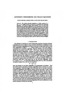
cubic terms resulting from the product of just a single variable. Thus, it seems natural to ask what sort of organization could underly such elusive mixing of variables. Olsen considered the dynamics observed when varying k1 in the interval 0.3 < k1 < 0.41. He computed the phase diagram reproduced in Fig. 1(a), where periodic regimes are denoted by P‘, ‘ being the number of peaks (local maxima) per period of the variable A. Except for the transition region between P2 and P3, other transitions were found to be “sharp,” i.e., without indication of chaos happening between them. Subsequently, Steinmetz et al.27 studied the oscillations supported by the model, reporting a phase diagram spanning the k3  k1 section of the control space, reproduced here in Fig. 1(b). They do not define what they mean by “simple” and “complex” oscillations. Figure 1(c) illustrates a phase diagram obtained by us, classifying with colors the number of peaks per period and, in black, revealing the presence of a (small) chaotic phase. Comparing Figs. 1(b) and 1(c), one sees that, rather than chaos, the “complex” oscillations in Fig. 1(b) correspond predominantly just to periodic oscillations with a growing number of peaks per period. As indicated by the horizontal and vertical sequences of dots, note the equivalence of the unfolding of oscillations obtained when (i) holding k1 fixed and tuning k3 or (ii) holding k3 fixed and tuning k1. Changing both parameters can also produce similar unfoldings along many paths. Figure 1(c) is an example of the high-resolution stability diagrams reported in this paper and Sec. II explains how they are obtained. Section III describes the nested arithmetic progressions and the global organization of stability phases present in several control parameter planes of Olsen’s PO model. Section IV summarizes the four types of arithmetic progressions and their distinctive signatures. Our conclusions and some open problems are present in Sec. V. Generally

FIG. 1. Phase diagrams illustrating the knowledge about stable oscillatory phases according to Olsen’s enzyme reaction model. Numbers denote the number of peaks (local maxima) per period of A. (a) Original phase diagram, after Olsen,23 and (b) phase diagram after Steinmetz et al.,27 discriminating Hopf bifurcations (HBs) and period doubling (PD). Note that their PD boundary is not always accurate. (c) Same as (b) but showing all stable phases. Colors display the number of spikes of A per period. White denotes constant, i.e., non-oscillating (NO) solutions. Black represents non-periodic oscillations (chaos). The white box is magnified in Fig. 2. The vertical line dividing the box marks the k1 interval in panel (a). Coordinates of the dots plotted vertically are given in Table I below.

This article is copyrighted as indicated in the article. Reuse of AIP content is subject to the terms at: http://scitation.aip.org/termsconditions. Downloaded to IP: 143.54.2.243 On: Fri, 22 May 2015 17:01:15

064603-3

M. R. Gallas and J. A. C. Gallas

speaking, note that it is a matter of no little difficulty to distinguish the systematics (if any) of how self-sustained complex oscillatory behaviors organize themselves in the control space of nonlinear oscillators. The understanding of such systematics is our leitmotiv. II. COMPUTATIONAL DETAILS

Stability diagrams like the one in Fig. 1(c) are examples of isospike diagrams,28–33 namely, diagrams recording the number of peaks per period of a given component of the oscillations. Such diagrams are the main tool used here to characterize the unfolding of oscillations in control parameter space. To produce them, a selected parameter window of interest is covered with a mesh of N  N equidistant points. For each point of the mesh, the temporal evolution is obtained by integrating numerically Eqs. (1)–(4) using the standard fourth-order Runge-Kutta algorithm with fixed time-step h ¼ 0.002. In all phase diagrams, integrations were always started from an arbitrarily chosen initial condition, A ¼ B ¼ X ¼ Y ¼ 0.5. The first 16  106 integration steps were disregarded as transient-time needed to approach the attractor. The subsequent 16  106 steps were used to compute the Lyapunov spectrum (not shown here). To find the number of peaks per period, subsequent to the computation of Lyapunov exponents, we continued integrations for an additional 40  105 time-steps recording up to 800 extrema (maxima and minima) of the variable of interest together with the instant when they occur, and recording repetitions of the maxima. When plotting time evolutions, integrations were started from the arbitrary point (A, B, X, Y) ¼ (1, 1, 0.01, 0.01), maintaining all other conditions above. Following earlier works,9,23,27 we select the following default values when parameters are not varying: A0 ¼ 8, B0 ¼ 1, X0 ¼ 1, k1 ¼ 0.38, k2 ¼ 250, k3 ¼ 0.025, k4 ¼ 20, k5 ¼ 5.35, k6 ¼ 105, k7 ¼ 0.1, and k8 ¼ 0.825. As indicated by the colorbar in Fig. 1(c) and similar figures below, a palette of 17 colors is used to represent the number of peaks (local maxima) contained in one period of the oscillations. Patterns with more than 17 peaks are plotted by periodically recycling the 17 basic colors. Multiples 17  ‘ of 17 are plotted with the color index corresponding to (18  ‘) mod 17, namely, 34  16 for ‘ ¼ 2, 51  15 for ‘ ¼ 3, 68  14 for ‘ ¼ 4, etc. Black is used to represent “chaos” (i.e., lack of numerically detectable periodicity), light-pink corresponds to divergent solutions, and white and orange mark non-oscillatory solutions, if any, having, respectively, non-zero or zero amplitudes of the variable under consideration. The computation of stability diagrams is numerically a quite demanding task that we performed using in-house developed FORTRAN software to generate Postscript bitmaps, and with the decisive help of up to 1536 processors of a SGI Altix cluster having a theoretical peak performance of 16 Tflops. While it is possible to observe period-doubling (PD) routes, most of the times what happens is just the addition of a new peak to the waveform (without a corresponding doubling of the period). Note that the period is a quantity that evolves continuously when parameters are changed, while the number of peaks is a “quantized”

Chaos 25, 064603 (2015)

quantity, namely, a quantity that changes in discrete steps. The mechanism responsible for peak addition is described elsewhere.34,35 Eventually, after adding peaks, one may reach a situation where the period roughly doubles a numerical value observed previously. But such coincidence occurs for very specific parameter values, not for parameter intervals. The computation of stability diagrams is a standard calculation that we performed as described in detail, e.g., in Ref. 38 where efficient methods to deal both with numerical and experimental data are given. See also Refs. 39–42. Each panel in Fig. 5 was obtained by analyzing a mesh of N ¼ 600 parameter points. All other phase diagrams are bitmaps displaying individually the analysis of 1200  1200 ¼ 1.44  106 parameters, i.e., of sets containing the analysis of more than a million points in parameter space. To decrease the size of papers, beware that publishers routinely tend to severely reduce the resolution of the figures, something unfortunate and beyond our control that frequently destroys information originally contained in the diagrams. III. NESTED ARITHMETIC PROGRESSIONS

We begin with an alert concerning inaccurate language commonly used when describing bifurcations generated by flows, i.e., by continuous-time dynamical systems. Perioddoubling bifurcation was first described for maps (discretetime systems) where a degenerate situation occurs. Subsequent to period-doubling, the period of maps remains constant over extended parameter windows. In sharp contrast, in flows, the period does not remain constant when parameters are varied. But there are quantities (other than the period) which remain constant over extended parameter intervals, e.g., the number of peaks (local maxima) per period and the number of local minima. Figure 2 displays a series of stripes which, together, form a pair of nested arithmetic progressions of stability phases. Phases are labeled by the number of peaks per period of their oscillations. The progressions are formed by an alternation of wide and narrow stripes. So, there is a main progression formed by wide stripes 2 ! 3 ! 4 ! 5 ! …, and a secondary progression of much narrower stripes 5 ! 7 ! 9 ! … embedded between adjacent stripes of the main progression. In the main progression, the number of peaks increases by one unit, while in the secondary it grows by two units. The number of spikes of a secondary stripe corresponds to the sum of the number of spikes of the stripes adjacent to it (and which belong to the main progression). The two rows on the top of Fig. 3 show typical temporal evolutions of A and B, respectively, as indicated by the labels. The leftmost column shows a time series with 2 peaks, the central column has 5 peaks, while the rightmost column has 3 peaks. These signals are for parameters contained in the regions labeled as 2, 5, and 3 in Fig. 2(a). Clearly, these plots illustrate characteristic time evolutions observed for parameters belonging to both nested progressions: The 5-peaked pattern is the “sum” of its adjacent patterns. The bottom row shows A  B projections of the periodic attractors for the five points labeled as 2, 5, 3, 7, and 4 in Fig. 2(a). These projections show unambiguously the

This article is copyrighted as indicated in the article. Reuse of AIP content is subject to the terms at: http://scitation.aip.org/termsconditions. Downloaded to IP: 143.54.2.243 On: Fri, 22 May 2015 17:01:15

064603-4

M. R. Gallas and J. A. C. Gallas

Chaos 25, 064603 (2015)

FIG. 2. Stability diagrams with color stripes indicating oscillatory phases characterized by the number of peaks per period of the variable A. (a) Enlargement of the white box in Fig. 1(c) indicating the nested sequence of arithmetic progressions: The main sequence 2 ! 3 ! 4 ! 5 ! … of larger stripes, and a secondary sequence 5 ! 7 ! 9 ! … of finer stripes embedded between pairs of stripes of the main progression. The vertical line marks the interval studied by Olsen,23 while the interval indicated by the horizontal line segment was studied by Steinmetz et al.27 The white box is enlarged in Fig. 4. (b) A pair of circles indicating that chaos exists on the tips of the “fingers” of the secondary progression. A similar circle is shown in (a).

concatenated nature of the patterns belonging to the secondary progression. How do transitions between stripes occur? As mentioned, Olsen found that except for chaos observed between the region with 2 and 3 peaks in Fig. 1(a), other transitions were “sharp,” i.e., without indication of chaos happening

between them. However, under high-resolution, we find a distinct picture to emerge. As it may be recognized from the structure of the black chaotic phase in Fig. 2, narrow stripes of chaos exist on both sides of the five peaks “finger” where the secondary progression begins. Such stripes of chaos continue to exist when k1 and k3 increase, as it is visible in

FIG. 3. The two top rows show the temporal evolution of A and B for parameter points inside the first three stripes 2, 5, and 3 in Fig. 2(a), whose coordinates are given in Table I below. Patterns in the middle column (for 5 peaks) correspond to a concatenation of the adjacent patterns, with 2 and 3 peaks. Their periods obey T5  T2 þ T3. The bottom row illustrates A  B projections of the oscillations for the first few points in Fig. 2(a). Two progressions can be easily distinguished: Panels for 2, 3, and 4 peaks belong to the main progression, while panels for 5 and 7 peaks belong to the secondary projection. Note the growing amplitudes of the oscillations, specially B. Progressions between oscillations having 2, 5, 3 peaks were already observed experimentally in the enzyme reaction by Hauser et al.17,18

This article is copyrighted as indicated in the article. Reuse of AIP content is subject to the terms at: http://scitation.aip.org/termsconditions. Downloaded to IP: 143.54.2.243 On: Fri, 22 May 2015 17:01:15

064603-5

M. R. Gallas and J. A. C. Gallas

Fig. 1(c). Stripes of chaos become extremely narrow as k1 and k3 further increase and it is not possible to discern numerically if they disappear or simply become too narrow to be detected. What is clear, however, is that relatively broad chaos exists at the tips of the fingers of the secondary progression. The tip of the next two pairs of fingers from the secondary progression is indicated by circles in Fig. 2(b). They correspond to narrow stripes of oscillations with 7 and 9 peaks. Figure 2(b) does not contain the 2-peaks stripe that is clearly visible in Fig. 2(a). The reason for this is that stripes seem to end in specific regions of the control parameter space and that at such endings the regularities observed elsewhere may be broken in the sense that in these regions the progression of stripes can be truncated, particularly for stripes with fewer number of peaks. Several domains seem to end in the form of a hook. Figure 2 corroborates Olsen’s original description. In particular, with the benefit of hindsight, one may now recognize that the sequence 3–7–4 recorded by Olsen in his Fig. 1(a) corresponds to the portion of the nested arithmetic progressions that lies on the lower part of the vertical line in Fig. 2(a). Figure 2(b) shows that the chaotic phase, although relatively small when compared to the large nearby domains of periodicity, reappears in several other locations. It would be interesting to investigate the mechanism that leads to chaos in these rather specific positions in control parameter space. Subsequently to Olsen,23 Steinmetz et al.27 reported an interesting study of the impact of varying k3, the parameter believed to play a role similar to the important cofactor DCP (i.e., 2,4-dichlorophenol) used in in vitro flow experiments and whose variation resulted in changes in oscillation pattern very similar to those observed in Olsen’s model.9 In their Fig. 6, Steinmetz et al.27 show a sequence of oscillations obtained while holding k1 ¼ 0.35 fixed. They described such sequence as corresponding to a typical period-doubling cascade, starting from an oscillation at low k3 values, through a period-two state, period-four state, and so on until chaos is reached. Chaos consists of a window located roughly in the

Chaos 25, 064603 (2015) TABLE I. Representative points inside the two nested arithmetic progressions. Points in the secondary progression are indicated by asterisks. The six points at the bottom refer to the doubling route discussed by Steinmetz et al.27 See the text. Point 1 2 3 4 5 6 7 8 9 10 11 12 13 14 a b b0 c d e

k3

k1

Peaks

Period

0.051 0.051 0.051 0.051 0.051 0.051 0.051 0.051 0.051 0.051 0.051 0.051 0.051 0.051 0.027 0.033 0.0333 0.0336 0.035 0.038

0.51 0.46 0.415 0.39 0.376 0.36 0.3495 0.338 0.3267 0.318 0.3078 0.298 0.2915 0.284 0.35 0.35 0.35 0.35 0.35 0.35

1 2 5* 3 7* 4 9* 5 11* 6 13* 7 15* 8 1 2 4 8 Chaos 3

11.7845 22.8595 53.8105 30.9710 70.2110 38.6395 85.6520 45.8920 100.3795 52.8180 114.2505 59.4200 127.7075 65.9295 12.6425 23.9785 47.9825 96.0380 Chaos 33.3755

interval of 0.033 < k3 < 0.038, followed by a period-three window. The oscillation for k3 ¼ 0.0336 described in their Fig. 6 does not correspond to period-four but to period-8, apparently invalidating the claim of a doubling route in the region. To elucidate the existence or not of a doubling route along the line k1 ¼ 0.35, in Fig. 4 and in Table I one records the points b, c, d, and e considered by Steinmetz et al.27 As mentioned, although point c is not in the 4-peaks region, there is a continuum of 4-peaks oscillations located roughly in the k3-interval [0.03315, 0.03515] with the period varying in [47.9020, 48.0275], respectively. For the point b0 listed in Table I, we obtain the following rates for the period increase: Tb ¼ 1:8966; Ta

FIG. 4. Stability diagram showing the points reported by Steinmetz et al.27 Colors represent the number of peaks per period, black denotes chaos. When point b0 is added (see Table I), their corrected sequence corresponds to a doubling of the number of peaks (not period) of the oscillations.

Tb0 ¼ 2:0011; Tb

Tc ¼ 2:0015: Tb0

The point b0 was chosen so as to optimize the ratios. As it is clear from Fig. 4, the above ratios will change if one moves either b0 or any of the other points involved to different locations in their windows, making it plain that the periods and their rates change continuously with parameters. Figure 4 shows two additional facts concerning the unfolding of bifurcations. First, when k3 increases, the doubling route reported by Steinmetz et al.27 indeed exists but it is restricted to a rather small window of parameters. Under low-resolution, one may be easily mislead into thinking that the 8-peaks phase is followed by a sharp transition to chaos, what is not the case. Second, Olsen described doubling routes to exist on the boundary of the three-peaks phase when either increasing or decreasing the value of k1. Along this boundary, we find multistability to be abundantly

This article is copyrighted as indicated in the article. Reuse of AIP content is subject to the terms at: http://scitation.aip.org/termsconditions. Downloaded to IP: 143.54.2.243 On: Fri, 22 May 2015 17:01:15

064603-6

M. R. Gallas and J. A. C. Gallas

Chaos 25, 064603 (2015)

FIG. 5. Stability diagrams showing that regular tilings and nested progressions are also observable in other control parameter planes. Multistability is also visible in several regions. Note that between the 4-peak and 5-peak “petals,” or fingers, in panels (b) and (e) there is an accumulation of a large number of similar but smaller fingers. The same is true for other pairs of fingers. In the top row, we fixed k1 ¼ 0.38, while the bottom row is for k3 ¼ 0.025.

present, meaning that it is possible to observe either sharp transitions to chaos or the smooth doubling route. Are nested arithmetic progressions of peak-adding phases observable when tuning other parameters than k1 and k3? Figure 5 shows this to be indeed the case. From the equations of motion, one sees that the three sections k3  k1, k3  k2, and k1  k2 considered here exhaust all possible combinations of the nonlinearities in them. In these three planes, similar phenomena are clearly visible although details of the specific arrangements may differ slightly. An evident characteristic of the structural organization of the stability phases is that their unfolding is too complex to be described by other means than purely graphic. Multistability is also visible in several regions. A detailed investigation of the two additional parameter planes in Fig. 5 remains to be done, as well as the investigation of the several planes involving linear terms in the equations of motion. Figure 6 shows an enlargement of the box in Fig. 2(a), illustrating how complex and diverse the stability striations inside the phase of chaos can be. The structure having 16peaks in the main domain is a shrimp.43–45 The rightmost stripe is in fact a kind of self-connected pair of 19-peaks shrimps. Between these two striations, there is a crossingover of two stability domains with 7 and 12 peaks, as indicated. Under the low resolution of Fig. 2, they all appear to be identical striations embedded in chaos, which is not the case. The classification of these and other striations remains an open challenge. Much more complicated periodic phases

FIG. 6. Magnification of the white box in Fig. 2(a) illustrating the diversity and complexity of the stability stripes living inside the phase of chaos: A shrimp43–45 having 16-peaks in the main stability domain, and a complex folding involving a self-connected structure with 19-peaks, a sort of “double” shrimp. Between them, one finds the crossing-over of two stability domains characterized by 7 and 12 peaks, as indicated.

This article is copyrighted as indicated in the article. Reuse of AIP content is subject to the terms at: http://scitation.aip.org/termsconditions. Downloaded to IP: 143.54.2.243 On: Fri, 22 May 2015 17:01:15

064603-7

M. R. Gallas and J. A. C. Gallas

Chaos 25, 064603 (2015)

exist embedded in the chaotic phases in Fig. 2 but will not be discussed here. IV. TYPES OF NESTED PROGRESSIONS

Section III has shown that arithmetic progressions or, equivalently, adding cascades are organized differently than the familiar geometric progressions associated with doubling cascades. Recall that in maps (discrete-time systems) the quantity undergoing doubling is the period, while for differential equations (continuous-time systems) doubling occurs in the number of peaks per period. Implicitly, underlying the notion of “period doubling” are parameter intervals where the period remains constant. In sharp contrast, no equivalent intervals exist for continuous-time systems (flows) because the period evolves continuously with parameters. In continuous-time systems, a quantity that remains constant along parameter intervals is the number of spikes per period, not the period. Accordingly, period-doubling in maps may be associated to spike-doubling in flows, and vice-versa. Period-doubling, a familiar signature of maps, was discussed theoretically and numerically with high-precision in 1958–1963 by Myrberg using an early version of a computer, an “Elektronenmaschine” as he called it.46–50 With more amplitude and new twists, period doubling was discussed subsequently in 1976 by May,51 in 1977 by Grossmann and Thomae,52 and in 1978 by Coullet and Tresser56,57 and Feigenbaum.58 Adding phenomena in maps were studied in 1982 by Kaneko.53 In experiments, adding phenomena were observed as early as 1927 by van der Pol and van der Mark in a neon discharge.54 Although electronic models of plasma discharges involve differential equations,39 a theoretical investigation of the adding phenomenon motivated by their discharge was provided only much later, in 1990, in a nice paper by Levy55 based, however, on a certain implicit map, not on differential equations. Geometric and arithmetic progressions of stability phases evolve quite differently. In maps, geometric progressions involve periodic orbits forming doubling sequences k‘ ¼ k02‘, for ‘ ¼ 0, 1, 2, 3, …, where k0 is the main period of the window. Transitions between consecutive windows k‘ and k‘ þ 1 are continuous, in the sense that the passage is not mediated by a window of chaos. Doubling cascades end invariably in chaos, i.e., they accumulate towards a phase of chaos. In contrast, arithmetic progressions involve k-periodic phases which grow linearly according to k‘ ¼ k0 þ ‘ Dk, where D ¼ 1, 2, 3, …. This linear growth is usually referred to as period-adding. As seen in Figs. 2 and 5, adding transitions may or may not be mediated by windows of chaos. Adding cascades accumulate towards phases characterized either by a constant period (for maps) or by a constant number of peaks (for flows) as shown in the figures here, in Fig. 5 of Ref. 35 for a CO2 laser with feedback and in Figs. 2 and 4 of Ref. 36 for a damped-driven Duffing oscillator. How many distinct types of arithmetic progressions are there and what are the characteristic signatures to discriminate them in laboratory experiments and with computers? Thus far, we identified four types of adding cascades which are found to exist abundantly over wide parameter windows.

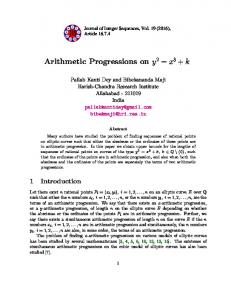
FIG. 7. The fan-like self-similar bridge cascade of nested arithmetic progressions connecting stability domains with k and k þ 1 peaks per period. (a) Peak adding bridging “petals” with 4, 5, 6, … peaks per period. Circles have the same meaning as in Fig. 2(b). (b) Enlargement of the bridge between petals 4 and 5. The bridge is formed by self-similar filamentary phases of an ever growing number of peaks per period, forming a sort of akomeogi. Phases with higher number of peaks accumulate on both sides of every pair of smooth boundaries.

They may be easily distinguished by considering the specific nature of what separates consecutive phases with k and k þ 1 peaks per period. First, the most familiar adding transitions are the ones mediated by windows of chaos, as frequently observed in mixed-mode oscillations.21,22 Second, there are mixed-mode oscillations where windows of chaos are totally absent19,35 (see the previous paragraph). Third, there are the transitions involving concatenated periodic oscillations and nested progressions as described in Figs. 2 and 3. Fourth, there is a beautiful and highly nested type of transition mediated by complex but regular alternations of smaller and smaller phases with an ever growing number of peaks per period that accumulate methodically, as illustrated in Fig. 7(b) and, less clearly, in several panels of Fig. 5. In this transition, individual phases are separated by windows of chaos and form sequences of nested arithmetic progressions ‘ ¼ 1, 2, 3,

This article is copyrighted as indicated in the article. Reuse of AIP content is subject to the terms at: http://scitation.aip.org/termsconditions. Downloaded to IP: 143.54.2.243 On: Fri, 22 May 2015 17:01:15

064603-8

M. R. Gallas and J. A. C. Gallas

…, each one characterized by a constant difference D‘ between consecutive phases. As seen in Fig. 7(b), progressions with peaks increasing by D‘ accumulate towards a larger phase having D‘ peaks per period. These arithmetic progressions are believed to be not restricted to Olsen’s flow but to be also observable in other dynamical systems. Figure 7(b), an enlargement of the small cyan box in Fig. 5(d), shows that between the large “petals,” characterized by oscillations with 4 and 5 peaks per period, there is a complex fan-like self-similar accumulation of a growing number of smaller and smaller fingers. Stability phases between the 9 and 5 petals are arranged in hierarchies of additional progressions which increase by 5 peaks, while between petals 9 and 4 the progressions increase by 4 peaks. The first few phases are indicated by their number of peaks. The next generations display a self-similar arrangement which apparently repeats ad infinitum. The pair of smooth external boundaries of each phase are accumulation lines for hierarchies of phases with higher number of spikes which converge to them on both sides. The fan-like hierarchy of phases seen in Fig. 7(b) exists profusely in other parameter regions. As may be recognized from the stability diagrams above, all four types of arithmetic progressions may coexist in the same dynamical system. Progressions appear in a specific parameter region and seem to evolve continuously from one type into another when parameters are tuned. It would be nice to investigate whether or not fan-like bridges share a common origin with the structural organization observed in maps when phases of complex-valued oscillations are stabilized by real-valued changes in parameters.37 Fan-like bridges seem to play a pervasive role in nonlinear dynamics since we observed them also in a few other systems. These bridges and their filamentary phases are now under investigation. V. CONCLUSION AND OUTLOOK

This paper provided a provisional description of the unfolding of periodic oscillations as seen from sections of the control parameter space of Olsen’s enzyme reaction model. A more encompassing classification of the intricate combinations of chaotic and non-chaotic phases visible in our stability diagrams demands much more investment of computer time and experimentation. Particularly, enticing is to try to understand the generic unfolding of the fan-like scenario of Fig. 7. An open challenge is to classify the unfolding of wave pattern complexification by peak deformation and adding when several parameters are tuned simultaneously. The impact of the linear terms in the equations of motion remains totally unexplored. Olsen’s model involves nine parameter values and it is not immediately obvious that the specific parameter sections considered here are optimal to expose generic trends. Much work remains to be done in order to discover the structural properties of the control parameter space. The aforementioned distinctive product of three variables needs to be found and probed in other models to assess its influence. Hauck and Schneider16 reported experimental observations of the peroxidase-oxidase reaction, in particular, they

Chaos 25, 064603 (2015)

recorded experimental doubling routes to chaos in a Farey sequence by varying the O2 flow. They found that the simple Olsen model shows a similar scenario as the experiments. They reported observing a Farey sequence when changing k7, a rate constant controlling a linear term in the dynamical equations. Although observing just quite limited sequences of oscillations, they interpreted them as belonging to a Farey tree, apparently unaware that the arithmetic sum rule p1/q1 丣 p2/q2 ¼ (p1 þ p2)/(q1 þ q2), which they used as evidence to claim observing the asymmetric Farey tree, is a sum rule that can be used equally well to identify a distinct and much more general organization: the symmetric Stern-Brocot tree.28–30,59 In other words, although frequently used in older literature, fits of the aforementioned arithmetic sum rule to noisy and small sets of data are by no means enough for a conclusive and unambiguous identification of the nature of the underlying organizational tree. Thus, it would be nice to reconsider the experiments and check if they could eventually support the Stern-Brocot scenario. More specifically, to check under higher resolution and for wider range of parameters and resolution whether or not the k7 space is home of Farey or Stern-Brocot trees. In the last four decades, considerable effort has been devoted to studying chaos. But understanding progressions of periodic solutions is as important an issue as chaos. ACKNOWLEDGMENTS

This article is dedicated to Professor Irving R. Epstein on the occasion of his 70th birthday. The authors acknowledge support from CNPq, Brazil. All bitmaps were computed in the CESUP-UFRGS clusters, located in Porto Alegre, Brazil. 1

R. Kremann, Die periodischen Erscheinungen in der Chemie (F. Enke Verlag, Stuttgart, 1913). We have not been able to obtain this reference. 2 E. S. Hedges and J. E. Myers, The Problem of Physico-Chemical Periodicity (Arnold & Co, London, 1926). 3 V. K. Vanag, D. G. Mıguez, and I. R. Epstein, “Designing an enzymatic oscillator: Bistability and feedback controlled oscillations with glucose oxidase in a continuous flow stirred tank reactor,” J. Chem. Phys. 125, 194515 (2006). 4 Oscillations and Traveling Waves in Chemical Systems, edited by R. J. Field and M. Burger (Wiley, New York, 1985). 5 Chemical Waves and Patterns, edited by R. Kapral and K. Showalter (Kluwer, Dordrecht, 1995). 6 Peroxidases in Chemistry and Biology, edited by J. Everse, M. B. Grisham, and K. D. Everse (CRC Press, Cleveland, 1991). 7 S. Strogatz, Nonlinear Dynamics and Chaos with Applications to Physics, Biology, Chemistry, and Engineering, 2nd ed. (Westview Press, Boulder, 2015). 8 J. Argyris, G. Faust, M. Haase, and R. Friedrich, An Exploration of Dynamical Systems and Chaos, 2nd ed. (Springer, New York, 2015). 9 R. Larter, “Understanding complexity in biophysical chemistry,” J. Phys. Chem. B 107, 415–429 (2003). 10 A. F. Taylor, “Mechanism and phenomenology of an oscillating chemical reaction,” Prog. React. Kinet. Mech. 27, 247–325 (2002). 11 M. J. B. Hauser and L. F. Olsen, “Routes to chaos in the peroxidaseoxidase reaction,” Lect. Notes Phys. 532, 252–272 (1999). 12 A. Scheeline, D. L. Olson, E. P. Williksen, G. A. Horras, M. L. Klein, and R. Larter, “The peroxidase-oxidase oscillator and its constituent chemistries,” Chem. Rev. 97, 739–756 (1997). 13 I. R. Epstein and K. Showalter, “Nonlinear chemical dynamics: Oscillations, patterns, and chaos,” J. Phys. Chem. 100, 13132–13147 (1996). 14 R. Larter and C. G. Steinmetz, “Chaos via mixed-mode oscillations,” Philos. Trans. R. Soc., A 337, 291–298 (1991).

This article is copyrighted as indicated in the article. Reuse of AIP content is subject to the terms at: http://scitation.aip.org/termsconditions. Downloaded to IP: 143.54.2.243 On: Fri, 22 May 2015 17:01:15

064603-9 15

M. R. Gallas and J. A. C. Gallas

B. D. Aguda and R. Larter, “Periodic-chaotic sequences in a detailed mechanism of the peroxidase-oxidase reaction,” J. Am. Chem. Soc. 113, 7913–7916 (1991). 16 T. Hauck and F. W. Schneider, “Chaos in a Farey sequence through period doubling in the peroxidase-oxidase reaction,” J. Phys. Chem. 98, 2072–2077 (1994). 17 M. J. B. Hauser and L. F. Olsen, “Mixed-mode oscillations and homoclinic chaos in an enzyme reaction,” J. Chem. Soc., Faraday Trans. 92, 2857–2863 (1996). 18 M. J. B. Hauser, L. F. Olsen, T. V. Bronnikova, and W. M. Schaffer, “Routes to chaos in the peroxidase-oxidase reaction: Period-doubling and period-adding,” J. Phys. Chem. B 101, 5075–5083 (1997). 19 M. J. B. Hauser and J. A. C. Gallas, “Nonchaos-mediated mixed-mode oscillations in an enzyme reaction systems,” J. Phys. Chem. Lett. 5, 4187–4193 (2014). 20 T. V. Bronnikova, V. R. Fedkina, W. M. Schaffer, and L. F. Olsen, “Period-doubling bifurcations and chaos in a detailed model of the peroxidase-oxidase reaction,” J. Phys. Chem. 99, 9309–9312 (1995). 21 M. Brøns, T. J. Kaper, and H. G. Rotstein, “Preface to ‘Mixed mode oscillations: Experiment, computation, and analysis’,” Chaos 18, 015101 (2008). 22 E. J. Doedel and C. L. Pando, “Multiparameter bifurcations and mixedmode oscillations in Q-switched CO2 lasers,” Phys. Rev. E 89, 052904 (2014). 23 L. F. Olsen, “An enzyme reaction with a strange attractor,” Phys. Lett. A 94, 454–457 (1983). 24 J. A. C. Gallas, “The structure of periodic and chaotic hub cascades in phase diagrams of simple autonomous systems,” Int. J. Bifurcation Chaos 20, 197–211 (2010). 25 R. Vitolo, P. Glendinning, and J. A. C. Gallas, “Global structure of periodicity hubs in Lyapunov phase diagrams of dissipative flows,” Phys. Rev. E 84, 016216 (2011). 26 M. A. Nascimento, H. Varela, and J. A. C. Gallas, “Periodicity hubs and spirals in an electrochemical oscillator,” J. Solid State Electrochem. 19 (2015). 27 C. G. Steinmetz, T. Geest, and R. Larter, “Universality in the peroxidaseoxidase reaction: Period doublings, chaos, period three, and unstable limit cycles,” J. Phys. Chem. 97, 5649–5653 (1993). 28 J. G. Freire and J. A. C. Gallas, “Stern-Brocot trees in the periodicity of mixed-mode oscillations,” Phys. Chem. Chem. Phys. 13, 12191–12198 (2011). 29 J. G. Freire and J. A. C. Gallas, “Stern-Brocot trees in cascades of mixedmode oscillations and canards in the extended Bonhoeffer-van der Pol and the FitzHugh-Nagumo models of excitable systems,” Phys. Lett. A 375, 1097–1103 (2011). 30 J. G. Freire, T. P€oschel, and J. A. C. Gallas, “Stern-Brocot trees in spiking and bursting of sigmoidal maps,” Europhys. Lett. 100, 48002 (2012). 31 S. L. T. Souza, A. A. Lima, I. R. Caldas, R. O. Medrano-T., and Z. O. Guimar~aes-Filho, “Self-similarities of periodic structures for a discrete model of a two-gene system,” Phys. Lett. A 376, 1290–1294 (2012). 32 M. R. Gallas, M. R. Gallas, and J. A. C. Gallas, “Distribution of chaos and periodic spikes in a three-cell population model of cancer,” Eur. Phys. J.: Spec. Top. 223, 2131–2144 (2014). 33 A. Hoff, D. T. da Silva, C. Manchein, and H. A. Albuquerque, “Bifurcation structures and transient chaos in a four-dimensional Chua model,” Phys. Lett. A 378, 171–177 (2014). 34 L. Junges and J. A. C. Gallas, “Intricate routes to chaos in the MackeyGlass delayed feedback system,” Phys. Lett. A 376, 2109–2116 (2012).

Chaos 25, 064603 (2015) 35

L. Junges and J. A. C. Gallas, “Frequency and peak discontinuities observed in self-pulsations of a CO2 laser with feedback,” Opt. Commun. 285, 4500 (2012). 36 C. Bonatto, J. A. C. Gallas, and Y. Ueda, “Chaotic phase similarities and recurrences in a damped-driven Duffing oscillator,” Phys. Rev. E 77, 026217 (2008). 37 A. Endler and J. A. C. Gallas, “Mandelbrot-like sets in dynamical systems with no critical points,” C. R. Acad. Sci. Math. (Paris) 342, 681–684 (2006). 38 A. Sack, J. G. Freire, E. Lindberg, T. P€ oschel, and J. A. C. Gallas, “Discontinuous spirals of stable periodic oscillations,” Sci. Rep. 3, 3350 (2013). 39 E. Pugliese, R. Meucci, S. Euzzor, J. G. Freire, and J. A. C. Gallas, “Complex dynamics of a dc glow discharge tube: Experimental modeling and stability diagrams,” Sci. Rep. 5, 08447 (2015). 40 J. G. Freire, R. J. Field, and J. A. C. Gallas, “Relative abundance and structure of chaotic behavior: The nonpolynomial Belousov-Zhabotinsky reaction kinetics,” J. Chem. Phys. 131, 044105 (2009). 41 M. A. Nascimento, J. A. C. Gallas, and H. Varela, “Self-organized distribution of periodicity and chaos in an electrochemical oscillator,” Phys. Chem. Chem. Phys. 13, 441–446 (2011). 42 J. G. Freire, R. Meucci, F. T. Arecchi, and J. A. C. Gallas, “Self-organization of pulsing and bursting in a CO2 laser with opto-electronic feedback,” Chaos 25, 097607 (2015). 43 J. A. C. Gallas, “Structure of the parameter space of the Henon map,” Phys. Rev. Lett. 70, 2714–2717 (1993). 44 E. N. Lorenz, “Compound windows of the Henon-map,” Physica D 237, 1689–1704 (2008). 45 W. Fac¸anha, B. Oldeman, and L. Glass, “Bifurcation structures in twodimensional maps: The endoskeletons of shrimps,” Phys. Lett. A 377, 1264–1268 (2013). 46 P. J. Myrberg, “Iteration der reellen Polynome zweiten Grades I,” Ann. Acad. Sci. Fenn. 256, 1–10 (1958); all Myrberg’s papers cited here are available freely online from http://inaesp.org/Legacy. 47 P. J. Myrberg, “Iteration der reellen Polynome zweiten Grades II,” Ann. Acad. Sci. Fenn. 268, 1–13 (1959). 48 P. J. Myrberg, “Iteration der reellen Polynome zweiten Grades III,” Ann. Acad. Sci. Fenn. 363, 1–18 (1963). 49 P. J. Myrberg, “Sur l’iteration des polynomes reels quadratiques,” J. Math. Pures Appl. 41, 339–351 (1962). 50 M. W. Beims and J. A. C. Gallas, “Accumulation points in nonlinear parameter lattices,” Physica A 238, 225–244 (1997). 51 R. M. May, “Simple mathematical models with very complicated dynamics,” Nature 261, 459–467 (1976). 52 S. Grossmann and S. Thomae, “Invariant distributions and stationary correlation functions of one-dimensional discrete processes,” Z. Naturforsch., A 32, 1353–1363 (1977). 53 K. Kaneko, “On the period-adding phenomena at the frequency locking in a one-dimensional mapping,” Prog. Theor. Phys. 68, 669–672 (1982). 54 B. van der Pol and J. van der Mark, “Frequency demultiplication,” Nature 120, 363–364 (1927). 55 M. Levi, “A period-adding phenomenon,” SIAM J. Appl. Math. 50, 943–955 (1990). 56 P. Coullet and C. Tresser, “Iterations d’endomorphismes et groupe de renormalisation,” J. Phys., Colloq. 39(C5), 25–28 (1978). 57 C. Tresser and P. Coullet, “Iterations d’endomorphismes et groupe de renormalisation,” C. R. Acad. Sci. Paris, Ser. A 287, 577–580 (1978). 58 M. J. Feigenbaum, “Quantitative universality for a class of nonlinear transformations,” J. Stat. Phys. 19, 25–52 (1978). 59 R. Graham, D. Knuth, and O. Patashnik, Concrete Mathematics, 2nd ed. (Addison-Wesley, NY, 1994).

This article is copyrighted as indicated in the article. Reuse of AIP content is subject to the terms at: http://scitation.aip.org/termsconditions. Downloaded to IP: 143.54.2.243 On: Fri, 22 May 2015 17:01:15