Nov 22, 2015 - Middle: success probabilities PC (α) adjusted for classical repetition. .... drop in the peak performance at C = 5 relative to the peak observed for ...
Nested Quantum Annealing Correction Walter Vinci,1, 2, 3 Tameem Albash,2, 3, 4 and Daniel A. Lidar1, 2, 3, 5 1
arXiv:1511.07084v1 [quant-ph] 22 Nov 2015
2
Department of Electrical Engineering, University of Southern California, Los Angeles, California 90089, USA Department of Physics and Astronomy, University of Southern California, Los Angeles, California 90089, USA 3 Center for Quantum Information Science & Technology, University of Southern California, Los Angeles, California 90089, USA 4 Information Sciences Institute, University of Southern California, Marina del Rey, California 90292, USA 5 Department of Chemistry, University of Southern California, Los Angeles, California 90089, USA We present a general error-correcting scheme for quantum annealing that allows for the encoding of a logical qubit into an arbitrarily large number of physical qubits. Given any Ising model optimization problem, the encoding replaces each logical qubit by a complete graph of degree C, representing the distance of the errorcorrecting code. A subsequent minor-embedding step then implements the encoding on the underlying hardware graph of the quantum annealer. We demonstrate experimentally that the performance of a D-Wave Two quantum annealing device improves as C grows. We show that the performance improvement can be interpreted as arising from an effective increase in the energy scale of the problem Hamiltonian, or equivalently, an effective reduction in the temperature at which the device operates. The number C thus allows us to control the amount of protection against thermal and control errors, and in particular, to trade qubits for a lower effective temperature that scales as C −η , with η ≤ 2. This effective temperature reduction is an important step towards scalable quantum annealing.
Quantum annealing (QA) attempts to exploit quantum fluctuations to solve computational problems faster than it is possible with classical computers [1–7]. As an approach designed to solve optimization problems, QA is a special case of adiabatic quantum computation (AQC) [8], a universal model of quantum computing [9–12]. In AQC, a system is designed to follow the instantaneous ground state of a time-dependent Hamiltonian whose final ground state encodes the solution to the problem of interest. This results in a certain amount of stability, since the system can thermally relax to the ground state after an error, as well as resilience to errors, since the presence of a finite energy gap suppresses thermal and dynamical excitations [13–18]. Despite this inherent robustness to certain forms of noise, AQC requires error-correction to ensure scalability, just like any other form of quantum information processing [19]. Various error correction proposals for AQC and QA have been made [20–33], but an accuracy-threshold theorem for AQC is not yet known, unlike in the circuit model (e.g., [34]). A direct AQC simulation of a fault-tolerant quantum circuit leads to many-body (high-weight) operators that are difficult to implement [23, 24] or myriad other problems [12]. Nevertheless, a scalable method to reduce the effective temperature would go a long way towards approaching the ideal of closedsystem AQC, where only non-adiabatic transitions constitute the source of errors. Motivated by the availability of commercial QA devices featuring hundreds of qubits [35–38], we focus on error correction for QA. There is a consensus that these devices are significantly and adversely affected by decoherence, noise, and control errors [39–46], which makes them particularly interesting for the study of tailored, practical error correction techniques. Such techniques, known as quantum annealing correction (QAC) schemes, have already been experimentally shown to significantly improve the performance of quantum annealers [26, 30–32], and theoretically analyzed using a mean-field approach [33]. However, these QAC schemes are not easily
generalizable to arbitrary optimization problems since they induce an encoded graph that is typically of a lower degree than the qubit-connectivity graph of the physical device. Moreover, they typically impose a fixed code distance, which limits their efficacy. To overcome these limitations, here we present a family of error-correcting codes for QA, based on a “nesting” scheme, that has the following properties: (1) it can handle arbitrary Ising-model optimization problem, (2) it can be implemented on present-day QA hardware, and (3) it is capable of an effective temperature reduction controlled by the code distance. Our “nested quantum annealing correction” (NQAC) scheme thus provides a very general and practical tool for error correction in quantum optimization. We test NQAC by studying antiferromagnetic complete graphs numerically, as well as on a D-Wave Two (DW2) processor featuring 504 flux qubits connected by 1427 tunable composite qubits acting as Ising-interaction couplings, arranged in a non-planar Chimera-graph lattice [47] (complete graphs were also studied for a spin glass model in Ref. [48]). We demonstrate that our encoding schemes yields a steady improvement for the probability of reaching the ground state as a function of the nesting level, even after minor-embedding the complete graph onto the physical graph of the quantum annealer. We also demonstrate that NQAC outperforms classical repetition code schemes that use the same number of physical qubits.
I.
QUANTUM ANNEALING AND ENCODING THE HAMILTONIAN
In QA the system undergoes an evolution governed by the following time-dependent, transverse-field Ising Hamiltonian: H(t) = A(t)HX + B(t)HP ,
t ∈ [0, tf ] ,
(1)
2 with respectively monotonically decreasing and increasing “annealing schedules” A(t) and B(t). The “driver HamiltoP nian” HX = − i σix is a transverse field whose amplitude controls the tunneling rate. The solution to an optimization problem of interest is encoded in the ground state of the Ising problem Hamiltonian HP , with X X HP = hi σiz + Jij σiz σjz , (2) i∈V
1
1
1
1
1
1
1
1
(i,j)∈E
where the sums run over the weighted vertices V and edges E of a graph G = (V, E), and σix,z denote the Pauli operators acting on qubit i. The D-Wave devices use an array of superconducting flux qubits to physically realize the system described in Eqs. (1) and (2) on a fixed “Chimera” graph (see Fig. 1) with programmable local fields {hi }, couplings {Jij }, and annealing time tf [36–38]. For closed systems, the adiabatic theorem [49, 50] guarantees that if the system is initialized in the ground state of H(0) = A(0)HX , a sufficiently slow evolution relative to the inverse minimum gap of H(t) will take the system with high probability to the ground state of the final Hamiltonian H(tf ) = B(tf )HP . Dynamical errors then arise due to diabatic transitions, but they can be made arbitrarily small via boundary cancellation methods that control the smoothness of A(t) and B(t), as long as the adiabatic condition is satisfied [51–53]. For open systems, specifically a system that is weakly coupled to a thermal environment, the final state is a mixed state ρ(tf ) that is close to the Gibbs state associated with H(tf ) if equilibration is reached throughout the annealing process [18, 54, 55]. In the adiabatic limit the open system QA process is thus better viewed as a Gibbs distribution sampler. The main goal of QAC is to suppress the associated thermal errors and restore the ability of QA to act as a ground state solver. In addition QAC should suppress errors due to noise-driven deviations in the specification of HP [25]. Error correction is achieved in QAC by mapping the logical Hamiltonian H(t) to an appropriately chosen encoded Hamil¯ tonian H(t): ¯ ¯P , H(t) = A(t)HX + B(t)H
t ∈ [0, tf ] ,
(3)
¯ larger than the number defined over a set of physical qubits N ¯ P also includes penalty of logical qubits N = |V|. Note that H terms, as explained below. The logical ground state of HP is extracted from the encoded system’s state ρ¯(tf ) through an appropriate decoding procedure. A successful error correction scheme should recover the logical ground state with a higher probability than a direct implementation of HP , or than a classical repetition code using the same number of physical qubits ¯ . Due to practical limitations of current QA devices that preN vent the encoding of HX , only HP is encoded in QAC. In order to allow for the most general N -variable Ising optimization problem, we now define an encoding procedure for problem Hamiltonians HP supported on a complete graph KN . The first step of our construction involves a “nested” ˜ P that is defined by embedding the logical KN Hamiltonian H into a larger KC×N . The integer C is the “nesting level” and controls the amount of hardware resources (qubits, couplers,
(a) Logical graph: 1st level. 2
(b) 1st level ME. 2
2
3
1
2
2
4
4
4
4
1
1
1
4
2
2
3
2
3
4
4
1
2
4
1 3
2
(c) Nested graph: 4th level.
1
1
4 4
1
3 1
1
3
1
1
3
4
3
3 1
3
1
1 3
2 1
1
4 4
3 4
3
3 1
1
2
4
2 3
2 3
2
4
4
4
4
4
2 3
3
1
2
2
3
3 4
1 2
2
2 3
4 2
4
4 2
2
1
1 3
3
3
(d) 4th level ME.
FIG. 1. Illustration of the nesting scheme. In the left column, a Clevel nested graph is constructed by embedding a KN into a KC×N , with N = 4 and C = 1 (top) and C = 4 (bottom). Red, thick couplers are energy penalties defined on the nested graph between the (i, c) nested copies of each logical qubit i. The right column shows the nested graphs after ME on the DW2 Chimera graph. Brown, thick couplers correspond to the ferromagnetic chains introduced in the process.
˜ P is and local fields) used to represent the logical problem. H constructed as follows. Each logical qubit i (i = 1, . . . , N ) is represented by a C-tuple of encoded qubits (i, c), with c = 1, . . . , C. The “nested” couplers J˜(i,c),(j,c0 ) and local ˜ (i,c) are then defined as follows: fields h J˜(i,c),(j,c0 ) = Jij , ∀c, c0 , i 6= j , ˜ (i,c) = Chi , ∀c, i , h J˜(i,c),(i,c0 ) = −γ , ∀c 6= c0 .
(4a) (4b) (4c)
This construction is illustrated in the left column of Fig. 1. Each logical coupling Jij has C 2 copies J˜(i,c),(j,c0 ) , thus boosting the energy scale at the encoded level by a factor of ˜ (i,c) ; the factor C in C 2 . Each local field hi has C copies h Eq. (4b) ensures that the energy boost is equalized with the couplers. For each logical qubit i, there are C(C − 1)/2 ferromagnetic couplings J˜(i,c),(i,c0 ) of strength γ > 0 (to be optimized), representing energy penalties that promote agreement among the C encoded qubits, i.e., that bind the C-tuple as a single logical qubit i. The second step of our construction is to implement the ˜ P on given QA hardware, with a fully connected problem H
3 1
7
0.8
6 5
0.7
4
0.6 3
0.5
2
0.4
1 C
-4
-3
-2
-1
0
log10 (,)
8
1.8
0.9
7
1.5
0.8
6 5
0.7
4
0.6 3
0.5
log10 (7C )
8
Success Probability
Success Probability
1 0.9
SQA: No ME, < = 0 SQA: Choi ME, < = 0:05 SQA: DW2 ME, < = 0:05 DW2 data
1
0.5
2
0.4
1 C
-3
-2
-1
log10 (,=7C )
0
1
0 0
0.5
1
log10 (C 2 )
1.5
1.8
FIG. 2. Experimental and numerical results for the antiferromagnetic K4 , after encoding, followed by ME and decoding. Left: DW2 success probabilities PC (α) for eight nesting levels C. Increasing C generally increases PC (α) at fixed α. Middle: Rescaled PC (αµC ) data, exhibiting data-collapse. Right: scaling of the energy boost µC vs the maximal energy boost µmax C , for both the DW2 and SQA. Purple circles: DW2 results. Blue stars: SQA for the case of no ME (i.e., for the problem defined directly over KC×N and no coupler noise). Red up-triangles: SQA for the Choi ME [56] (for a full Chimera graph), with σ = 0.05 Gaussian noise on the couplings. Yellow right-triangles: SQA for the DW2 heuristic ME [57, 58] (applied to a Chimera graph with 8 missing qubits) with σ = 0.05 Gaussian noise on the couplings. The flattening of µC suggests that the energy boost becomes less effective at large C. However, this can be remedied by increasing the number of SQA sweeps (see Appendix C), fixed here at 104 . Thus the lines represent best fits to only the first four data points, with slopes 0.98, 0.91, 0.62 and 0.69 respectively. In all panels Nphys ∈ [8, 288].
lower-degree qubit connectivity graph. This requires a minor embedding (ME) [56–60]. The procedure involves replac˜ P by a ferromagnetically-coupled chain ing each qubit in H ˜ P are represented by of qubits, such that all couplings in H inter-chain couplings. The intra-chain coupling represents another energy penalty that forces the chain qubits to behave as a single logical qubit. The physical Hamiltonian obtained af¯ P . We can ter this ME step is the final encoded Hamiltonian H minor-embed a KC×N nested graph representing each qubit (i, c) as a physical chain of length L = dCN/4e + 1 on the Chimera graph [56]. This is illustrated in the right column of Fig. 1. The number of physical qubits necessary for a ME of a KC×N is NCphys = CN L ∼ C 2 N 2 /4. At the end of a QA run implementing the encoded Hamil¯ P and a measurement of the physical qubits, a tonian H decoding procedure must be employed to recover the logical state. For the sake of simplicity we only consider majority vote decoding over both the length-L chain of each encoded qubit (i, c) and the C encoded qubits comprising each logical qubit i (decoding over the length-L chain first, then over the C encoded qubits, does not affect performance; seeAppendix A). The encoded and logical qubits can thus be viewed as forming repetition codes with, respectively, distance L and C. Other decoding strategies are possible wherein the encoded or logical qubits do not have this simple interpretation; e.g., energy minimization decoding, which tends to outperform majority voting [31]. In the unlikely event of a tie, we assign a random value of +1 or −1 to the logical qubit.
II.
RESULTS
Free energy – Using a mean-field analysis similar to the approach pursued in Ref. [33] we can compute the partition
function associated with the nested Hamiltonian A(t)HX + ˜ P for the case with uniform antiferromagnetic couB(t)H plings. This leads to the following free energy density in the low temperature and thermodynamic limits (see Appendix B): � �q 2 2 [A(t)/C] + [2γB(t)m] − γB(t)m2 (5) βF = C 2 β where m is the mean-field magnetization. There are two key noteworthy aspects of this result. First, the driver term is rescaled as A(t) 7→ C −1 A(t). This shifts the crossing between the A and B annealing schedules to an earlier point in the evolution and is related to the fact that QAC encodes only the problem Hamiltonian term proportional to B(t). Consequently the quantum critical point is moved to earlier in the evolution, which benefits QAC since the effective energy scale at this new point is higher [33]. Second, the inverse temperature is rescaled as β 7→ C 2 β. This corresponds to an effective temperature reduction by C 2 , a manifestly beneficial effect. The same conclusion, of a lower effective temperature, is reached by studying the numerically computed success probability associated with thermal distributions (see Appendix C). We shall demonstrate that this prediction is born out by our experimental results, though it is masked to some extent by complications arising from the ME and noise. NQAC results – The hardness of an Ising optimization problem, using a QA device, is controlled by its size N as well as by an overall energy scale α [42]. The smaller this energy scale, the higher the effective temperature and the more susceptible QA becomes to (dynamical and thermal) excitations out of the ground state and misspecification noise on the problem Hamiltonian. This provides us with an opportunity to test NQAC. Since in our experiments we were limited by the largest complete graph that can be embedded on the DW2 device, a K32 (see Appendix D for details), we tuned the hardness of a problem by studying the performance of NQAC as
0.8 3
0.6 0.4
2
0.2 1 C
-3
-2.5
-2
-1.5
log10 (,)
-1
-0.5
0
1
1
2
5
4
0.8 3
0.6 0.4
2
0.2
0.8 0.6
1.5
log10 (7C)
Success Probability
4
Success Probability
1
Normalized Success Probability
4
4
1
0.5
0.4
3
0 0
0.5
1
1.5
2
log10 (C 2 )
2
0.2
1
1 C
C
-3
-2.5
-2
-1.5
log10 (,)
-1
-0.5
0
-3
-2.5
-2
-1.5
-1
-0.5
0
log10 (,)
FIG. 3. Random antiferromagnetic K8 : experimental and numerical results. Left: success probabilities PC (α) for four nesting levels. Middle: success probabilities PC0 (α) adjusted for classical repetition. Right: numerical results for SQA simulations with 20000 sweeps, σ = 0.05 Gaussian noise on the couplings, and with the Choi embedding, showing five nesting levels. Inset: scaling of the energy boost µC vs the maximal energy boost µmax C , for both the DW2 and SQA. Yellow circles: DW2 results. Blue crosses and red up-triangles: SQA for the Choi ME with 10000 (crosses) and 20000 (up-triangles) sweeps, and with σ = 0.05 Gaussian noise on the couplings. The flattening of µC for C > 4 suggests that the energy boost becomes less effective at large C, but increasing the number of sweeps recovers the effectiveness. The lines represent best fits to only the first four data points, with respective slopes η/2 = 0.65, 0.75, and 0.85.
a function of α via HP 7→ αHP , with 0 < α ≤ 1. Note that we did not rescale γ; instead γ was optimized for optimal post-decoding performance (see Appendix E). It is known that for the DW2, intrinsic coupler control noise can be taken to be Gaussian with standard deviation σ ∼ 0.05 of the maximum value for the couplings [45]. Thus we may expect that, without error correction, Ising problems with α . 0.05 are dominated by control noise. We applied NQAC to completely antiferromagnetic (hi = 0 ∀i) Ising problems over K4 (Jij = 1 ∀i, j), and K8 (random Jij ∈ [0.1, 1] with steps of 0.1) with nesting up to C = 8 and C = 4, respectively. We denote by PC (α) the probability to obtain the logical ground state at energy scale α for the C-level nested implementation (see Appendix A for data collection methods). The experimental QA data in Fig. 2 (left) shows a monotonic increase of PC (α) as a function of the nesting level C over a wide range of energy scales α. As expected, PC (α) drops from PC (1) = 1 (solution always found) to PC (0) = 6/16 (random sampling of 6 ground states, where 4 out of the 6 couplings are satisfied, out of a total of 16 states). Note that P1 (α) (no nesting) drops by ∼ 50% when α ∼ 0.1, which is consistent with the aforementioned σ ∼ 0.05 control noise level, while P8 (α) exhibits a similar drop only when α ∼ 0.01. This suggests that NQAC is particularly effective in mitigating the two dominant effects that limit the performance of quantum annealers: thermal excitations and control errors. To investigate this more closely, the middle panel of Fig. 2 shows that the data from the left panel can be collapsed via PC (α) 7→ PC (α/µC ), where µC is an empirical rescaling factor discussed below (see also Appendix F). This implies that P1 (µC α) ≈ PC (α), and hence that the performance enhancement obtained at nesting level C can be interpreted as an energy boost α 7→ µC α with respect to an implementation without nesting. The existence of this energy boost is a key feature of NQAC, as anticipated above. Recall [Eq. (4)] that a nested
graph KC×N contains C 2 equivalent copies of the same logical coupling Jij . Hence a level-C nesting before ME max = C η , with can provide a maximal energy boost µmax C η max = 2. This simple argument agrees with the reduction of the effective temperature by C 2 based on the calculation of the free energy (5). The right panel of Fig. 2 shows µC as a η function of µmax C , yielding µC ∼ C with η ≈ 1.37 (purple max circles). To understand why η < η , we performed simulated quantum annealing (SQA) simulations (see Appendix G for details). We observe in Fig. 2 (right) that without ME and (blue stars). control errors, the boost scaling matches µmax C When including ME and control errors a performance drop results (red triangles). Both factors thus contribute to the sub-optimal energy boost observed experimentally. However, the optimal energy boost is recovered for a fully thermalized state with a sufficiently large penalty (see Appendix C). To match the experimental DW2 results using SQA we replace the Choi ME designed for full Chimera graphs [56] by the heuristic ME designed for Chimera graphs with missing qubits [57, 58], and achieve a near match (yellow triangles) (see Appendix D for more details on ME). Performance of NQAC vs classical repetition – Recall that NCphys = CN L is the total number of physical qubits used at nesting level C; let Cmax denote the highest nesting level that can be accommodated on the QA device for a given KN , i.e., Cmax N L ≤ Ntot < (Cmax + 1)N L, where Ntot is the total number of physical qubits (504 in our experiments). Then MC = bNCphys /NCphys c is the number of max copies that can be implemented in parallel. For NQAC at level C to be useful, it must be more effective than a classical repetition scheme where MC copies of the problem are implemented in parallel. If a single implementation has success probability PC (α), the probability to succeed at least once with MC statistically independent implementations is PC0 (α) = 1 − [1 − PC (α)]MC . It turns out that the antiferromagnetic K4 problem, for which a random guess succeeds
5 with probability 6/16, is too easy [i.e., PC0 (α) approaches 1 too rapidly], and we therefore consider a harder problem: an antiferromagnetic K8 instance with couplings randomly generated from the set Jij ∈ {0.1, 0.2, . . . , 0.9, 1} (see Appendix E for more details and data on this and additional instances). Problems of this type turn out to have a sufficiently low success probability for our purposes, and can still be nested up to C = 4 on the DW2 processor. Results for PC (α) are shown in Fig. 3 (left), and again increase monotonically with C, as in the K4 case. For each C, PC (α) peaks at a value of α for which the maximum allowed strength of the energy penalties γ = 1 is optimal (γ > 1 would be optimal for larger α, as shown in Appendix E; the growth of the optimal penalty with problem size, and hence chain length, is a typical feature of minor-embedded problems [48]). An energy-boost interpretation of the experimental data of Fig. 3 is possible for α values to the left of the peak; to the right of the peak, the performance is hindered by the saturation of the energy penalties. Figure 3 (middle) compares the success probabilities PC0 (α) adjusted for classical repetition, where we have set Cmax = 4, and shows that P20 (α) > P10 (α), i.e., even after accounting for classical parallelism C = 2 performs better than C = 1. However, we also find that P40 (α) < P30 (α) ≤ P20 (α), so no additional gain results from increasing C in our experiments. This can be attributed to the fact that even the K8 problem still has a relatively large P1 (α). Experimental tests on QA devices with more qubits will thus be important to test the efficacy of higher nesting levels on harder problems.
III.
DISCUSSION
Nested QAC offers several significant improvements over previous approaches to the problem of error correction for QA. It is a flexible method that can be used with any optimization problem, and allows the construction of a family of codes with arbitrary code distance. We have given experimental and numerical evidence that nesting is effective by performing studies with a D-Wave QA device and numerical simulations. We have demonstrated that the protection from errors provided by NQAC can be interpreted as arising from an increase (with nesting level C) in the energy scale at which the logical problem is implemented. This represents a very useful tradeoff: the effective temperature drops as we increase the number of qubits allocated to the encoding, so that these two resources can be traded. Thus NQAC can be used to combat thermal excitations, which are the dominant source of errors in QA, and are the bottleneck for scalable QA implementations. We have also demonstrated that an appropriate nesting level can outperform classical repetition with the same number of qubits, with improvements to be expected when next-generation QA devices with larger numbers of physical qubits become available. We, therefore, believe that our results are of immediate and near-future practical use, and constitute an important step toward scalable QA.
ACKNOWLEDGEMENTS
To test the effect of increasing C, and also to study the effect of varying the annealing time, we present in Fig. 3 (right) the performance of SQA on a random K8 antiferromagnetic instance with the Choi ME. The results are qualitatively similar to those observed on the DW2 processor with the heuristic ME [Fig. 3 (left)]. Interestingly, we observe a drop in the peak performance at C = 5 relative to the peak observed for C = 4. We attribute this to both a saturation of the energy penalties and a suboptimal number of sweeps. The latter is confirmed in Fig. 3 (right, inset), where we observe that the scaling of µC with C is better for the case with more sweeps, i.e., again µC ∼ C η , and η increases with the number of sweeps.
We thank Prof. Hidetoshi Nishimori and Dr. Shunji Matsuura for valuable comments, and Dr. Aidan Roy for providing the minor embeddings used in the experiments with the D-Wave Two. Access to the D-Wave Two was made available by the USC-Lockheed Martin Quantum Computing Center. Part of the computing resources were provided by the USC Center for High Performance Computing and Communications. This work was supported under ARO grant number W911NF12-1-0523, ARO MURI Grant Nos. W911NF-11-1-0268 and W911NF-15-1-0582, and NSF grant number INSPIRE1551064.
[1] Kadowaki, T. & Nishimori, H. Quantum annealing in the transverse Ising model. Phys. Rev. E 58, 5355 (1998). [2] Brooke, J., Bitko, D., F., T., Rosenbaum & Aeppli, G. Quantum Annealing of a Disordered Magnet. Science 284, 779–781 (1999). URL http://www.sciencemag.org/ content/284/5415/779.abstract. [3] Brooke, J., Rosenbaum, T. F. & Aeppli, G. Tunable quantum tunnelling of magnetic domain walls. Nature 413, 610–613 (2001).
[4] Farhi, E. et al. A Quantum Adiabatic Evolution Algorithm Applied to Random Instances of an NP-Complete Problem. Science 292, 472–475 (2001). URL http://www. sciencemag.org/content/292/5516/472. [5] Morita, S. & Nishimori, H. Mathematical foundation of quantum annealing. J. Math. Phys. 49, 125210–47 (2008). [6] Das, A. & Chakrabarti, B. K. Colloquium: Quantum annealing and analog quantum computation. Rev. Mod. Phys. 80, 1061– 1081 (2008).
6 [7] S. Suzuki and A. Das (guest eds.). Discussion and Debate - Quantum Annealing: The Fastest Route to Quantum Computation? Eur. Phys. J. Spec. Top. 224, 1 (2015). URL http://epjst.epj.org/articles/ epjst/abs/2015/01/contents/contents.html. [8] Farhi, E., Goldstone, J., Gutmann, S. & Sipser, M. Quantum Computation by Adiabatic Evolution. arXiv:quant-ph/0001106 (2000). URL http://arxiv.org/abs/quant-ph/ 0001106. [9] Aharonov, D. et al. Adiabatic Quantum Computation is Equivalent to Standard Quantum Computation. SIAM J. Comput. 37, 166–194 (2007). [10] Mizel, A., Lidar, D. A. & Mitchell, M. Simple Proof of Equivalence between Adiabatic Quantum Computation and the Circuit Model. Phys. Rev. Lett. 99, 070502 (2007). URL http://link.aps.org/doi/10.1103/ PhysRevLett.99.070502. [11] Gosset, D., Terhal, B. M. & Vershynina, A. Universal Adiabatic Quantum Computation via the Space-Time Circuit-toHamiltonian Construction. Phys. Rev. Lett. 114, 140501– (2015). URL http://link.aps.org/doi/10.1103/ PhysRevLett.114.140501. [12] Lloyd, S. & Terhal, B. Adiabatic and Hamiltonian computing on a 2D lattice with simple 2-qubit interactions. arXiv:1509.01278 (2015). URL http://arXiv.org/ abs/1509.01278. [13] Childs, A. M., Farhi, E. & Preskill, J. Robustness of adiabatic quantum computation. Phys. Rev. A 65, 012322 (2001). [14] Sarandy, M. S. & Lidar, D. A. Adiabatic Quantum Computation in Open Systems. Phys. Rev. Lett. 95, 250503– (2005). URL http://link.aps.org/doi/10.1103/ PhysRevLett.95.250503. [15] Amin, M. H. S., Love, P. J. & Truncik, C. J. S. Thermally Assisted Adiabatic Quantum Computation. Phys. Rev. Lett. 100, 060503 (2008). [16] Lloyd, S. Robustness of Adiabatic Quantum Computing. arXiv:0805.2757 (2008). URL http://arXiv.org/abs/ 0805.2757. [17] Amin, M. H. S., Averin, D. V. & Nesteroff, J. A. Decoherence in adiabatic quantum computation. Phys. Rev. A 79, 022107 (2009). URL http://link.aps.org/doi/10.1103/ PhysRevA.79.022107. [18] Albash, T. & Lidar, D. A. Decoherence in adiabatic quantum computation. Phys. Rev. A 91, 062320– (2015). URL http://link.aps.org/doi/10.1103/ PhysRevA.91.062320. [19] Lidar, D. & Brun, T. (eds.). Quantum Error Correction (Cambridge University Press, Cambridge, UK, 2013). URL http: //www.cambridge.org/9780521897877. [20] Jordan, S. P., Farhi, E. & Shor, P. W. Error-correcting codes for adiabatic quantum computation. Phys. Rev. A 74, 052322 (2006). URL http://link.aps.org/doi/10.1103/ PhysRevA.74.052322. [21] Lidar, D. A. Towards Fault Tolerant Adiabatic Quantum Computation. Phys. Rev. Lett. 100, 160506 (2008). URL http://link.aps.org/doi/10.1103/ PhysRevLett.100.160506. [22] Quiroz, G. & Lidar, D. A. High-fidelity adiabatic quantum computation via dynamical decoupling. Phys. Rev. A 86, 042333 (2012). [23] Young, K. C., Sarovar, M. & Blume-Kohout, R. Error Suppression and Error Correction in Adiabatic Quantum Computation: Techniques and Challenges. Phys. Rev. X 3, 041013– (2013). URL http://link.aps.org/doi/10.1103/
PhysRevX.3.041013. [24] Sarovar, M. & Young, K. C. Error suppression and error correction in adiabatic quantum computation: non-equilibrium dynamics. New J. of Phys. 15, 125032 (2013). URL http:// stacks.iop.org/1367-2630/15/i=12/a=125032. [25] Young, K. C., Blume-Kohout, R. & Lidar, D. A. Adiabatic quantum optimization with the wrong Hamiltonian. Phys. Rev. A 88, 062314– (2013). URL http://link.aps.org/ doi/10.1103/PhysRevA.88.062314. [26] Pudenz, K. L., Albash, T. & Lidar, D. A. Error-corrected quantum annealing with hundreds of qubits. Nat. Commun. 5, 3243 (2014). URL dx.doi.org/10.1038/ncomms4243. [27] Ganti, A., Onunkwo, U. & Young, K. Family of [[6k,2k,2]] codes for practical, scalable adiabatic quantum computation. Phys. Rev. A 89, 042313– (2014). URL http://link.aps. org/doi/10.1103/PhysRevA.89.042313. [28] Bookatz, A. D., Farhi, E. & Zhou, L. Error suppression in Hamiltonian-based quantum computation using energy penalties. Physical Review A 92, 022317– (2015). URL http://link.aps.org/doi/10.1103/ PhysRevA.92.022317. [29] Mizel, A. Fault-tolerant, Universal Adiabatic Quantum Computation. arXiv:1403.7694 (2014). URL http://arXiv. org/abs/1403.7694. [30] Pudenz, K. L., Albash, T. & Lidar, D. A. Quantum annealing correction for random Ising problems. Phys. Rev. A 91, 042302 (2015). URL http://link.aps.org/doi/10.1103/ PhysRevA.91.042302. [31] Vinci, W., Albash, T., Paz-Silva, G., Hen, I. & Lidar, D. A. Quantum annealing correction with minor embedding. Phys. Rev. A 92, 042310– (2015). URL http://link.aps.org/ doi/10.1103/PhysRevA.92.042310. [32] Mishra, A., Albash, T. & Lidar, D. Performance of two different quantum annealing correction codes. arXiv:1508.02785 (2015). URL http://arXiv.org/abs/1508.02785. [33] Matsuura, S., Nishimori, H., Albash, T. & Lidar, D. A. Mean Field Analysis of Quantum Annealing Correction. arXiv:1510.07709 (2015). URL http://arXiv.org/ abs/1510.07709. [34] Aliferis, P., Gottesman, D. & Preskill, J. Quantum accuracy threshold for concatenated distance-3 codes. Quantum Inf. Comput. 6, 97 (2006). URL http://www.rintonpress. com/xqic6/qic-6-2/097-165.pdf. [35] Johnson, M. W. et al. Quantum annealing with manufactured spins. Nature 473, 194–198 (2011). [36] Johnson, M. W. et al. A scalable control system for a superconducting adiabatic quantum optimization processor. Superconductor Science and Technology 23, 065004 (2010). URL http://stacks.iop.org/0953-2048/ 23/i=6/a=065004. [37] Berkley, A. J. et al. A scalable readout system for a superconducting adiabatic quantum optimization system. Superconductor Science and Technology 23, 105014 (2010). URL http:// stacks.iop.org/0953-2048/23/i=10/a=105014. [38] Harris, R. et al. Experimental investigation of an eight-qubit unit cell in a superconducting optimization processor. Phys. Rev. B 82, 024511 (2010). [39] Boixo, S. et al. Evidence for quantum annealing with more than one hundred qubits. Nat. Phys. 10, 218–224 (2014). [40] Shin, S. W., Smith, G., Smolin, J. A. & Vazirani, U. How “Quantum” is the D-Wave Machine? arXiv:1401.7087 (2014). URL http://arXiv.org/abs/1401.7087. [41] Albash, T., Rønnow, T. F., Troyer, M. & Lidar, D. A. Reexamining classical and quantum models for the D-Wave One pro-
7
[42]
[43]
[44]
[45]
[46]
[47]
[48]
[49] [50]
[51]
[52] [53]
[54]
[55]
[56]
[57]
[58]
cessor. Eur. Phys. J. Spec. Top. 224, 111–129 (2015). URL dx.doi.org/10.1140/epjst/e2015-02346-0. Albash, T., Vinci, W., Mishra, A., Warburton, P. A. & Lidar, D. A. Consistency tests of classical and quantum models for a quantum annealer. Phys. Rev. A 91, 042314– (2015). URL http://link.aps.org/doi/10.1103/ PhysRevA.91.042314. Crowley, P. J. D., Duri´c, T., Vinci, W., Warburton, P. A. & Green, A. G. Quantum and classical dynamics in adiabatic computation. Phys. Rev. A 90, 042317– (2014). URL http://link.aps.org/doi/10.1103/ PhysRevA.90.042317. Martin-Mayor, V. & Hen, I. Unraveling Quantum Annealers using Classical Hardness. arXiv:1502.02494 (2015). URL http://arXiv.org/abs/1502.02494. King, A. D., Lanting, T. & Harris, R. Performance of a quantum annealer on range-limited constraint satisfaction problems. arXiv:1502.02098 (2015). URL http://arXiv. org/abs/1502.02098. Vinci, W. et al. Hearing the shape of the Ising model with a programmable superconducting-flux annealer. Scientific reports 4 (2014). Bunyk, P. I. et al. Architectural Considerations in the Design of a Superconducting Quantum Annealing Processor. IEEE Transactions on Applied Superconductivity 24, 1–10 (Aug. 2014). Venturelli, D. et al. Quantum Optimization of Fully Connected Spin Glasses. Phys. Rev. X 5, 031040– (2015). URL http://link.aps.org/doi/10.1103/ PhysRevX.5.031040. Kato, T. On the adiabatic theorem of Quantum Mechanics. J. Phys. Soc. Jap. 5, 435 (1950). Jansen, S., Ruskai, M.-B. & Seiler, R. Bounds for the adiabatic approximation with applications to quantum computation. J. Math. Phys. 48, – (2007). URL http://scitation.aip.org/content/aip/ journal/jmp/48/10/10.1063/1.2798382. Lidar, D. A., Rezakhani, A. T. & Hamma, A. Adiabatic approximation with exponential accuracy for many-body systems and quantum computation. J. Math. Phys. 50, – (2009). URL http://scitation.aip.org/content/ aip/journal/jmp/50/10/10.1063/1.3236685. Wiebe, N. & Babcock, N. S. Improved error-scaling for adiabatic quantum evolutions. New J. Phys. 14, 013024 (2012). Ge, Y., Moln´ar, A. & Cirac, J. I. Rapid adiabatic preparation of injective PEPS and Gibbs states. arXiv:1508.00570 (2015). URL http://arXiv.org/abs/1508.00570. Avron, J. E., Fraas, M., Graf, G. M. & Grech, P. Adiabatic Theorems for Generators of Contracting Evolutions. Comm. Math. Phys. 314, 163–191 (2012). URL dx.doi.org/10. 1007/s00220-012-1504-1. Venuti, L. C., Albash, T., Lidar, D. A. & Zanardi, P. Adiabaticity in open quantum systems. arXiv:1508.05558 (2015). URL http://arXiv.org/abs/1508.05558. Choi, V. Minor-embedding in adiabatic quantum computation: II. Minor-universal graph design. Quant. Inf. Proc. 10, 343–353 (2011). URL dx.doi.org/10.1007/ s11128-010-0200-3. Cai, J., Macready, W. G. & Roy, A. A practical heuristic for finding graph minors. arXiv:1406.2741 (2014). URL http: //arXiv.org/abs/1406.2741. Boothby, T., King, A. D. & Roy, A. Fast clique minor generation in Chimera qubit connectivity graphs. arXiv:1507.04774 (2015). URL http://arXiv.org/abs/1507.04774.
[59] Kaminsky, W. M., Lloyd, S. & Orlando, T. P. Quantum Computing and Quantum Bits in Mesoscopic Systems, chap. 25, 229– 236 (Springer, New York, 2004). [60] Klymko, C., Sullivan, B. D. & Humble, T. S. Adiabatic quantum programming: minor embedding with hard faults. Quantum Information Processing 13, 709–729 (2014). URL http: //dx.doi.org/10.1007/s11128-013-0683-9. [61] Rønnow, T. F. et al. Defining and detecting quantum speedup. Science 345, 420–424 (2014). [62] Hen, I. et al. Probing for quantum speedup in spin-glass problems with planted solutions. Phys. Rev. A 92, 042325– (2015). URL http://link.aps.org/doi/10.1103/ PhysRevA.92.042325. [63] Albash, T., Lidar, D., Matsuura, S., Nishimori, H. & Vinci, W. In preparation. [64] Seoane, B. & Nishimori, H. Many-body transverse interactions in the quantum annealing of the p -spin ferromagnet. J. Phys. A 45, 435301 (2012). URL http://stacks.iop.org/ 1751-8121/45/i=43/a=435301. [65] Bray, A. J. & Moore, M. A. Replica theory of quantum spin glasses. Journal of Physics C: Solid State Physics 13, L655 (1980). URL http://stacks.iop.org/0022-3719/ 13/i=24/a=005. [66] Krzakala, F., Rosso, A., Semerjian, G. & Zamponi, F. Pathintegral representation for quantum spin models: Application to the quantum cavity method and Monte Carlo simulations. Phys. Rev. B 78, 134428 (2008). URL http://link.aps. org/doi/10.1103/PhysRevB.78.134428. [67] Choi, V. Minor-embedding in adiabatic quantum computation: I. The parameter setting problem. Quant. Inf. Proc. 7, 193–209 (2008). URL dx.doi.org/10.1007/ s11128-008-0082-9. [68] Kirkpatrick, S. & Sherrington, D. Infinite-ranged models of spin-glasses. Physical Review B 17, 4384–4403 (1978). URL http://link.aps.org/doi/10.1103/ PhysRevB.17.4384. [69] Katzgraber, H. G., Hamze, F. & Andrist, R. S. Glassy Chimeras Could Be Blind to Quantum Speedup: Designing Better Benchmarks for Quantum Annealing Machines. Phys. Rev. X 4, 021008– (2014). URL http://link.aps.org/doi/ 10.1103/PhysRevX.4.021008. [70] Martoˇna´ k, R., Santoro, G. E. & Tosatti, E. Quantum annealing by the path-integral Monte Carlo method: The two-dimensional random Ising model. Phys. Rev. B 66, 094203 (2002). [71] Santoro, G. E., Martoˇna´ k, R., Tosatti, E. & Car, R. Theory of Quantum Annealing of an Ising Spin Glass. Science 295, 2427–2430 (2002). [72] Boixo, S. et al. Computational Role of Collective Tunneling in a Quantum Annealer. arXiv:1411.4036 (2014). URL http: //arXiv.org/abs/1411.4036. [73] Wolff, U. Collective Monte Carlo Updating for Spin Systems. Phys. Rev. Lett. 62, 361–364 (1989). URL http://link. aps.org/doi/10.1103/PhysRevLett.62.361.
8 Appendix A: Experimental Methods
We tested NQAC on the DW2 quantum annealing device at the University of Southern California’s Information Sciences Institute (USC-ISI), which has been described in numerous previous publications (e.g., see [42]). The largest complete graph that can be embedded on this device, featuring 504 active qubits, is a K32 . We determined an experimental value of the success probability PC (α, γ) as a function of the energy penalty strength γ. All figures show, whenever the γ dependence is not explicitly considered, the optimal value PC (α) = maxγ PC (α, γ), with γ ∈ {0.05, 0.1, 0.2, . . . , 0.9, 1}. We used the same penalty value for both the nesting and the ME. In principle these two values can be optimized separately for improved performance, but we did not pursue this here, since the resulting improvement is small, as shown in Fig. 4, and costly since each instance needs to be rerun at all penalty settings.
Success Probability
1 0.8
MV MV MV MV
ME, unif ME, non-unif all, unif all, non-unif
-2.5
-2
0.6 0.4 0.2 0 -3
-1.5
-1
-0.5
0
log10 (,) FIG. 4. Effect of separately optimizing γ for ME and penalties. The plot shows the success probability from SQA simulations, for NQAC applied to a random antiferromagnetic K8 with 10, 000 sweeps, σ = 0.05 noise, Choi embedding, with β = 0.1. The results obtained after separately optimizing the penalty for the nesting and for the ME are denoted “non-unif”, while the results for using a single penalty for both (the strategy used in the main text) is denoted “unif”. The former results in a small improvement. Also shown is that separate (“MV ME”) or joint (“MV all”) majority vote decoding of the nesting and the ME has no effect.
Each PC (α, γ) is the overall success probability after 2 × 10⁴ annealing runs obtained by implementing 20 programming cycles of 103 runs each. A sufficiently large number of programming cycles is necessary to average out intrinsic control errors (ICE) that, as explained in the main text, prevent the physical couplings to be set with a precision better than ∼ 5%. To further remove possible sources of systematic noise, at each programming cycle we perform a random gauge transformation on the values of the physical qubits. A permutation of the C × N vertices is a symmetry of the nested graph but it is not a symmetry of the encoded Hamiltonian obtained after ME. This is because the C × N chains of physical qubits are physically distinguishable. In each programming cycle we also then performed a random permutation of the vertices of the nested graph, before proceeding to the ME. Error bars correspond to the standard error of the mean of the 20 PC (α) values.
Appendix B: Mean Field Analysis of the Partition Function
In this section we sketch how to compute the partition function of the logical problem [Eq. (3) of the main text], in order to analyze the effect of nesting. Full details will be given in a subsequent publication [63]. In the main text we were concerned with Hamiltonians of the form H = B(t)(H x + H z )
(B1)
9 where H x = [A(t)/B(t)]HX = −Γ(t)
N X C X
x σic i
(B2a)
i=1 ci =1
¯P = Hz = H
N X
C X
z σz 0 J(ici ),(jc0j ) σic i jcj
(B2b)
i,j=1 ci ,c0j =1
=
N X C X J X X z z z σic σz 0 , σici σjc0j − γ i ici N 0 0 i=1
(B2c)
ci 6=ci
i6=j ci ,cj =1
A(t), B(t) have dimensions of energy, and where J and γ are dimensionless, and have each absorbed a factor of 1/2 to account x x z z ) (σic ≡ σic for double counting. Note that both H x and H z are extensive (proportional to N ). Throughout we use σic ≡ σic i i to denote the Pauli z (x) operator acting on physical qubit c of encoded qubit i. We define the collective variables Six
C 1 X x ≡ σ , C c =1 ici
Siz
i
C 1 X z ≡ σ , C c =1 ici
N 1 X x S ≡ S , N i=1 i
N 1 X z S ≡ S . N i=1 i
x
i
z
(B3)
We can interpret Six and Siz as the mean transverse and longitudinal fields on logical qubit i, respectively. Then H x = −Γ(t)C
N X
Six = −N CΓ(t)S x ,
(B4)
i=1
and X ¯P = J C2 H Siz Sjz − N i,j
�
�X N X N X X J z z z 2 σic σ +γ + γ (σic ) , 0 i ici i N 0 i=1 i=1 c ci ,ci
(B5)
i
but the last term is a constant [equal to γN C 11], so it can be ignored. Therefore, up to a constant we have ! N X 1 z 2 2 z 2 ¯ P = JN C (S ) − λ (S ) , H N i=1 i
(B6)
where λ=
γ 1 + ≥0, J N
(B7)
PN encodes the penalty strength; the 1/N correction will disappear in the thermodynamic limit. Note that N1 i=1 (Siz )2 = O(1), P N ¯ P is extensive in N , as it should be. so that λ N1 i=1 (Siz )2 = O(1), like (S z )2 , and hence H ¯ P shows that the NQAC Hamiltonian in the fully antiferromagnetic KN ×C case can be interpreted as The form (B6) for H PN describing the collective evolution of all logical qubits. The term λ i=1 (Siz )2 favors all the spins of each logical qubit (where by spin we mean the qubit at t = tf ) being aligned, since this maximizes each summand. 1.
Partition Function Calculation
We are interested in the partition function Z = Tr e−βH = Tr e−βB(t)[H
x
+H z ]
= Tr e−θ[H
x
+H z ]
,
where θ = βB(t) is the dimensionless inverse temperature. We write the partition function explicitly as [64] X Z= h{σ z }| exp [−θ (H z + H x )] |{σ z }i = lim ZM , {σ z }
M →∞
(B8)
(B9)
10 C z is a sum over all possible 2CN spin configurations in the z basis, and |{σ z }i = ⊗N i=1 ⊗c=1 |σic i. ZM is determined � M using the Trotter-Suzuki formula eA+B = limM →∞ eA/M eB/M :
where
P
{σ z }
ZM =
X {σ z }
� � � ��M θ z θ x h{σ }| exp − H exp − H |{σ z }i. M M z
�
(B10)
After a lengthy calculation [63] we find Z h P n h i o i 1/2 N N 1 C ln 2 cosh((θΓ)2 −(m ˜ j /C)2 ) +mj (im ˜ j +θJC 2 λmj ) −θJC 2 hmi2 Z ≈ Πj Dmj Dm ˜ j e N j=1 ,
(B11)
PN where hmi ≡ N1 j=1 mj , and where mj is the Hubbard-Stratonovich field that represents Sjz (α) after the static approximation (i.e., dropping the α dependence) [65, 66]. The second Hubbard-Stratonovich field m ˜ j acts as a Lagrange multiplier. 2.
Free energy
In the large β (low temperature) limit, the partition function is dominated by the global minimum. This minimum is given by hmi = 0, which corresponds to either a paramagnetic phase (all mj = 0) or a symmetric phase (mj = ±m in equal numbers). It can be shown that the system undergoes a second order QPT, with the critical point moving to the left as C and γ grow [63]. Using a saddle point analysis of the partition function we can show that m ˜ j = ±2iθC 2 Jλm, and hence, the dominant contribution to the partition function is given by: ZC ≈ e
n h i o 1/2 N C ln 2 cosh((θΓ)2 +(2θJCλm)2 ) −θJC 2 λm2
(B12a)
�
=e
� � � � � 2 1/2 J J N C ln 2 cosh [βA(t)]2 +[2βB(t)C(γ+ N )m] −βB(t)C 2 (γ+ N )m2
.
(B12b)
For B(t) > 0 and in the low temperature limit (θ � 1) we can approximate 2 cosh(θ|x|) as eθ|x| , Nθ
ZC ≈ e =e
n
((CΓ)2 +(2JλC 2 m)2 )
1/2
−JλC 2 m2
o
� �� � 2 1/2 J J Nβ [CA(t)]2 +[2B(t)(γ+ N )C 2 m] −B(t)(γ+ N )C 2 m2
(B13a) = e−βN F ,
(B13b)
where in the second line we reintroduced the physical inverse temperature β [recall Eq. (B8)]. Factoring out C 2 and taking the large N limit then directly yields the free energy density expression (5) given in the main text. Appendix C: Additional Numerical Data
Figure 5(a) shows that the saturation of µC at large C is removed when the number of sweeps is increased. The thermal state, where the system has fully thermalized, can be understood as the limit of an infinite number of sweeps. Figure 5(b) shows that the saturation is fully removed for the thermal state (generated using parallel tempering), and nesting is then equivalent to an energy (or temperature) boost close to the ideal result µmax = C 2 . This suggests that for a sufficiently large sweep number, C performance can be brought to near the ideal result. Figure 6 gives further evidence that nesting can be interpreted as an effective reduction of temperature by studying the success probability associated with the thermal distribution on the ME. We used parallel tempering (PT) to sample from the thermal state associated with the ME of the different NQAC cases shown in Fig. 2, and decoded using majority voting. We find that the thermal state at different temperatures but fixed C, exhibits the same qualitative behavior as the thermal state at fixed temperature but different C [see Fig. 6(a) vs. Fig. 6(b)]. Therefore, the performance improvement associated with reducing the temperature can also be reproduced by increasing C. This enforces that the energy boost can also be interpreted as decrease of the effective temperature of the device. We also find that the thermal state exhibits an energy boost scaling of µC ∼ C 2 [see Fig. 6(c)]. Appendix D: Choi and Heuristic Embeddings
The “Chimera” hardware connectivity graph of the D-Wave devices allows for a ME of complete graphs as described in Refs. [56, 67]. In the main text we called this the “Choi minor embedding”. The Choi ME of a K32 graph is shown in Fig. 7(a).
11 2 1.5
No ME, < = 0, NSW = 10k Ideal ME, < = 0, - = 2, thermal
1
log10 (7C )
log10 (7C )
1.5
0.5
Ideal Ideal Ideal Ideal
ME, ME, ME, ME,
< < <
1 in this range.
14 Figure 11 shows that the antiferromagnetic harder-K8 problem considered in the main text, as well as the easier-K8 problem, also admit a data collapse (left), to the left of the peak. Recall that the peak is due to having reached the maximum penalty value, as illustrated in Fig. 10. The associated scaling of the energy boost µC is shown in the right column, yielding µC ∼ C 1.32 (harder-K8 ) and µC ∼ C 1.26 (easier-K8 ). Figure 12 shows the same for harder-K10 and easier-K10 problems. There we find µC ∼ C 1.34 for both problems. Appendix F: Determination of µC
To determine the values of µC and estimate error bars, we proceeded as follows. First, we used smoothing splines to determine a continuous interpolation PCmid (α) of the discrete data points PC (α). In the same way we also determined the higher and lower interpolating curves PChigh (α) and PClow (α) for the data points PC (α) + δPC (α) and PC (α) − δPC (α) respectively, where mid mid δPC (α) denotes the standard error of PC (α). A reference value αC was then determined such that PCmid (αC ) = P0 , where mid we used the smooth interpolation of the experimental data. The energy boost was then determined as µC = α1mid /αC . P0 is an arbitrarily chosen reference value where the different PC (α) curves are overlapped. This reference serves as a base point for computing µC . As shown in the main text for the K4 , the overlap of the PC data over the entire α range means that the specific choice of P0 is arbitrary. high low low We similarly determined µhigh = α1high /αC and µlow C = α1 /αC using the corresponding interpolating curves. The error C bars shown in the figures were then centered at µC , with lower and upper error bars being µhigh and µlow C , respectively. C Appendix G: Numerical Methods
We reported results based on quantum Monte Carlo techniques in the main text. Here we briefly review this technique. Simulated Quantum Annealing (SQA) is a quantum Monte Carlo based algorithm whereby Monte Carlo dynamics are used to sample from the instantaneous Gibbs state associated with the Hamiltonian H(t) of the system. The state at the end of the quantum Monte Carlo simulation of the quantum Hamiltonian H(t) is used as the initial state for the next Monte Carlo simulation with Hamiltonian H(t+∆t). This is repeated until H(tf ) is reached. SQA was originally proposed as an optimization algorithm [70, 71], but it has since gained traction as a computationally efficient classical description for T > 0 quantum annealers [39, 41, 61, 62]. An important caveat is that SQA does not capture the unitary dynamics of the quantum system, but it is hoped that the sampling of the instantaneous Gibbs state captures thermal processes in the quantum annealer, which may be the dominant dynamics if the evolution is sufficiently slow. Although there is strong evidence that SQA does not completely capture the final-time output of the D-Wave processors [41, 72], at present it is the only viable means to simulate large (& 15 qubits) open QA systems. We used discrete-time quantum Monte Carlo in our simulations with the number of Trotter slices fixed to 64. Spin updates were performed via Wolff-cluster updates [73] along the Trotter direction only.
1
Success Probability
4
0.8 3
0.6 0.4
2
0.2 1 C
-3
-2.5
-2
-1.5
-1
-0.5
Normalized Success Probability
15 1 4
0.8 3
0.6 0.4
2
0.2 1 C
0
-3
-2.5
-2
log10 (,)
3
0.6 0.4
2
0.2 1 C
-1.5
-1
log10 (,) (c) PC (α) for the easy K8 .
-0.5
0
Normalized Success Probability
Success Probability
4
0.8
-2
-0.5
0
0 (α) for the hard K . (b) Adjusted PC 8
1
-2.5
-1
log10 (,)
(a) PC (α) for the hard K8 .
-3
-1.5
1 4
0.8 3
0.6 0.4
2
0.2 1 C
-3
-2.5
-2
-1.5
-1
-0.5
log10 (,) 0 (α) for the easy K . (d) Adjusted PC 8
FIG. 8. Random antiferromagnetic K8 nesting: experimental results for a harder and easier instance.
0
Success Probability
1 3
0.8 0.6
2
0.4 0.2
1 C
-3
-2.5
-2
-1.5
-1
-0.5
Normalized Success Probability
16 1 3
0.8 0.6
2
0.4 0.2
1 C
0
-3
-2.5
-2
log10 (,)
Success Probability
3
0.8 0.6
2
0.4 0.2
1 C
-2
-1.5
-1
-0.5
0
Normalized Success Probability
(b) Adjusted
1
-2.5
-1
-0.5
0
log10 (,)
(a) PC (α) for the hard K10 .
-3
-1.5
for the hard K10 .
1 3
0.8 0.6
2
0.4 0.2
1 C
-3
-2.5
-2
log10 (,) (c) PC (α) for the easy K10 .
0 (α) PC
-1.5
-1
-0.5
log10 (,) (d) Adjusted
0 (α) PC
for the easy K10 .
FIG. 9. Random antiferromagnetic K10 nesting: experimental results for a harder and easier instance.
0
17 1
1 4
4
0.8 3
0.6 0.4
2
Best Penalty
Best Penalty
0.8
0.2
3
0.6 0.4
2
0.2 1
0 -1.5
1
C
-1
-0.5
0 -1.5
0
log10 (,)
(a) Hard K8 .
(b) Easy K8 .
0
1 3
0.6 2
0.4 0.2
1 C
-1
-0.5
0
3
0.8
Best Penalty
0.8
Best Penalty
-0.5
log10 (,)
1
0 -1.5
C
-1
0.6 2
0.4 0.2 0 -1.5
1 C
-1
-0.5
log10 (,)
log10 (,)
(c) Hard K10 .
(d) Easy K10 .
FIG. 10. Optimal penalties γ.
0
18 100 0.8 0.6 3
10-1 2
log10 (7C )
Success Probability
4
0.4 Data Fit Scaling: 0.66
0.2 1
0
10-2
C
-3
-2
-1
0
0
0.2
0.4
log10 (,)
0.6
0.8
1
1.2
log10 (C 2 )
(a) Data collapse for hard K8
(b) Hard K8 scaling of µc
100
0.8
0.6 3
10-1 2
log10 (7C )
Success Probability
4
0.4 Data Fit Scaling: 0.63
0.2 1
10-2
C
-3
-2
-1
log10 (,) (c) Data collapse for easy K8
0
0 0
0.2
0.4
0.6
0.8
log10 (C 2 )
(d) Easy K8 scaling of µc
FIG. 11. Data collapse (left) and scaling of µC (right) for fully antiferromagnetic K8 .
1
1.2
19
0.7 3
0.6 0.5
10-1 2
log10 (7C )
Success Probability
100
0.4 0.3 Data Fit Scaling: 0.73
0.2
10-2
0.1
1
0
C
-3
-2
-1
0
0
0.2
log10 (,) (a) Data collapse for hard K10
0.4
0.6
log10 (C 2 )
0.8
(b) Hard K10 scaling of µc
100
10-1 2
-2
10
0.5
log10 (7C )
Success Probability
0.6 3
0.4 0.3 0.2
Data Fit Scaling: 0.64
0.1 1
0 C
-3
-2
-1
log10 (,) (c) Data collapse for easy K10
0
0
0.2
0.4
0.6
log10 (C 2 )
(d) Easy K10 scaling of µc
FIG. 12. Data collapse (left) and scaling of µC (right) for fully antiferromagnetic K10 .
0.8