and E â E and the edges in E have endpoints in V . A subgraph is called induced if. E = {(i, j) â E .... c b d a c b d. Given a vertex v â V in a graph G = (V,E), the neighborhood, denoted N(v), of v is the set of ..... f-ZScore: 1.21 f-pValue: 0.26100000 c-ZScore: ..... 0.83 1.18 1.29. 1.29. N ... 100 â0.80 â1.01 â0.80 0.28 0.27. 0.21.
NetMODE: Network motif detection without Nauty; supplementary material Xin Li, Douglas S. Stones, Haidong Wang, Hualiang Deng, Xiaoguang Liu, Gang Wang June 28, 2012 This document is supplementary material for the main paper: “NetMODE: Network motif detection without Nauty.” In particular, we introduce the Reconstruction Conjecture and discuss the generation of random similar graphs. We also describe a basic method for calling NetMODE from R, which allows the user to analyze the data in their own way. We also include the results of some experiments not described in the main text.
Contents 1 Graph theory 1.1 Introduction . . . . . . . . . . . . . . . . 1.2 The Reconstruction Conjecture . . . . . 1.2.1 Application in NetMODE . . . . 1.3 Similar graphs . . . . . . . . . . . . . . . 1.3.1 Kavosh and FanMod . . . . . . . 1.4 Configuration Model . . . . . . . . . . . 1.4.1 Uniformity . . . . . . . . . . . . . 1.4.2 Comparison graphs in NetMODE
. . . . . . . .
. . . . . . . .
. . . . . . . .
. . . . . . . .
. . . . . . . .
. . . . . . . .
. . . . . . . .
. . . . . . . .
. . . . . . . .
. . . . . . . .
. . . . . . . .
. . . . . . . .
. . . . . . . .
. . . . . . . .
. . . . . . . .
. . . . . . . .
. . . . . . . .
. . . . . . . .
. . . . . . . .
. . . . . . . .
2 2 4 5 5 6 7 9 10
2 Using NetMODE 11 2.1 R . . . . . . . . . . . . . . . . . . . . . . . . . . . . . . . . . . . . . . . . . . 11 2.2 Command line . . . . . . . . . . . . . . . . . . . . . . . . . . . . . . . . . . . 15 3 Further testing of NetMODE 3.1 Number of comparison graphs . . . . . . . . . 3.2 E. Coli transcription factor network . . . . . . 3.3 Output comparison with Kavosh and FanMod 3.3.1 Bias in FanMod . . . . . . . . . . . . .
1
. . . .
. . . .
. . . .
. . . .
. . . .
. . . .
. . . .
. . . .
. . . .
. . . .
. . . .
. . . .
. . . .
. . . .
. . . .
. . . .
. . . .
16 16 16 18 18
1
Graph theory
In this section, we give an introduction to the graph theory concepts required to understand the concepts in the main text, along with an introduction to the Reconstruction Conjecture and the variant of the Configuration Model used for generating similar graphs uniformly at random.
1.1
Introduction
A graph is a collection of nodes (or vertices) together with a collection of edges joining pairs of nodes. Typically graphs are denoted G = (V, E) where V = V (G) is the set of nodes and E = E(G) is the set of edges. The edges (or arcs) in a directed graph (or digraph) have an order, that is, an edge (i, j) ∈ E(G) is different to (j, i) ∈ E(G). Thus it is possible for both (i, j) and (j, i) to occur in the same directed graph, which we refer to as a bidirectional edge. We tend to think of a directed edge (i, j) as coming out of node i and going into node j. In an undirected graph, the edges do not have an order, so an edge {i, j} = {j, i}. In either case, i and j are called the endpoints. An undirected graph can be considered to be a directed graph in which undirected edges {i, j} are replaced by directed edges (i, j) and (j, i). This concept is illustrated below. If both edges (i, j) and (j, i) occur in the graph, then we typically think of them combined into a single bidirectional edge. NetMODE focuses on directed networks since they are therefore more general.
an undirected graph; the equivalent directed graph Loops (or self-loops) are where an edge (i, i) from a vertex to itself exists. We caution the reader that, for practical reasons, NetMODE ignores loops. A more general class of graphs include parallel edges, where edges (i, j) occur more than once. NetMODE also ignores parallel edges. In standard usage, a subgraph of G = (V, E) is a graph H = (V 0 , E 0 ) for which V 0 ⊆ V and E 0 ⊆ E and the edges in E 0 have endpoints in V 0 . A subgraph is called induced if E 0 = {(i, j) ∈ E : i ∈ V 0 and j ∈ V 0 }, that is, it includes every edge in the original graph whose endpoints are both in V 0 . A graph is called connected if there is a path between any two vertices ignoring edge directions (in graph theory, this is referred to as weakly connected ). Most network motif detection software count only connected induced subgraphs (and many papers omit mention of the requirement that they be connected and induced). MODA [18], RAGE [12, 13], and NeMo [10] are exceptions here, as they can perform non-induced subgraph enumeration (see also [1]). Below are three graphs that highlight the difference. The graph in the center is a subgraph of the left graph, however it is neither connected nor induced. The graph on the
2
right is a (weakly) connected and induced subgraph.
a directed graph; a subgraph; an induced subgraph; A graph is called labeled if its vertices have been assigned distinct labels; often these labels are {0, 1, . . . , n − 1} for an n-node graph. A permutation α can be used to “act on” a labeled graph G, specifically, αG is the graph formed by relabeling each vertex i in G by α(i). We call α an isomorphism and say G and αG are isomorphic. In fact, if G has |V | = n vertices, then there are n! such isomorphisms, together forming the symmetric group Sn on n elements. The isomorphism class of G is the set of labeled graphs {αG : α ∈ Sn }. Note that an isomorphism class might not have size n! since it is possible that G = αG for some non-trivial α. There are two common ways to represent an isomorphism class of graphs. Firstly, a graph is called unlabeled if its vertices are indistinguishable (except through their adjacencies). In this case, we omit labels when drawing the graph. Assigning vertex labels to an unlabeled graph in all possible ways yields the whole isomorphism class. An example of an unlabeled graph and its corresponding isomorphism class is given below.
1
2
3
1
3
2
2
1
3
2
3
1
3
1
2
3
2
1
The second way is by choosing a representative element of the isomorphism class. Let Γ be a set of labeled graphs, e.g. the set of k-node labeled directed graphs. Then a function C whose domain is Γ is called a canonical labeling if C(G) = C(G0 ) for G, G0 ∈ Γ if and only if G and G0 are isomorphic. The canonical label of a graph G therefore determines which isomorphism class it belongs to. Simply put, if we input two isomorphic graphs, we get the same output, and if we input two non-isomorphic graphs, we get different outputs. In NetMODE, we take the canonical label approach. We will now give the details of our canonical labeling. An adjacency matrix of a graph G = (V, E) on |V | = n nodes is an n × n matrix whose (i, j)-th entry is 1 if (i, j) ∈ E(G) and 0 otherwise. From the adjacency matrix we can obtain a binary number by reading from left-to-right and top-to-bottom. We can convert this to a decimal number, which we call the graphID. Therefore every number 2 from 0 to 2n − 1 is the graphID of a labeled digraph on n vertices (although, some will have loops). We define the canonical label C(G) to be the minimum graphID amongst all labeled graphs in the isomorphism class containing G. In the example below, the canonical label would be 56044064, which can be found be computing the graphID of every isomorphic graph (there are 720 of them). 3
Since NetMODE ignores loops, the adjacency matrix of all graphs is assumed to have an all-0 main diagonal, so to save space, NetMODE discards this redundant information. Every graph therefore has an internal graphID, formed in the same way as the normal graphID, but the main diagonal is skipped. 0 1
5
2
4 3
0 0 0 0 0 1 0 0 0 1 0 1 0 1 0 0 1 1 1000101010011101010110000000000 1162783744 1 0 1 0 1 0 1 1 0 0 0 0 0 0 0 0 0 0 adjacency matrix; in binary; graphID Keep in mind that the number of nodes of the graph is somehow implicit in this type of canonical label. To illustrate, the k-node null graph (which has k nodes and no edges) has the canonical label 0, regardless of k. For the purpose of network motif detection, this is not a problem since we consistently stick to a fixed k.
1.2
The Reconstruction Conjecture
In this section we deal exclusively with unlabeled graphs. Given a graph G = (V, E) on |V | = n vertices, we can construct another graph from G by deleting one of the vertices v ∈ V along with the edges which have v as an endpoint; this graph is denoted G \ v. The multiset {G \ v : v ∈ V } is called the deck of G and any element in the deck of G is called a card. Note that a deck is a multiset, i.e. it can contain multiple copies of the same element. The Reconstruction Conjecture states that, for undirected graphs, if two graphs on three or more vertices have the same deck, then they are isomorphic [4]. However, for the purposes of NetMODE, we are interested in the variant of the Reconstruction Conjecture for loop-free directed graphs. In fact, it has been known for some time that there are so-called nonreconstructable digraphs [3, 19, 20], that is, the Reconstruction Conjecture is false for digraphs. However, for small k at least, there are very few exceptions to the Reconstruction Conjecture for digraphs. For k = 6, we find exactly nine exceptions, which are tabulated below using their canonical labels.
4
deck 43798 51088 549790 582550 582580 1126296 1599370 1663918 1666970
43828 116368 1598350 1598380 1598350 1158036 1631110 1664926 1698710
44816 1090436 1598350 1599370 1599370 1166094 1663630 1664956 3728810
108176 1163908 1631110 1599370 1599370 1166124 1663660 1666732 3728820
123412 1165830 1631110 1663630 1631110 1167124 1663660 3729822 3731244
124432 1165860 1631110 1663660 1663660 3253900 3727750 3730842 3794604
G 56044064 1133217864 1640468230 1657244500 1657252436 3311111272 3788211532 3838293818 3856371052
G0 56036128 1133217802 1640206094 1656986394 1656990300 3311111210 3788211470 3838289726 3856370990
The graph 1162783744, drawn on page 4, has the canonical label 56044064, and by replacing the edge (3, 2) with (2, 3), we obtain a graph with the canonical label 56036128 (i.e. these are the two 6-node graphs in the first exception). 1.2.1
Application in NetMODE
A list of all 5-node loop-free graphs can easily be stored in memory; it can consist of 220 ints (32-bit). In the 6-node case, we instead have 230 graphs, which is too many to be practically stored in memory. As such, we use the Reconstruction Conjecture for digraphs to essentially change the canonical label for 6-node graphs to their decks of 5-node subgraphs (barring the few exceptions). We need to quickly determine whether or not a subgraph H is one of the exceptions listed above. This is achieved according to Algorithm 1. Algorithm 1 Is H an exceptional subgraph? 1: int t := H (mod 7045650). 2: if H = exception table[t] then 3: H is an exception. 4: Increase exceptionID[t]. 5: else 6: H is not an exception (so continue as normal). 7: end if During the preprocessing phase, we generate and store an array exception table of length 7045650. This array is designed so that if H is a connected 6-node subgraph and exception table[t] = H, where t = H mod 7045650, then H is an exceptional subgraph, and we instead increase the value of exceptionID[t], an array which stores the counts of the exceptional subgraphs. The vast majority of the elements in exception table are 0.
1.3
Similar graphs
If v is a vertex in a graph G = (V, E), then its in-degree is the number of edges of the form (i, v) ∈ E. Similarly its out-degree is the number of edges of the form (v, j) ∈ E. 5
Given an input network G = (V, E), a similar graph is defined to be a graph with the same vertices V and for which each v ∈ V has the same in-degrees and out-degrees. There are some problems with this definition: Q1 How can we practically generate similar graphs? Q2 How are bidirectional edges treated? 1.3.1
Kavosh and FanMod
The answer to the first question (Q1) was addressed in Kavosh and FanMod (among other programs) by a switching method, similar to the method described in [15]. The switching operation is quite simple: two edges (a, c) and (b, d) are chosen, and are replaced by (a, d) and (b, c) provided no loops or multiple edges are introduced. a
c
a
c
b
d
b
d
Given a vertex v ∈ V in a graph G = (V, E), the neighborhood, denoted N (v), of v is the set of vertices i for which either (i, v) ∈ E or (v, i) ∈ E (or both). Vertices in N (v) are called the neighbors of v. The out-neighborhood, denoted Nout (v), is the set of vertices i for which (v, i) ∈ E. Vertices in Nout (v) are called the out-neighbors of v. Rather than uniformly choose the two edges in the switch, Kavosh iterates through each vertex a several times. Once a is chosen, Kavosh then picks another vertex b at random (a 6= b), and chooses random out-neighbors c ∈ Nout (a) and d ∈ Nout (b). Kavosh will apply the switch provided the following conditions are satisfied: • (a, c) ∈ E,
• c 6= b,
• (b, d) ∈ E,
• d 6= a,
• (b, c) 6∈ E,
• (c, a) 6∈ E,
• (a, d) 6∈ E,
• (d, b) 6∈ E.
Consequently, Kavosh will also leave all bidirectional edges fixed, that is, if both (u, v) and (v, u) are present in the input network, then every subsequent comparison graph will have both (u, v) and (v, u). This can result in some undesirable behavior. For example, regardless of the input network, Kavosh would never declare as a motif e.g. the complete directed graph ~ 3 , since it will occur no fewer times in the input graph than in any comparison graph. K ~ 3 (also known as the “fully connected triad”) was considered a motif in a world However, K wide web network in [16]. Furthermore, it is possible to satisfy Kavosh’s conditions while e.g. (d, a) ∈ E, in which case, after the switch is performed, a bidirectional edge between a and d is created, and will remain for each subsequent comparison graph generated. Importantly, the switches applied by Kavosh are not always reversible. This can result in misleading significance levels. Figure 6 (on page 22) compares the Z-scores returned of Kavosh, FanMod, and NetMODE, running the same experiment. Aside from “no regard” (NR) mode (which is not a suitable switching method in this case), we see that Kavosh’s results are (a) significantly larger than the other results and (b) vary considerably more.
6
d
d b
b
e
e c
c
a
a
Figure 1: Kavosh’s switching method will, at some point, change the left graph into the right graph, which subsequently will never be modified. The reader can verify the problem with Kavosh’s switching method by running Kavosh on the graph on the left hand side in Figure 1, where only one possible switch can be performed by Kavosh. Eventually, Kavosh will make this switch, thereby generating a bidirectional edge which will never be modified. This effect would be apparent from Kavosh’s results, however, it is obscured by two bugs: (a) the IDs are mislabeled and (b) to compute the concentrations in the comparison graphs, Kavosh incorrectly divides by the total number of graphs in the input network (when it should be the total number of graphs in the corresponding comparison graph). Note that all of the bugs we have found in Kavosh could be easily repaired. FanMod, on the other hand, allows the user to choose one of three different ways of handling bidirectional edges [22]. 1. No regard. Bidirectional edges are not preserved. 2. Global constant. The total number of bidirectional edges is fixed. 3. Local constant. The number of adjoining bidirectional edges at each vertex is preserved.
1.4
Configuration Model
We will now introduce the version of the Configuration Model used in NetMODE, and verify its correctness. We refer the reader to [17] for more details on the Configuration Model. We call this algorithm the Mixed Graph Configuration Model. We will consider a mixed graph as a graph that can have either single-directional or undirected edges between nodes (and no parallel edges). There are other definitions of “mixed graph” around. A digraph can be interpreted as a mixed graph by replacing each bidirectional edge with an undirected edge, and by our definition, the converse holds too. While we will not deal with mixed graphs directly, we will treat bidirectional edges as distinct from single-directional edges, thereby motivating the title “Mixed Graph Configuration Model”. In “local constant” mode, we define a graph as similar to G if it (a) has the same vertices, (b) each vertex has the same in-degree and out-degree as G, and (c) each vertex has the same bidirectional degree (i.e. is the endpoint of the same number of bidirectional edges as in G). The Mixed Graph Configuration Model proceeds as follows. 7
Stage 1. Suppose {v2i−1 , v2i }1≤i≤k is a list of bidirectional edges in G. Let α be a permutation of {1, 2, . . . , 2k} chosen uniformly at random. Then the candidate edges for the random graph are {vα(2i−1) , vα(2i) }1≤i≤k . If these candidates contain a loop or parallel edge, we restart the algorithm. 1
2
4
3
1
3
1
2
3
4
1
3
1
2
3
4
Figure 2: Illustrating Stage 1 of the Mixed Graph Configuration Model. The graph on the left hand side lists the bidirectional edges. After randomly permuting the labels, we obtain the middle graph. The graph on the right hand side is generated from the graph in the middle by identifying vertices.
Stage 2. At this stage, we collect the list of single-directional edges, which we label as (xi , yi )1≤i≤k . Let β be a permutation of {1, 2, . . . , k} chosen uniformly at random. Then the candidate edges for the random graph are (xi , yβ(i) )1≤i≤k . If these candidates edges contain a loop, parallel edge (including the candidates at Stage 1), or bidirectional edge, we restart the algorithm. 4 1
2
3
i1
i2
i3
i4
i5
2
1
j1
j2
j3
j4
j5
2
3
4
3
4
1
Figure 3: Illustrating Stage 2 of the Mixed Graph Configuration Model. The graph on the left hand side is generated from a random permutation. The graph on the right hand side is generated from the graph on the left by identifying vertices.
Return graph. We return the graph with bidirectional edges {vα(2i−1) , vα(2i) }1≤i≤k and single-directional edges (xi , yβ(i) )1≤i≤k . 8
Note that generating random permutations uniformly at random can be efficiently achieved by using a Fisher-Yates Shuffle. Note also that it is important to restart from scratch whenever a clash arises. If, for example, we restarted only Stage 2 when a Stage 2 clash arises, then the resulting distribution would be non-uniform (since the probability of restarting Stage 2 could vary with the results of Stage 1). 1.4.1
Uniformity
We will now show that the Mixed Graph Configuration Model indeed generates similar graphs uniformly at random. Let out(v) and in(v) respectively denote the out-degree and in-degree of vertex v in G (including only singly directed edges). Let deg(v) denote the degree of vertex v (including only bidirectional edges). Theorem 1. Let H be a graph similar to the input network G. Then the probability that the Mixed Graph Configuration Model generates H is � 2r r! Q deg(v)! � � Q in(v)!out(v)! � v v · , (2r)! s! where r is the number of bidirectional edges in G and s is the number of single-directional edges in G. Therefore, the Mixed Graph Configuration Model generates random graphs uniformly at random. Proof. This will be largely a “proof by example” designed to illustrate the concepts behind the proof (aimed at a non-mathematical audience). An actual proof readily follows from the theory of group actions, in particular, the Orbit-Stabilizer Theorem. Firstly, we observe that, since H and G are similar graphs, r is the number of bidirectional edges in H and s is the number of single-directional edges in H. Stage 1. We will begin with an illustrative example. Consider the case when G has the bidirectional edges: {1, 2}, {1, 3}, {1, 4}, {2, 4}, {2, 5}. From this set, we construct a list ` = (1, 2, 1, 3, 1, 4, 2, 4, 2, 5). We can imagine that the algorithm would randomly permute ` (using α) then return a list of candidate bidirectional edges from that list. For example, if (2, 1, 1, 5, 1, 4, 2, 4, 2, 3) was obtained by the random permutation, then the candidates would be {2, 1}, {1, 5}, {1, 4}, {2, 4}, {2, 3}. This is a valid list of candidates since it contains no loops nor parallel edges. However, the order in which the candidates are listed does not matter, nor does the order in which the elements in each candidate is listed (since the edges are bidirectional). So, of all possible distinct lists formed by permuting the elements of `, we find exactly 25 5! of them would give rise to the above set of valid candidates. In fact, this is true in general; the number of distinct lists that give rise to a valid set of candidates is 2r r!. (They are all distinct since a valid list of candidates must not have loops or parallel edges.) There is also a second point to raise. There are permutations α that do not give distinct lists. For example, if we swap two of the 1’s in `, we obtain ` back again. In fact, we can get ` back again via 3! · 3! · 1! · 2! · 1! = 72 different permutations. Moreover, of the 10! lists that are obtained by permuting `, we will find exactly 72 copies of every list. In general, 9
Q we will find v deg(v)! copies of every list (since deg(v) is the number of copies of v in the list). We invoke the Orbit-Stabilizer Theorem Q here. We conclude that there are exactly 2r r! v deg(v)! permutations α that give rise to any given valid list of candidate edges. Hence the probability that a given valid list of candidates (and thus the bidirectional component of H) is returned after one iteration of Stage 1 is Q 2r r! v deg(v)! . (2r)! Stage 2. Again we will begin with an example. Consider the case when G has the singly directed edges: (1, 5), (2, 5), (2, 6), (5, 3), (5, 6), (5, 7). We construct two lists xG = (1, 2, 2, 5, 5, 5) and yG = (5, 5, 6, 3, 6, 7) from the elements in the first and second coordinates, respectively. This time, we randomly permute yG (using β) and return the pairs (xG [i], yG [β(i)]) as the candidate edges. In the same vein as with G, the similar graph H comes with a set of singly directed edges, that also gives rise to two lists xH and yH . In fact, we can assume xH = xG (otherwise, we can re-label H so that xH = xG , and if this is impossible then H and G are not similar). We also know that yH and yG have the same elements, and the same number of copies of each element (again, otherwise H and G are not similar). So, it is possible to permute yG to obtain yH . The number of ways of permuting yH (or yQ G , or, in fact, any list with the same Q multiset of symbols as yH ) to obtain yH back again is v in(v)!. Additionally, there are Qv out(v)! ways of permuting xG (or xH ) to obtain xG back again, or equivalently, there are v out(v)! distinct lists formed by permuting yH that would give rise to the list of candidates that match H (since there are no loops or parallel edges). We also invoke the Orbit-Stabilizer Q Theorem here. We can therefore conclude that there are exactly v in(v)! · out(v)! permutations β in which we would obtain the same set of candidate edges as in yH . Conclusion. The event “Stage 2 agrees with H” is independent of the event “Stage 1 agrees with H”. Thus the probability that H is returned by a single iteration of the Mixed Graph Configuration Model is Pr(H returned) = Pr(Stage 1 agrees with H and Stage 2 agrees with H) = Pr(Stage 1 agrees with H) × Pr(Stage 2 agrees with H) � 2r r! Q deg(v)! �� Q in(v)! · out(v)! � v v . = (2r)! s!
Note that uniformity is not affected by which stage we actually perform first, provided we restart from scratch whenever a clash arises. In some cases, it is faster to perform Stage 2 first so NetMODE chooses between these two options. 1.4.2
Comparison graphs in NetMODE
For the switching methods in NetMODE we retain Kavosh’s method for choosing pairs of edges, while allowing the user to choose one of the three switching modes, similar to that 10
in FanMod, along with a Kavosh-like switching mode, and the Mixed Graph Configuration Model. The following options are therefore possible: 0. Fixed. Bidirectional edges are fixed in place. 1. No regard. Bidirectional edges are not preserved. 2. Global constant. The total number of bidirectional edges is fixed. 3. Local constant. The number of adjoining bidirectional edges at each vertex is preserved. 4. Uniform local constant. Local constant mode, uniformly at random via the Mixed Graph Configuration Model. The user should decide for themselves which mode to use. For example, if the user’s network was derived from a source in which bidirectional edges are impossible (e.g. a family tree), local constant (or global constant) would likely give a better comparison (N.B. “no regard” mode may create bidirectional edges). In Figure 4 we tabulate the possible edge configurations that can be modified by NetMODE. The left hand side of the table indicates the edges between a, b and c, d, while the top of the table indicates the edges between a, c and b, d. The corresponding cell shows the resulting subgraph after the switch has been performed and indicates under which settings that switch will be performed. The edges between a and b and between c and d (or lack thereof) do not affect the switching process and are not taken into account. Configurations that contain an edge (a, d) or (b, c) would give rise to a parallel edge, so these switches are forbidden and consequently omitted from Figure 4.
2
Using NetMODE
2.1
R
We have provided a basic script that enables calling of NetMODE from R (using the igraph library). To use it, the following line needs to be edited in NetMODER.txt: NetMODECommand g z z [[1]] [1] 6 12 14 36 38 46 74 78 98 102 110 238 [[2]] [1] 196 322 553 167
12
1 536 758
2
3
17
23
[[3]] [[3]][[1]] [1] 1379 1480 1556 1589 1589 1512 1573 1583 1583 1537 [[3]][[2]] [1] 3451 3672 3821 3901 3876 3702 3854 3875 3866 3768 [[3]][[3]] [1] 218 122
54
18
21
91
29
31
30
72
The remaining lines have been snipped for brevity. R calls NetMODE in “verbose” mode, where all of the intermediate data is returned. The data stored in z is defined below. • z[[1]][j] contains the GraphID of the j-th graph in g. We can look at this graph with: > GraphIDToGraph(3,z[[1]][2]) Vertices: 3 Edges: 2 Directed: TRUE Edges: [0] 2 -> 0 [1] 1 -> 2 > GraphIDToAdjacencyMatrix(3,z[[1]][2]) [,1] [,2] [,3] [1,] 0 0 0 [2,] 0 0 1 [3,] 1 0 0 > m plot(m,layout=layout.fruchterman.reingold,vertex.size=40)
13
1 2
0
• z[[2]][j] contains the number of copies (up to isomorphism) of the j-th graph in g. • z[[3]][[j]][i] contains the number of copies of the j-th graph in g in the i-th comparison graph. We can check whether or not a normal approximation is appropriate visually via:
20 40 60 80 0
table(t)
> z t plot(table(t))
3344
3535
3621 3674 3727 3780 3833 3886 3939 t
In this instance z[[2]][2]= 322, which is surprisingly small. We could also perform a normality test, e.g.: 14
> shapiro.test(t[1:5000]) Shapiro-Wilk normality test data: t[1:5000] W = 0.8498, p-value < 2.2e-16 The theory of network motifs has been subject to some criticism; for example, see [2, 6, 7, 8, 9, 11] (see also [14]). NetMODE’s R extension allows the user to perform their own statistical analyses. It returns all of the subgraph counts, so can return a lot of data.
2.2
Command line
NetMODE runs much faster via the command line. A typical instance is called via e.g.: NetMODE -k 3 -c 1000 -b 0 -e 3 -t 1 < ./networks/ecoli > output.txt There parameters are defined by: • We are performing a k-node subgraph census, where k is restricted to the range 3 ≤ k ≤ 6. • There are c comparison graphs. • There is b burnin used. • The edge switching method used is 3: local constant switching mode (see page 11 for the complete list of methods possible). • We limit NetMODE to use t threads simultaneously. • The input network is ./networks/ecoli. This input network, along with other examples are provided with NetMODE. • The output is written to output.txt. • Note that “verbose mode”, invoked with -v 1, is intended to be used for interfacing with R (or some user-built package). A typical line in output.txt would begin: gID:
46
freq:
1
ave_rand_freq:
0.31 (sd:
0.569)
The gID is the graphID of the k-node subgraph found in the input network (in this case 46). The frequency is given by freq (in this case 1). The ave rand freq is the average frequency of this subgraph in the ensemble of random similar graphs, and sd is its emperical standard deviation. This line continues: conc: 0.00039
ave_rand_conc: 0.00012 (sd: 0.0002114)
15
which gives the concentration-based statistics. The concentration of this subgraph is given by conc (in this case 0.00039). The ave rand conc is the average concentration of this subgraph in the ensemble of random similar graphs, and sd is its emperical standard deviation. This line continues: f-ZScore:
1.21
f-pValue: 0.26100000
c-ZScore:
1.28
c-pValue: 0.04500000
which gives measures of statistical significance: (a) the frequency-based Z-score f-ZScore, (b) the frequency-based p-value f-pValue, (c) the concentration-based Z-score c-ZScore, and (d) the concentration-based p-value c-pValue. Note that these four results might be contradictory, so the user should be careful when declaring which subgraphs are motifs. The user can also invoke the switch -s which ensures that a line of data is returned for every k-node connected subgraph encountered, regardless of whether it is an induced subgraph of the input network. This switch only works when k ≤ 5, due to the structure of NetMODE. The switch -k must be set. The remainder are optional. If they are omitted, the defaults are 0 comparison graphs, 0 burnin, edge switching method 3 (local constant mode), and 1 thread.
3 3.1
Further testing of NetMODE Number of comparison graphs
Figure 5 (on page 21) plots the run-time by NetMODE as the number of comparison graphs varies. In Figure 5 we perform (a) a 5-node subgraph census on the E. Coli dataset, (b) a 6-node subgraph census on the E. Coli dataset, and (c) a 6-node subgraph census on the social network. Figure 5 shows that, after the initial hump due to the overhead associated with preprocessing, NetMODE achieves constant speedup vs. Kavosh as the number of comparison graph increases.
3.2
E. Coli transcription factor network
We ran NetMODE on the E. Coli transcription factor network downloadable from the RegulonDB website [5]. The feedforward loop is clearly overrepresented in the network (settings: -k 3 -c 10000 -b 0 -e 3): gID: 38 freq: 1141 ave_rand_freq: 574.48 (sd: 55.715) conc: 0.00403 ave_rand_conc: 0.00202 (sd: 0.0001966) f-ZScore: 10.17 f-pValue: 0.00000000 c-ZScore: 10.25 c-pValue: 0.00000000 as is the bifan (settings: -k 4 -c 1000 -b 0 -e 3): gID: 204 freq: 43741 ave_rand_freq: 28424.20 (sd: 2982.713) conc: 0.00167 ave_rand_conc: 0.00107 (sd: 0.0001139) f-ZScore: 5.14 f-pValue: 0.00000000 c-ZScore: 5.23 c-pValue: 0.00000000 16
both of which were detected as network motifs by Milo et al. [16] In the case of 5-node motifs, the most significant results are given below (settings: -c 10000 -b 0 -e 3). We include only cases where both the frequency and concentration p-values are at most 0.0001. We exclude cases with low frequencies (all of the motifs occur more than 1000 times). During the computation, around 2 × 10¹³ subgraphs were encountered, and 84% of these graphs belong to the same isomorphism class.
gID = 101904 frequency Z-score = 77.56
gID = 3864 frequency Z-score = 46.99
gID = 10158 frequency Z-score = 39.13
gID = 10156 frequency Z-score = 27.60
17
gID = 9150 frequency Z-score = 19.41
3.3
gID = 25500 frequency Z-score = 17.18
Output comparison with Kavosh and FanMod
Figure 6 (on page 22) lists the Z-score returned by Kavosh, FanMod, and NetMODE on the E. Coli network. In each case we look for the 4-node graph . It has graphID 4698 (minimum) or 8598 (as returned by Nauty), and each experiment was run three times to get a feeling for the level of consistency. The number of comparison networks was N ∈ {100, 1000, 10000}. For NetMODE, the burnin was taken from {0, 10000}. Figure 6 uses the notation: F = fixed bidirectional edges (-e 0); NR = no regard (-e 1); GC = global constant (-e 2); LC = local constant (-e 3); ULC = uniform local constant (-e 4); f = frequency Z-score; c = concentration Z-score; b = burnin applied (-b 10000). We make the following observations: • The LC and ULC values returned by NetMODE are quite close, suggesting that the switching method in LC mode is reasonably close to uniform. Also, the results of FanMod’s LC mode differ considerably from NetMODE’s ULC. • NetMODE’s GC mode seems to benefit from the use of burnin. 3.3.1
Bias in FanMod
Figure 6, along with the results in the main text, highlight a built-in bias in FanMod. We will now give some more experimental results that indicate the extend to which this bias applies. If we repeat the experiment in the main text with 100000 comparison graphs. We instead obtain Z-scores of −43.424 and 87.669 in FanMod LC and −16.59 and 19.21 in NetMODE ULC, for the subgraphs with graphID 78 and 238, respectively (E. Coli network, 3-node subgraph census). So the bias is not mitigated by repeating the experiment nor increasing the number of comparison graphs. For k = 6, E. Coli network: 18
• The subgraph with graphID 1092133754 (or 2182389326) returned a Z-score of 6084.6 in FanMod, 47.29 in NetMODE LC, and 57.44 in NetMODE ULC. • The subgraph with graphID 1091318638 (or 5386965102) returned a Z-score of 3512.5 in FanMod, 10.61 in NetMODE LC, and 10.97 in NetMODE ULC. Both of these subgraphs have a single-directional edge. This also shows that FanMod’s bias is not limited to the k = 3 case, and can have a huge effect. If fact, this bias is so large that it seems that the most significant results found by FanMod are simply the result of this bias. We can also observe similar behaviour for undirected input networks, as indicated in Table 7 (on page 22). The graph used in this experiment is the western states power grid of the USA [21] sourced from http://www-personal.umich.edu/~mejn/netdata/.
References [1] N. Alon, P. Dao, I. Hajirasouliha, F. Hormozdiari, and S. C. Sahinalp, Biomolecular network motif counting and discovery by color coding, Bioinformatics, 24 (2008). [2] Y. Artzy-Randrup, S. J. Fleishman, N. Ben-Tal, and L. Stone, Comment on “Network motifs: Simple building blocks of complex networks” and “Superfamilies of evolved and designed networks”, Science, 305 (2004), p. 1107. [3] L. W. Beineke and E. T. Parker, On nonreconstructable tournaments, Journal of Combinatorial Theory, 9 (1970), pp. 324–326. [4] J. A. Bondy and R. L. Hemminger, Graph reconstruction – a survey, J. Graph Theory, 1 (1977), pp. 227–268. [5] S. Gama-Castro, H. Salgado, M. Peralta-Gil, A. Santos-Zavaleta, L. Muniz-Rascado, H. Solano-Lira, V. Jimenez-Jacinto, V. Weiss, J. S. Garcia-Sotelo, A. Lopez-Fuentes, L. Porron-Sotelo, S. AlquiciraHernandez, A. Medina-Rivera, I. Martinez-Flores, K. AlquiciraHernandez, R. Martinez-Adame, C. Bonavides-Martinez, J. MirandaRios, A. M. Huerta, A. Mendoza-Vargas, L. Collado-Torres, B. Taboada, L. Vega-Alvarado, M. Olvera, L. Olvera, R. Grande, E. Morett, and J. Collado-Vides, RegulonDB version 7.0: transcriptional regulation of Escherichia coli K-12 integrated within genetic sensory response units (gensor units), Nucleic Acids Res., 39 (2010), pp. D98–D105. [6] B. Goemann, E. Wingender, and A. P. Potapov, An approach to evaluate the topological significance of motifs and other patterns in regulatory networks, BMC Systems Biology, 3 (2009). [7] P. J. Ingram, M. P. Stumpf, and S. J., Network motifs: structure does not determine function, BMC Genomics, 7 (2006). [8] J. F. Knabe, C. L. Nehaniv, and M. J. Schilstra, Do motifs reflect evolved function? - no convergent evolution of genetic regulatory network subgraph topologies, BioSystems, 94 (2008), pp. 68–74. 19
[9] A. S. Konagurthu and A. M. Lesk, On the origin of distribution patterns of motifs in biological networks, BMC Systems Biology, 2 (2008). ´, S. Schbath, and S. Robin, NeMo: [10] M. Koskas, G. Grasseau, E. Birmele Fast count of network motifs, in Book of Abstracts for Journ´ees Ouvertes Biologie Informatique Math´ematiques (JOBIM) 2011, 2011, pp. 53–60. [11] D. Marbach, R. J. Prill, T. Schaffter, C. Mattiussi, D. Floreano, and G. Stolovitzky, Revealing strengths and weaknesses of methods for gene network inference, Proc. Natl. Acad. Sci. USA, 107 (2010), pp. 6286–6291. [12] D. Marcus and Y. Shavitt, Efficient counting of network motifs, in Proc. 30-th International Conference on Distributed Computing Systems Workshops, Conference Publishing Services, 2010, pp. 92–98. [13]
, RAGE - a rapid graphlet enumerator for large networks, Computer Networks, (2011). To appear.
[14] R. Milo, S. Itzkovitz, N. Kashtan, R. Levitt, and U. Alon, Response to comment on “Network motifs: Simple building blocks of complex networks” and “Superfamilies of evolved and designed networks”, Science, 305 (2004), p. 1107. [15] R. Milo, N. Kashtan, S. Itzkovitz, M. E. J. Newman, and U. Alon, On the uniform generation of random graphs with prescribed degree sequences, (2003). arXiv:cond-mat/0312028v2 [cond-mat.stat-mech]. [16] R. Milo, S. Shen-Orr, S. Itzkovitz, N. Kashtan, D. Chklovskii, and U. Alon, Network motifs: Simple building blocks of complex networks, Science, 298 (2002), pp. 824–827. [17] M. Newman, Networks: An Introduction, Oxford University Press, 2010. [18] S. Omidi, F. Schreiber, and A. Masoudi-Nejad, MODA: An efficient algorithm for network motif discovery in biological networks, Genes Genet. Syst., 84 (2009), pp. 385–395. [19] P. K. Stockmeyer, The falsity of the reconstruction conjecture for tournaments, Journal of Graph Theory, 1 (1977), pp. 19–25. [20]
, A census of non-reconstructable digraphs, I: Six related families, Journal of Combinatorial Theory, Series B, 31 (1981), pp. 232–239.
[21] D. J. Watts and S. H. Strogatz, Collective dynamics of “small-world” networks., Nature, (1998), pp. 440–442. [22] S. Wernicke and F. Rasche, FANMOD: a tool for fast network motif detection, Bioinformatics, 22 (2006), pp. 1152–1153.
20
5-node subgraph census; E. Coli network 35 30
K-speedup
25 20 15 10 5 NetMODE NetMODE 4-core
0 0
10000
20000
30000
40000 50000 60000 Number of comparison graphs
70000
80000
90000
100000
6-node subgraph census; E. Coli network 16 14
K-speedup
12 10 8 6 4 2
NetMODE NetMODE 4-core
0 0
10000
20000
30000
40000 50000 60000 Number of comparison graphs
70000
80000
90000
100000
6-node subgraph census; complete graph 7 6
K-speedup
5 4 3 2 1 NetMODE NetMODE 4-core
0 0
10000
20000
30000
40000 50000 60000 Number of comparison graphs
70000
80000
90000
100000
Figure 5: Speedup of NetMODE vs. Kavosh (K-speedup) as the number of comparison graphs varies.
21
N Kavosh FanMod, NR FanMod, GC FanMod, LC 100 16.65 421.10 687.94 51612 10130 36047 3.02 3.21 3.08 1.78 1.61 1.91 1000 614.84 58.68 635.67 28861 33316 22808 2.99 3.01 3.02 1.76 1.75 1.78 10000 929.29 387.14 270.75 28524 25104 28765 3.02 3.01 2.97 1.73 1.75 1.73
N NetMODE, Ff NetMODE, Fc NetMODE, Ffb 100 −4.39 −3.75 −5.26 2.90 2.12 2.01 −6.90 −3.17 −3.30 1000 −3.78 −3.52 −3.82 2.23 2.24 2.23 −3.63 −3.88 −3.65 10000 −3.92 −3.63 −3.55 2.22 2.20 2.21 −3.97 −3.81 −3.96
NetMODE, Fcb 2.18 2.82 2.22 2.18 2.16 2.32 2.20 2.20 2.19
N NetMODE, NRf NetMODE, NRc NetMODE, NRfb NetMODE, NRcb 100 4180.20 2967.55 1890.59 19666.20 12626.84 8199.64 7678.39 10914.14 ∞ 35036.58 51579.14 ∞ 1000 7695.49 3656.28 5170.80 35777.54 16521.14 23786.25 7705.26 10656.54 5236.20 36155.84 50456.44 24145.94 10000 4667.33 5068.59 5391.79 21445.34 22983.03 24824.15 5320.12 6396.72 6474.33 24634.90 29874.80 30162.13
N NetMODE, GCf 100 −0.74 −0.27 −0.16 1000 0.57 0.49 0.69 10000 0.80 0.70 0.76
NetMODE, 0.04 0.39 1.09 0.94 1.23 1.14
N NetMODE, LCf NetMODE, 100 −0.98 −1.06 −1.02 0.24 −0.05 1000 −0.95 −0.99 −1.05 0.23 0.16 10000 −0.98 −1.00 −0.98 0.14 0.15
GCc 0.60 1.25 1.04
NetMODE, 0.50 0.77 0.67 1.38 0.76 0.86
GCfb 0.90 0.79 0.83
NetMODE, GCcb 1.14 1.42 1.71 1.04 2.32 1.51 1.18 1.29 1.29
LCc NetMODE, LCfb NetMODE, LCcb 0.15 −0.83 −1.32 −1.09 0.25 −0.00 −0.04 0.17 −1.01 −0.99 −0.89 0.14 0.16 0.34 0.17 −0.99 −0.99 −0.99 0.15 0.16 0.15
N NetMODE, ULCf 100 −0.80 −1.01 −0.80 1000 −1.01 −0.97 −1.01 10000 −0.99 −0.98 −0.98
NetMODE, ULCc 0.28 0.27 0.21 0.17 0.15 0.15 0.16 0.16 0.17
Figure 6: Z-scores returned by Kavosh, FanMod, and NetMODE under various settings; E. Coli, 4-node subgraph census.
graphID FanMod LC NetMODE LC NetMODE ULC 4382 −6.2336 −5.42 −5.34 4698 −39.906 −38.89 −38.32 4958 5405.2 230.59 233.21 13260 94.678 140.69 136.13 13278 ∞ 3178.05 3051.31 31710 ∞ ∞ ∞ Figure 7: Concentration Z-scores returned by FanMod and NetMODE; power network (undirected), 4-node subgraph census.
22