Network Connectivity: Stochastic vs. Deterministic Wireless ... - arXiv

This work has been submitted to the IEEE for possible publication. Copyright may be transferred without notice, after which this version may no longer be accessible.

Network Connectivity: Stochastic vs. Deterministic Wireless Channels Orestis Georgiou1,2 , Carl P. Dettmann2 , and Justin P. Coon3 1

arXiv:1401.7188v1 [cs.NI] 28 Jan 2014

Toshiba Telecommunications Research Laboratory, 32 Queens Square, Bristol, BS1 4ND, UK 2 School of Mathematics, University of Bristol, University Walk, Bristol, BS8 1TW, UK 3 Department of Engineering Science, University of Oxford, Parks Road, Oxford, OX1 3PJ, UK Abstract—We study the effect of stochastic wireless channel models on the connectivity of ad hoc networks. Unlike in the deterministic geometric disk model where nodes connect if they are within a certain distance from each other, stochastic models attempt to capture small-scale fading effects due to shadowing and multipath received signals. Through analysis of local and global network observables, we present conclusive evidence suggesting that network behaviour is highly dependent upon whether a stochastic or deterministic connection model is employed. Specifically we show that the network mean degree is lower (higher) for stochastic wireless channels than for deterministic ones, if the path loss exponent is greater (lesser) than the spatial dimension. Similarly, the probability of forming isolated pairs of nodes in an otherwise dense random network is much less for stochastic wireless channels than for deterministic ones. The latter realisation explains why the upper bound of k-connectivity is tighter for stochastic wireless channels. We obtain closed form analytic results and compare to extensive numerical simulations. Index Terms—Connectivity, outage, channel randomness, stochastic geometry.

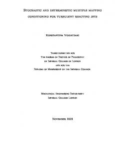
I. I NTRODUCTION Fig. 1. Random realizations of ad hoc networks in a square domain of side L = 10, using β = 1 and η = 2, 4, 6, ∞, as defined in the pair connectedness function H(r). Different connected components are shown in different colors.

Recent advancements in micro and nano-scale electronics along with the development of efficient routing protocols have rendered current wireless technologies ideal for ad hoc and sensing applications [1]. Making use of low complexity multihop relaying techniques and signal processing capabilities, sensor networks can often achieve very good coverage and connectivity over large areas, “on the fly” in a decentralized and distributed manner by self-organising into a mesh network, assigned with some data collection and dissemination task [2]. The spontaneous self-organization trait of large scale sensor networks has attracted much research attention in recent years, with particular interest in enhancing the connectivity properties of the underlying communication graph [3]. Of practical interest for example is the ability to predict the optimal number of nodes necessary to maintain good connectivity [4], or conversely, to predict the optimal average transmission range for a given number of nodes. These predictions are essential network design recommendations which can in turn act as inputs for cognitive scheduling and routing protocol selection. Furthermore, improvement in the connectivity properties of the network can have a significant impact on the operational lifetime of ad hoc sensor networks by conserving energy, and

can also improve the overall functionality, reliability and faulttolerance of the network. The analysis and resolution of network connectivity is typically addressed from a physical layer’s point of view through the theory of stochastic geometry [5], random geometric graphs [6] and complex networks [7], equipped with a plethora of methods and metrics e.g. clustering and modularity statistics, node importance, correlations between degrees of neighbouring nodes, etcetera. From a communications perspective, a popular and well studied observable of random networks is that of full connectivity [8]. This characterizes the probability Pf c with which a random realization of an ad hoc network will consist of a single connected component (cluster). Consequently, every node in the network can communicate with any other node in a multi-hop fashion. In the theory of random geometric networks, two nodes are said to connect and form a pair if they are within a certain distance r0 from each other. This is referred to as the 1

V ⊂ Rd with volume V . The node position coordinates are given by ri ∈ V for i = 1 . . . N . We say that a communication link between a pair of nodes i and j exists with probability H(rij ), where rij = |ri − rj | is the relative distance between the pair. One physical interpretation of a communication link is given by the complement of the information outage probability between two nodes for a given rate x in bits per complex dimension, which can be written as
Pr log2 (1 + SNR × |h|2 ) > x [11], where h is the channel −η transfer coefficient, and SNR ∝ rij is the average received signal to noise ratio and η is the path loss exponent. Typically η = 2 corresponds to propagation in free space but for cluttered environments it is observed to be η ≥ 2. We consider the case where the individual channel fading distributions follow a Rayleigh fading model, and all channels are statistically independent. It follows that |h|2 has a standard exponential distribution for a single-input single-output (SISO) antenna system. Hence, the connection probability H(r) between two nodes a distance r apart can be expressed as

geometric disk model and is only sufficient when modelling deterministic, distance-dependent wireless channels. One extension of this connectivity model, is to account for the channel randomness due to shadow fading and multipath effects in the spatial domain by ‘softening’ the position dependence of the pair connectedness function such that links are established in probability space [9]. In static wireless networks, this softening can be understood as modelling the randomness in the received signal power [10]. Thus, in the absence of internode interference, two nodes connect with a probability H(r) which decays as a function of the distance r between the pair. What this effectively means is that nodes which are closer than a distance r0 from each other may no longer be connected, and nodes that are more than r0 apart may be connected. The overall effect of channel randomness is typically encoded into the path loss exponent η (defined later) [11] and has been argued to have a negative effect on local connectivity, but a positive effect on overall connectivity [12]. The latter conclusion has been reached through a combination of theoretical and numerical results, the former mainly relying on the bound Pf c ≤ Pmd , where Pmd characterizes the probability with which a random realization of an ad hoc network has minimum network degree equal to one i.e. each node is connected to at least one other node. The bound was proven to be tight by Penrose in 1999 for the deterministic geometric disk model in the limit of number of nodes N → ∞ [13]. Since then, a number of papers have followed suit extending these results in many directions to include for, inter alia, boundary effects, channel randomness, and anisotropic radiation patterns. In this paper, we challenge the negative effect of channel randomness on local connectivity and also investigate the tightness of the bound Pf c ≤ Pmd for finite yet sufficiently large N and examine the role of channel randomness to this respect. We show analytically that Rayleigh fading improves local connectivity when η is less than the effective spatial dimension d of the network. We also show that the pair isolation probability Π is what distinguishes Pmd from Pf c at high node densities, and calculate closed form expressions for it assuming a Rayleigh fading channel. Both of our results are validated through extensive numerical simulations, the latter suggesting that two nodes are more likely to form an isolated pair when η is large i.e. in heavily cluttered environments. Finally, we discuss the engineering insight provided by our analysis towards facilitating the design of wireless ad hoc sensor and mesh networks [14]. The paper is structured as follows: Sec. II describes the system model and relevant assumptions. Secs. III and IV discuss local and global network observables respectively and their sensitivity to stochastic/deterministic wireless channels. Sec. V investigates analytically the pair isolation probability, and Sec. VI numerically confirms our theoretical predictions which are then summarised and discussed in Sec. VII.

η

H(r) = e−βr ,

(1)

where β sets the characteristic connection length r0 = β −1/η . Therefore, our system model has two sources of randomness: random node positions, and random link formation according to the ‘softness’ of the channel fading model controlled here by η. It is important to note that in the limit of η → ∞, the connection between nodes is no longer probabilistic and converges to the geometric disk model, with an on/off connection range at the limiting r0 . We will later make use of this limit in order to compare the connectivity of random networks using deterministic or stochastic point-to-point link models. Fig. 1 shows how N = 150 nodes scattered randomly in a square domain of side L = 10, connect to form different networks for different values of η = 2, 4, 6, and ∞, using β = 1. The corresponding H(r) functions are also plotted below each panel in order to give the reader a feeling of how probable shorter and longer than r0 links are in the presence of Rayleigh fading. We stress that in practice, an efficient medium access control (MAC) layer protocol is typically required e.g. using a Time Division Multiple Access (TDMA) scheme in order to render inter-node interference negligible. Alternatively, a low traffic network may be assumed so that the communication network can be modelled as seen in Fig. 1. III. L OCAL C ONNECTIVITY AND M EAN D EGREE The network mean degree µ is a local observable of network connectivity characterising the average number of one-hop neighbours of a typical node. For random geometric networks as R described in Sec. II, this can be expressed as H(rij )dri drj which follows from multiplying µ = NV−1 2 V2 N −1 by the probability of two randomly selected nodes (i and j) connecting to form a pair. Assuming that V is large and the typical length scale of the domain is greater than the effective connection range r0 , a typical node is most likely to be found away from the borders of the domain. Moreover, since H(r) is decaying exponentially, it is reasonable to expect that the

II. S YSTEM M ODEL We consider a network of N nodes distributed randomly and uniformly in a d = 2, 3, dimensional convex domain 2

a wireless link to at least one access point, in decentralized ad hoc networks, efficient routing protocols can utilize mutually independent paths to communicate information through the network e.g. for sensing, monitoring, alerting or storage purposes [1]. Therefore, if a multihop path exists between all pairs of nodes, then the network is fully connected and in a sense is both delay and disruption tolerant [15]. A generalization of the concept of full connectivity is that of k−connectivity [16]. A fully connected network is said to be k-connected if the removal of any k − 1 nodes leaves the remaining network fully connected. The removal of nodes may model technical failures (e.g. a hardware/software malfunction) or attacks which can disrupt the functionality and operation of the network, in some cases leading to cascades of catastrophic failures [17]. Equivalently, k-connectivity also guarantees that for each pair of nodes there exist at least k mutually independent paths connecting them [6]. Therefore, k-connectivity is an important measure of network robustness, resilience but also of routing diversity. It is clear that a k-connected network has minimum degree k, i.e. each node has at least k neighbouring nodes. The opposite statement is not true however and hence the former set is a subset of the latter and so Pf c (k) ≤ Pmd (k), where Pf c (k) denotes the probability that a random realization of an ad hoc network is k-connected, and Pmd (k) denotes the probability that it has minimum degree k. These two observables are however strongly related through a fundamental concept originally proven in [13] (Theorem 1.1) which states that “if N is big enough, then with high probability, if one starts with isolated points and then adds edges connecting the points in order of increasing separation length, then the resulting graph becomes k-connected at the instant when it achieves a minimum degree of k”. Ever since this realization, Pf c (k) has been approximated by Pmd (k) [18] as it is easier to express mathematically, and evaluate numerically. Specifically, we have that [16]

Fig. 2. Plot of the mean degree µ as a function of η, obtained from numerical simulations of ad hoc networks in a square of side L = 10 (blue), and a cube of side L = 7 (purple). In both cases β = ρ = 1. The analytical predictions of (2) are shown as solid curves and the limit µ∞ as dashed lines.

degree of a typical node is very much insensitive to boundary effects, thus justifying the following approximation Z Z ∞ ΩΓ( ηd ) η (2) µη ≈ ρ H(r)dr = ρ Ω rd−1 e−βr dr = ρ d Rd 0 ηβ η d

2π 2 is the solid angle in d dimenwhere ρ ≈ NV−1 and Ω = Γ( d 2) sions. In (2) we have effectively assumed that the network is homogeneous i.e. it is translation and rotation invariant, such that we can set ri = 0 and extend the radial integral of rj to infinity taking on exponentially small errors. Substituting β = r0−η and taking the limit η → ∞ we obtain an expression for the mean degree for the deterministic geometric disk rd model µ∞ = ρ Ω d0 . Comparing this to the result of (2), we conclude that µ∞ = µη when η = d and that µη < µ∞ for η > d. In other words, the stochastic and deterministic connectivity models are equivalent at η = d when viewed locally. More importantly however, Rayleigh fading reduces the local network connectivity when η > d, but improves it when η < d. The latter condition describes a very special case when the network resides in an effectively 2D plane, but may well be significant in 3D networks deployed in multi-storey buildings for example where the path loss exponent may be in the range 2 ≤ η < 3. Consequently, one may significantly over or under specify network design features and deployment methods if the network is not correctly modelled. Numerical verification of the above result is presented in Fig. 2 showing computer Monte Carlo simulations of ad hoc networks in two and three dimensions. The analytical predication of (2) and the limit case of µ∞ are also shown for comparison. An almost perfect agreement is observed between theory and simulations with the theoretical result typically being smaller than the numerical one. This is because µη was approximated assuming no boundary effects, which hinder connectivity for nodes near the borders of V. The minimum value of µη is obtained numerically at η ≈ 4.33 and η ≈ 6.50 in two and three dimensional networks respectively. We now turn to investigate global network observables.

Pmd (k) = h

N Y

P (degree(ri ) ≥ k)i

i=1

#N (3) Z ρm 1 m MH (ri )e−ρMH (ri ) dri , ≈ 1− m! V V m=0 R where MH (ri )= V H(rij )drj and V is assumed to be much larger than πr0d . The angled brackets in (3) represent a spatial average of a network observable O over all possible node configurations and is defined as Z 1 hOi = N O(r1 , r2 , . . . , rN )dr1 dr2 . . . drN . (4) V VN "

k−1 X

We will use this notation in order to calculate expectation values of different random network observables. Fig. 3 shows Monte Carlo computer simulations for η = 2 (left panels) and η = ∞ (right panels). 105 random networks were simulated in a square domain of side L = 10 for a range of node density values ρ ∈ (1, 8) using β = 1, in order to obtain curves for Pf c (k) and Pmd (k) for k = 1, 2, 3, and 4.

IV. k-C ONNECTIVITY AND M INIMUM D EGREE In the absence of a fixed infrastructure (e.g. cellular, or WLANs), where it is sufficient that each network node has 3

Using the spatial average defined in (4), and letting Hij = H(rij ) in order to save space, we write X Y Π(1) = h Hij (1 − Hik )(1 − Hjk )i i