problems in Chapter 3. We now return to the formulation of these models, and
AMPL's features for handling them. Figure 15-1 shows the sort of diagram ...
Copyright © 2003 by Robert Fourer, David M. Gay and Brian W. Kernighan
15
________________________ ________________________________________________________________________
Network Linear Programs Models of networks have appeared in several chapters, notably in the transportation problems in Chapter 3. We now return to the formulation of these models, and AMPL’s features for handling them. Figure 15-1 shows the sort of diagram commonly used to describe a network problem. A circle represents a node of the network, and an arrow denotes an arc running from one node to another. A flow of some kind travels from node to node along the arcs, in the directions of the arrows. An endless variety of models involve optimization over such networks. Many cannot be expressed in any straightforward algebraic way or are very difficult to solve. Our discussion starts with a particular class of network optimization models in which the decision variables represent the amounts of flow on the arcs, and the constraints are limited to two kinds: simple bounds on the flows, and conservation of flow at the nodes. Models restricted in this way give rise to the problems known as network linear programs. They are especially easy to describe and solve, yet are widely applicable. Some of their benefits extend to certain generalizations of the network flow form, which we also touch upon. We begin with minimum-cost transshipment models, which are the largest and most intuitive source of network linear programs, and then proceed to other well-known cases: maximum flow, shortest path, transportation and assignment models. Examples are initially given in terms of standard AMPL variables and constraints, defined in var and subject to declarations. In later sections, we introduce node and arc declarations that permit models to be described more directly in terms of their network structure. The last section discusses formulating network models so that the resulting linear programs can be solved most efficiently.
15.1 Minimum-cost transshipment models As a concrete example, imagine that the nodes and arcs in Figure 15-1 represent cities and intercity transportation links. A manufacturing plant at the city marked PITT will
319
320
NETWORK LINEAR PROGRAMS
CHAPTER 15
________________________________________________________________________ ____________________________________________________________________________________________________________________________________________________________________________________
BOS 90 1.7, 100 0.7, 100
NE
EWR 120
2.5, 250 1.3, 100 450 PITT
BWI 120 1.3, 100 3.5, 250
0.8, 100 SE
0.2, 100
ATL 70
2.1, 100 MCO 50
Figure 15-1: A directed network. ________________________________________________________________________ ____________________________________________________________________________________________________________________________________________________________________________________
make 450,000 packages of a certain product in the next week, as indicated by the 450 at the left of the diagram. The cities marked NE and SE are the northeast and southeast distribution centers, which receive packages from the plant and transship them to warehouses at the cities coded as BOS, EWR, BWI, ATL and MCO. (Frequent flyers will recognize Boston, Newark, Baltimore, Atlanta, and Orlando.) These warehouses require 90, 120, 120, 70 and 50 thousand packages, respectively, as indicated by the numbers at the right. For each intercity link there is a shipping cost per thousand packages and an upper limit on the packages that can be shipped, indicated by the two numbers next to the corresponding arrow in the diagram. The optimization problem over this network is to find the lowest-cost plan of shipments that uses only the available links, respects the specified capacities, and meets the requirements at the warehouses. We first model this as a general network flow problem, and then consider alternatives that specialize the model to the particular situation at hand. We conclude by introducing a few of the most common variations on the network flow constraints.
A general transshipment model To write a model for any problem of shipments from city to city, we can start by defining a set of cities and a set of links. Each link is in turn defined by a start city and an end city, so we want the set of links to be a subset of the set of ordered pairs of cities: set CITIES; set LINKS within (CITIES cross CITIES);
SECTION 15.1
MINIMUM-COST TRANSSHIPMENT MODELS
321
Corresponding to each city there is potentially a supply of packages and a demand for packages: param supply {CITIES} >= 0; param demand {CITIES} >= 0;
In the case of the problem described by Figure 15-1, the only nonzero value of supply should be the one for PITT, where packages are manufactured and supplied to the distribution network. The only nonzero values of demand should be those corresponding to the five warehouses. The costs and capacities are indexed over the links: param cost {LINKS} >= 0; param capacity {LINKS} >= 0;
as are the decision variables, which represent the amounts to ship over the links. These variables are nonnegative and bounded by the capacities: var Ship {(i,j) in LINKS} >= 0, = 0; param demand {CITIES} >= 0;
# amounts available at cities # amounts required at cities
check: sum {i in CITIES} supply[i] = sum {j in CITIES} demand[j]; param cost {LINKS} >= 0; param capacity {LINKS} >= 0;
# shipment costs/1000 packages # max packages that can be shipped
var Ship {(i,j) in LINKS} >= 0, = 0; param w_demand {W_CITY} >= 0;
These declarations allow supply and demand to be defined only where they belong. At this juncture, we can define the sets CITIES and LINKS and the parameters supply and demand as they would be required by our previous model: set CITIES = {p_city} union D_CITY union W_CITY; set LINKS = ({p_city} cross D_CITY) union DW_LINKS; param supply {k in CITIES} = if k = p_city then p_supply else 0; param demand {k in CITIES} = if k in W_CITY then w_demand[k] else 0;
The rest of the model can then be exactly as in the general case, as indicated in Figures 15-3a and 15-3b.
324
NETWORK LINEAR PROGRAMS
CHAPTER 15
________________________________________________________________________ ____________________________________________________________________________________________________________________________________________________________________________________
param p_city symbolic; set D_CITY; set W_CITY; set DW_LINKS within (D_CITY cross W_CITY); param p_supply >= 0; param w_demand {W_CITY} >= 0;
# amount available at plant # amounts required at warehouses
check: p_supply = sum {k in W_CITY} w_demand[k]; set CITIES = {p_city} union D_CITY union W_CITY; set LINKS = ({p_city} cross D_CITY) union DW_LINKS; param supply {k in CITIES} = if k = p_city then p_supply else 0; param demand {k in CITIES} = if k in W_CITY then w_demand[k] else 0; ### Remainder same as general transshipment model ### param cost {LINKS} >= 0; param capacity {LINKS} >= 0;
# shipment costs/1000 packages # max packages that can be shipped
var Ship {(i,j) in LINKS} >= 0, = 0; param dw_cost {DW_LINKS} >= 0; param pd_cap {D_CITY} >= 0; param dw_cap {DW_LINKS} >= 0; var PD_Ship {i in D_CITY} >= 0, = 0, = 0; param w_demand {W_CITY} >= 0;
# amount available at plant # amounts required at warehouses
check: p_supply = sum {j in W_CITY} w_demand[j]; param pd_cost {D_CITY} >= 0; param dw_cost {DW_LINKS} >= 0;
# shipment costs/1000 packages
param pd_cap {D_CITY} >= 0; param dw_cap {DW_LINKS} >= 0;
# max packages that can be shipped
var PD_Ship {i in D_CITY} >= 0, = 0, 0;
Then the demand constraints at the warehouses are adjusted as follows: subject to W_Bal {j in W_CITY}: sum {(i,j) in DW_LINKS} (1000/ppc) * DW_Ship[i,j] = w_demand[j];
The term (1000/ppc) * DW_Ship[i,j] represents the number of cartons received at warehouse j when DW_Ship[i,j] thousand packages are shipped from distribution center i.
328
NETWORK LINEAR PROGRAMS
CHAPTER 15
________________________________________________________________________ ____________________________________________________________________________________________________________________________________________________________________________________
a
50
b 20
100
40
c
60
50
d
e
60
20
f
70 70
g
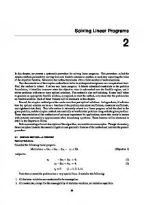
Figure 15-5: Traffic flow network. ________________________________________________________________________ ____________________________________________________________________________________________________________________________________________________________________________________
15.2 Other network models Not all network linear programs involve the transportation of things or the minimization of costs. We describe here three well-known model classes — maximum flow, shortest path, and transportation/assignment — that use the same kinds of variables and constraints for different purposes. Maximum flow models In some network design applications the concern is to send as much flow as possible through the network, rather than to send flow at lowest cost. This alternative is readily handled by dropping the balance constraints at the origins and destinations of flow, while substituting an objective that stands for total flow in some sense. As a specific example, Figure 15-5 presents a diagram of a simple traffic network. The nodes and arcs represent intersections and roads; capacities, shown as numbers next to the roads, are in cars per hour. We want to find the maximum traffic flow that can enter the network at a and leave at g. A model for this situation begins with a set of intersections, and symbolic parameters to indicate the intersections that serve as entrance and exit to the road network: set INTER; param entr symbolic in INTER; param exit symbolic in INTER, entr;
The set of roads is defined as a subset of the pairs of intersections: set ROADS within (INTER diff {exit}) cross (INTER diff {entr});
This definition ensures that no road begins at the exit or ends at the entrance. Next, the capacity and traffic load are defined for each road:
SECTION 15.2
OTHER NETWORK MODELS
329
________________________________________________________________________ ____________________________________________________________________________________________________________________________________________________________________________________
set INTER;
# intersections
param entr symbolic in INTER; param exit symbolic in INTER, entr;
# entrance to road network # exit from road network
set ROADS within (INTER diff {exit}) cross (INTER diff {entr}); param cap {ROADS} >= 0; var Traff {(i,j) in ROADS} >= 0, = 0; var Traff {(i,j) in ROADS} >= 0, = 0; var Use {(i,j) in ROADS} >= 0;
# times to travel roads # 1 iff (i,j) in shortest path
minimize Total_Time: sum {(i,j) in ROADS} time[i,j] * Use[i,j];
Since only those variables Use[i,j] on the optimal path equal 1, while the rest are 0, this sum does correctly represent the total time to traverse the optimal path. The only other change is the addition of a constraint to ensure that exactly one unit of flow is available at the entrance to the network: subject to Start:
sum {(entr,j) in ROADS} Use[entr,j] = 1;
The complete model is shown in Figure 15-7. If we imagine that the numbers on the arcs in Figure 15-5 are travel times in minutes rather than capacities, the data are the same; AMPL finds the solution as follows: ampl: model netshort.mod; ampl: solve; MINOS 5.5: optimal solution found. 1 iterations, objective 140 ampl: option omit_zero_rows 1; ampl: display Use; Use := a b 1 b e 1 e g 1 ;
The shortest path is a → b → e → g, which takes 140 minutes. Transportation and assignment models The best known and most widely used special network structure is the ‘‘bipartite’’ structure depicted in Figure 15-8. The nodes fall into two groups, one serving as origins of flow and the other as destinations. Each arc connects an origin to a destination.
SECTION 15.2
OTHER NETWORK MODELS
331
________________________________________________________________________ ____________________________________________________________________________________________________________________________________________________________________________________
set INTER;
# intersections
param entr symbolic in INTER; param exit symbolic in INTER, entr;
# entrance to road network # exit from road network
set ROADS within (INTER diff {exit}) cross (INTER diff {entr}); param time {ROADS} >= 0; var Use {(i,j) in ROADS} >= 0;
# times to travel roads # 1 iff (i,j) in shortest path
minimize Total_Time: sum {(i,j) in ROADS} time[i,j] * Use[i,j]; subject to Start:
sum {(entr,j) in ROADS} Use[entr,j] = 1;
subject to Balance {k in INTER diff {entr,exit}}: sum {(i,k) in ROADS} Use[i,k] = sum {(k,j) in ROADS} Use[k,j]; data; set INTER := a b c d e f g ; param entr := a ; param exit := g ; param:
ROADS: a b b d c d d e e g
time := 50, a c 40, b e 60, c f 50, d f 70, f g
100 20 20 60 70 ;
Figure 15-7: Shortest path model and data (netshort.mod). ________________________________________________________________________ ____________________________________________________________________________________________________________________________________________________________________________________
The minimum-cost transshipment model on this network is known as the transportation model. The special case in which every origin is connected to every destination was introduced in Chapter 3; an AMPL model and sample data are shown in Figures 3-1a and 3-1b. A more general example analogous to the models developed earlier in this chapter, where a set LINKS specifies the arcs of the network, appears in Figures 6-2a and 6-2b. Every path from an origin to a destination in a bipartite network consists of one arc. Or, to say the same thing another way, the optimal flow along an arc of the transportation model gives the actual amount shipped from some origin to some destination. This property permits the transportation model to be viewed alternatively as a so-called assignment model, in which the optimal flow along an arc is the amount of something from the origin that is assigned to the destination. The meaning of assignment in this context can be broadly construed, and in particular need not involve a shipment in any sense. One of the more common applications of the assignment model is matching people to appropriate targets, such as jobs, offices or even other people. Each origin node is associated with one person, and each destination node with one of the targets — for example, with one project. The sets might then be defined as follows: set PEOPLE; set PROJECTS; set ABILITIES within (PEOPLE cross PROJECTS);
332
NETWORK LINEAR PROGRAMS
CHAPTER 15
________________________________________________________________________ ____________________________________________________________________________________________________________________________________________________________________________________
DET
FRA CLEV FRE
GARY
LAF
LAN PITT STL
WIN
Figure 15-8: Bipartite network. ________________________________________________________________________ ____________________________________________________________________________________________________________________________________________________________________________________
The set ABILITIES takes the role of LINKS in our earlier models; a pair (i,j) is placed in this set if and only if person i can work on project j. As one possibility for continuing the model, the supply at node i could be the number of hours that person i is available to work, and the demand at node j could be the number of hours required for project j. Variables Assign[i,j] would represent the number of hours of person i’s time assigned to project j. Also associated with each pair (i,j) would be a cost per hour, and a maximum number of hours that person i could contribute to job j. The resulting model is shown in Figure 15-9. Another possibility is to make the assignment in terms of people rather than hours. The supply at every node i is 1 (person), and the demand at node j is the number of people required for project j. The supply constraints ensure that Assign[i,j] is not greater than 1; and it will equal 1 in an optimal solution if and only if person i is assigned to project j. The coefficient cost[i,j] could be some kind of cost of assigning person i to project j, in which case the objective would still be to minimize total cost. Or the coefficient could be the ranking of person i for project j, perhaps on a scale from 1 (highest) to 10 (lowest). Then the model would produce an assignment for which the total of the rankings is the best possible. Finally, we can imagine an assignment model in which the demand at each node j is also 1; the problem is then to match people to projects. In the objective, cost[i,j] could be the number of hours that person i would need to complete project j, in which case the model would find the assignment that minimizes the total hours of work needed to finish all the projects. You can create a model of this kind by replacing all references
SECTION 15.3
DECLARING NETWORK MODELS BY NODE AND ARC
333
________________________________________________________________________ ____________________________________________________________________________________________________________________________________________________________________________________
set PEOPLE; set PROJECTS; set ABILITIES within (PEOPLE cross PROJECTS); param supply {PEOPLE} >= 0; # hours each person is available param demand {PROJECTS} >= 0; # hours each project requires check: sum {i in PEOPLE} supply[i] = sum {j in PROJECTS} demand[j]; param cost {ABILITIES} >= 0; param limit {ABILITIES} >= 0;
# cost per hour of work # maximum contributions to projects
var Assign {(i,j) in ABILITIES} >= 0, = 0, = 0; param demand {CITIES} >= 0;
# amounts available at cities # amounts required at cities
check: sum {i in CITIES} supply[i] = sum {j in CITIES} demand[j]; param cost {LINKS} >= 0; param capacity {LINKS} >= 0;
# shipment costs/1000 packages # max packages that can be shipped
minimize Total_Cost; node Balance {k in CITIES}: net_in = demand[k] - supply[k]; arc Ship {(i,j) in LINKS} >= 0, = 0; param w_demand {W_CITY} >= 0;
# amount available at plant # amounts required at warehouses
check: p_supply = sum {j in W_CITY} w_demand[j]; param pd_cost {D_CITY} >= 0; # shipment costs/1000 packages param dw_cost {DW_LINKS} >= 0; param pd_cap {D_CITY} >= 0; param dw_cap {DW_LINKS} >= 0;
# max packages that can be shipped
minimize Total_Cost; node Plant: net_out = p_supply; node Dist {i in D_CITY}; node Whse {j in W_CITY}: net_in = w_demand[j]; arc PD_Ship {i in D_CITY} >= 0, = 0, = 0, = 0, = 0; node Intersection {k in INTER diff {entr,exit}};
The condition net_out >= 0 implies that the flow out of node Entr_Int may be any amount at all; this is the proper condition, since there is no balance constraint on the entrance node. An analogous comment applies to the condition for node Exit_Int. There is one arc in this network for each pair (i,j) in the set ROADS. Thus the declaration should look something like this: arc Traff {(i,j) in ROADS} >= 0, = 0, = 0, = 0, from Intersection[exit]; arc Traff {(i,j) in ROADS} >= 0, = 0, to Intersection[entr]; arc Traff_Out >= 0, from Intersection[exit];
The arcs that represent roads within the network are declared as before: arc Traff {(i,j) in ROADS} >= 0, =
SECTION 15.4
RULES FOR NODE AND ARC DECLARATIONS
341
and = 0; param demand {CITIES,PRODS} >= 0;
# amounts available at cities # amounts required at cities
check {p in PRODS}: sum {i in CITIES} supply[i,p] = sum {j in CITIES} demand[j,p]; param cost {LINKS,PRODS} >= 0; # shipment costs/1000 packages param capacity {LINKS,PRODS} >= 0; # max packages shipped param cap_joint {LINKS} >= 0; # max total packages shipped/link minimize Total_Cost; node Balance {k in CITIES, p in PRODS}: net_in = demand[k,p] - supply[k,p]; arc Ship {(i,j) in LINKS, p in PRODS} >= 0, = 0;
We imagine that at city k, in addition to the amounts supply[p,k] of products available to be shipped, up to limit[f,k] of feedstock f can be converted into products; one unit of feedstock f gives rise to yield[p,f] units of each product p. A variable Feed[f,k] represents the amount of feedstock f used at city k: var Feed {f in FEEDS, k in CITIES} >= 0, = 0;
# amounts available at cities
param demand {PRODS,CITIES} >= 0;
# amounts required at cities
check {p in PRODS}: sum {i in CITIES} supply[p,i] = sum {j in CITIES} demand[p,j]; param cost {PRODS,LINKS} >= 0; # shipment costs/1000 packages param capacity {PRODS,LINKS} >= 0; # max packages shipped of product set FEEDS; param yield {PRODS,FEEDS} >= 0; param limit {FEEDS,CITIES} >= 0;
# amounts derived from feedstocks # feedstocks available at cities
minimize Total_Cost; var Feed {f in FEEDS, k in CITIES} >= 0, = 0, = 0; param link_cap {LINKS} >= 0;
The arc capacities represent, as before, upper limits on the shipments between cities. The node capacities limit the throughput, or total flow handled at a city, which may be written as the supply at the city plus the sum of the flows in, or equivalently as the demand at the city plus the sum of the flows out. Using the former, we arrive at the following constraint: subject to through_limit {k in CITIES}: supply[k] + sum {(i,k) in LINKS} Ship[i,k] = 0; param demand {CITIES} >= 0;
# amounts available at cities # amounts required at cities
check: sum {i in CITIES} supply[i] = sum {j in CITIES} demand[j]; param cost {LINKS} >= 0;
# shipment costs per ton
param city_cap {CITIES} >= 0; # max throughput at cities param link_cap {LINKS} >= 0; # max shipment over links minimize Total_Cost; node Supply {k in CITIES}: net_out = supply[k]; node Demand {k in CITIES}: net_in = demand[k]; arc Ship {(i,j) in LINKS} >= 0, = 0, = 0, = 0,