Network Models and Archaeological Spaces

th

27 July 2011

Network Models and Archaeological Spaces Ray Rivers, Department of Physics, Imperial College London, SW7 2AZ, UK Carl Knappett, Department of Art, University of Toronto, Canada Tim S. Evans, Department of Physics, Imperial College London, SW7 2AZ, UK Contribution to “Computational Approaches to Archaeological Spaces” eds A.Bevan, M.Lake Contents

I. Introduction II. The Role of Geographic Space: First Thoughts   

A question of „distance‟: Fixed radius model (Ariadne VP) Proximal Point Analysis (Ariadne PPA) Agency: Optimisation

III. The ‘Most Likely’ Networks 

Maximum entropy: Basic gravity models



Rihll and Wilson model (Ariadne RW)

IV. The ‘Most Efficient’ Networks  

Utility functions or social potentials (Ariadne MC) Is almost the best good enough?

V. Does It Work? VI. Summary References

I.

Introduction

A fundamental ingredient of archaeological analysis is an understanding of spatial relationships. We concur with Renfrew (Renfrew 1981, p268) that “the very activity of examining the spatial correlates of early social structure has the useful effect of posing important problems in general and simple terms”. Posed as generally as this, it is not altogether surprising that different authors have provided almost as many answers as there are questions and to shape the discussion which follows we have chosen to put a heavy emphasis upon the Bronze Age Aegean, the period for which our own models (Knappett et al. 2008; 2011; Evans et al. 2009) of maritime trade and exchange routes were devised. This is because the act of constructing and developing them has illuminated problems common to many approaches. The original focus of our work was the southern Aegean in the Middle (MBA) and early Late Bronze Age. This is well bounded in time, concluding with the „burning of the palaces‟ some time after the eruption of Thera. The archaeological record poses some interesting questions. On the one hand, we wanted to understand why some sites, like Knossos on Crete, grew to be so large and influential. On the other hand, we wanted to understand how the volcanic eruption of Thera seemed to have such little immediate effect on the exchange between Minoan Crete and the surrounding regions despite destroying Akrotiri, which might have been anticipated as the main gateway from Knossos into the Cyclades, Peloponnese and the Greek mainland. Although both address spatial issues, superficially these questions seem very different. Thus, the emergence and characteristics of sites like Knossos are partially explained in local terms, with these local conditions only then facilitating exchange with other sites. The global stability of the Minoan exchange network, meanwhile, might be thought of as explicable in terms of Aegean geography and marine technology, since the appearance of the sail from about 2000 BC facilitated new levels of inter-regional interaction. However, to separate local power from global organisation too strongly is to set up a false dichotomy, since the centres of local power are also likely to be key players in global exchange. The same routes that enable these centres to maintain their influence are also conduits for the entwined cultural and economic connections between them. As a result, their growth and importance will be conditioned by the characteristics of the larger networks to which they belong, leading to what Batty terms an „archaeology of relations‟ (Batty 2005, p149). In our Aegean work we have argued that network models can provide the natural framework to transcend this dualism between physical and relational space. Networks are, in essence, no more than a set of nodes or vertices connected by links or edges. Most simply, in archaeology we identify nodes with archaeological sites and the communities that inhabited these sites, and links with the exchange between them. Networks thus have the potential, in an almost selfevident way, of encoding „spatial correlates‟ by incorporating both the local attributes of sites together with their global interactions and showing the reciprocal effect of the one on the other. It is no surprise that island archipelagos lend themselves to network analysis. With a dominant means of interaction (sea travel) and, typically, a dominant sailing technology (canoe or sailing vessels) they allow for simple connectivity. In this article we are primarily interested in how networks of relationships are conditioned by what, in shorthand, we might term ‟geographical space‟. In the next section we give an overview of some of the issues that arise in constructing network models for archaeology that

rely heavily on the basic attributes of physical geography; distance and topography. Null models are useful in this, in helping to provide simple benchmarks. This prefigures the most substantive part of the Chapter, an analysis of how „optimisation‟ models, which add „agency‟ to „geography‟, might be useful in Aegean prehistory. Although such modelling has obvious limitations, in its stress on the material circumstances of human-environment interaction on social change, it allows for a „restricted set of spatial variables to play a role in shaping historical transformations‟, (Smith, 2003, p53). As a result, in a step by step way, we can construct tractable quantitative models amenable to simulation. In trying to decide whether and how such models „work‟, it is hard to improve upon the sentiment in Rihll and Wilson (Rihll and Wilson 1991, p62) that “The purpose of a good model is to formulate simple concepts and hypotheses concerning them, and to demonstrate that, despite their simplicity, they give approximate accounts of otherwise complex behaviour of phenomena. If a model „works‟ (faithfully represents the known evidence) then it shows that the assumptions and hypotheses built into the model contribute to an explanation of the phenomena” Unfortunately, although the „evidence‟, the archaeological record, may be good for some eras, for the prehistoric era of our models it is sufficiently patchy in both space and time as to be ambiguous. If the data sets were good, whether the model could be made to „work‟ would become apparent quite quickly. Unfortunately, with the data as incomplete as it is, we might expect to find so many choices of model to be commensurate with the data that it would not be clear how to proceed. In practice, this is not the case. A simple touchstone is that the models should produce a range of site occupancies and a range of site activity that go beyond the range of potential resources. Despite this seeming generality we stress that there is no universal behaviour implied by network models and this alone turns out to be a surprisingly good discriminant. Different models give different patterns of exchange and we need to choose the model type appropriately, with even a poor record in mind, before we look further at the detailed behaviour that they can suggest. This, in turn, requires further assumptions about (marine) technology and social organization specific to the period in question. There are then yet further issues about determinacy, and to what extent we should understand outcomes statistically, that we shall do our best to address in the space at our disposal. Although motivated by the MBA S. Aegean, this article is more an overview of methods and we shall not attempt to address the archaeological record in detail. Steps towards this are given elsewhere (Knappett et al. 2011). .

II.

The Role of Geographic Space: First Thoughts

One attribute common to most network models is that they are construed dynamically. Links describe the flows between sites; goods, raw materials, people, ideas, both the sinews and synapses of inter-site relationships. In the most simple networks, links are non-directional and either switched on or off, i.e. all we are concerned with is whether two sites interact or not. At a more sophisticated level, links are both directional (i.e. the relationship of A to B is not the same as B to A) and are „weighted‟ (i.e. vary from strong to weak, where the weight is a measure of the „flow‟). In an archaeological context nodes, thought of as sites, have two different attributes. At one level we can interpret them as junctions for flows, without needing any of their local physical and

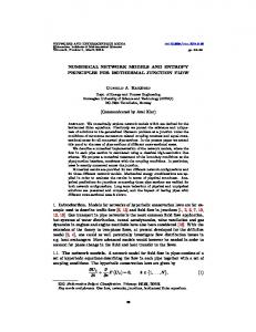
geographical properties beyond, say, position, which determines their accessibility to other sites. In this sense they are rather like traffic intersections, or airports, only acquiring their local significance from the network as a whole. This permits a variety of classifications, of which the simplest orders nodes by their „busyness‟, the total flow through them. However, we should not ignore their local properties. In fact, our original interest in networks was triggered by the use of networks to explain the mismatch between local resources and exchange in the Early Bronze Age Cyclades (Broodbank 2000). In some models (our first null models) sites are treated equally but, more realistically, are ranked by their local properties (e.g. populations) as well as their properties derived from the global behaviour of the network as a whole. As we said earlier, our main interest is to see to what extent exchange networks reflect or transcend what we have termed geographical space. Such „space‟ has several facets, which we shall delineate later but, as a first guess, by looking at the site map, could we infer which sites are most significant, both from their intrinsic properties (e.g. resources) and their position in the network? We also need to identify the most important links since they will reflect the distribution of artefacts. We begin this discussion by presenting two null models, each of which uses only physical geography, qualified by basic assumptions about travel, against which to test the more sophisticated hypotheses that we shall propose later. A question of ‘distance’: Fixed radius model The map of the S. Aegean whose networks we are considering is given in Fig.1. On it we have labelled 39 of the most significant sites in the MBA. Names and details of the sites are given in the Appendix in Table 1. In general we do not need them, since we are mainly using the resulting networks for comparative purposes, and will not address the record in any detail. In the first instance, what we see is four regional groupings; Crete, the Cyclades, the Peloponnese and the Dodecanese. One of the tests for the importance of geography lies in the extent to which the exchange networks reflect these regional groupings. To convert these qualitative regional groupings into something more quantitative we have shown a dendrogram of site separations in Fig.2. However, it would have been too simplistic to have constructed it with a compass, using just geographical distances. For exchange networks the relevant distances are those taken by the travellers who provide the exchange, which requires an understanding of how they travel. For the period in question, the MBA, communication is by sailing ships which do not remain at sea at night. Our distances are not line-of-sight distances but correspond to the best sea routes, negotiating headlands where necessary. Even that is not sufficient, since land travel may produce routes which are shorter and some sites are inland, notably Knossos and Mycenae Given the slow and laborious nature of land travel in this era, we introduce a `frictional coefficient‟ that penalises land travel over sea travel. This isolates many sites situated on large islands or on the mainland so that they behave rather like islands themselves. For instance the direct routes between some sites on the North and South coast of Crete are not optimal for reasonable friction coefficients. Sea travel round the Eastern or Western tips, or at least to a narrower part of the island, is often easier in our terms. Given our choice of optimal routes, we have used a variety of frictional coefficients and find that our conclusions are largely insensitive to them. For the sake of argument we have taken a frictional coefficient of three in all that follows. Given this relative insensitivity, our distance estimates were obtained by analysing the physical geography by hand at a scale of around a few km, an appropriate level of error given the other uncertainties in our knowledge. One of these is how, or if, to take into account the prevailing winds and currents or the daily fluctuations in conditions. For the moment we assume that these average out on a yearly cycle. Our effective distances

thus reflect averaged time-of-travel and we use the same estimates in all the models discussed below.

Fig. 1: Important sites, for the MBA Aegean, including Knossos (1) and Thera (10). The sea journey from the N. Cretan coast to Thera is a little over 100km.

1. 2. 3. 4. 5. 6. 7. 8. 9. 10. 11. 12. 13.

Knossos (L) Malia (L) Phaistos (L) Kommos (M) Ayia Triadha (L) Palaikastro (L) Zakros (M) Gournia (L) Chania (L) Thera (M) Phylakopi (M) Kastri (M) Naxos (L)

14. 15. 16. 17. 18. 19. 20. 21. 22. 23. 24. 25. 26.

Kea (M) Karpathos (S) Rhodes (L) Kos (M) Miletus (L) Iasos (M) Samos (M) Petras (L) Rethymnon (L) Paroikia (M) Amorgos (S) Ios (S) Aegina (M)

27. 28. 29. 30. 31. 32. 33. 34. 35. 36. 37. 38. 39.

Mycenae (L) Ayios Stephanos (L) Lavrion (M) Kasos (S) Kalymnos (S) Myndus (M) Cesme (M) Akbuk (M) Menelaion (S) Argos (M) Lerna (M) Asine (S) Eleusis (M)

Table 1. The sites enumerated in Fig.1 and the size of their local resource base, with (S), (M), (L) denoting „small‟, medium‟ or „large‟ respectively in terms of their resource base (input). This is to be distinguished from their „populations‟, which are outputs.

Our first model is preposterously simple. It asks what networks would occur if travel was restricted to journeys up to a specified distance, in the sense above. This is the quantitative way of defining regional clusters. In order to identify the important travel distance scales for the sites of Fig.1, the simplest way is to connect sites only if they are less than a certain distance D apart (e.g. 100km), as encoded in the dendrogram shown in Fig.2. A horizontal line at some fixed distance scale D cuts the tree into a number of smaller branches lying below the line, each defining a separate cluster of sites. Only sites within the same cluster are connected to each other by paths in which each section is less than the distance D apart. We should not think of D too precisely, both because of the uncertainty in the calculation of effective distances and because of the simplistic nature of a discrete distance cutoff. However,

in Fig.2 we see a transition occurs if we go from below 110km to above 130km (the effective distance between Knossos and Akrotiri is about 130km, once land travel is taken into account). At 110km the sites are split into the four isolated zones we would expect; Crete, the Cyclades, the Dodecanese and the Peloponnese (itself fractured into adjacent parts). On the other hand, almost all the sites are connected by routes involving steps of 130km or more. This structure becomes very clear if, as a complementary approach, we show the network for different distance scales, as in Fig.3. The dark links correspond to distances up to the specified distance.

Fig. 2: Dendrogram for the sites of Fig.1, using an effective shortest distance between sites in which sea travel is counted in physical kilometres but land travel is penalised by a `friction‟ factor of 3.0. A horizontal line cutting the vertical axis at distance scale D cuts the dendrogram into a number of disconnected branches below the horizontal line. Each of these separate branches defines a cluster (or community) of sites within which any pair of sites are separated by an effective distance of D or less. It is not possible to move between sites in different branches without following a link effective length greater than D.

Simple as this model is, one thing we take from it is the very striking fact that the distance scale D≈120km at which we move from a fragmented network to one in which can be traversed easily, albeit in several steps, is more or less the maximum distance scale we would expect from MBA sailing vessels for a single journey, on the assumption that boats did just that in travelling from the N. Cretan coast to Thera.

Figs. 3. Fixed Radius Networks for the sites of Fig.1. Sites are placed at their geographical location. Distances between sites are judged via shortest sensible routes with land travel penalised by a factor of 3.0 but without taking currents, winds etc in to account. Two sites are linked (dark links) if the effective distance is less than D, where D = 70km, 100km, 130km and 150km. Light grey links are edges which are longer than D but by no more than 20%. Sites of same colour are connected by routes via black links (i.e. all hops are less than D km).

The arrival of sail in the MBA makes the Aegean a „Goldilocks‟ sea1 in the sense that the technology is just right for the appearance of an active trading network with a handful of key sites. Too small a journey distance D and the network is overwhelmed by the prevailing geography, as is the case for the EBA, for which canoes have a distance scale more like 30km, requiring the Cyclades and other regions to be relatively self-contained (Broodbank 2000), as seen in the leftmost diagram in Figs.2. Too large a distance scale, as happens with modern ferries, and the whole region becomes over-connected in the sense that there are many more links than are necessary to make the network negotiable. Thus our MBA networks live in the transition between social organisation being strongly influenced by geography and it being much less relevant. Moreover, this distance scale is more a function of inter-island separation than a function of where sites arise and, without it being a circular argument it is for this reason that we have taken MBA sites in Fig.1. Our choice of 39 sites is informed but debateable. However we note that the inclusion of more sites would not affect the result that we move from an underconnected to an over-connected network at D≈120km.

Proximal Point Analysis (PPA) A very different null model is provided by Proximal Point Analysis (PPA), again not quite simple enough to be done with ruler and compass, but requiring nothing more than the effective distances above and rudimentary ideas about social interaction. Rather than look for clustering the aim in PPA is, primarily, to decide which sites have a more prominent role in regional interactions. This is determined by „connectivity‟, the number of links that a site has with its network neighbours. There are several variations on this theme but, most simply, sites are taken to be similar (unweighted). If the premise of our previous model is that communities need to interact but it is just too difficult to travel far (as controlled by D), the premise of PPA is that communities need to interact, but it is just too difficult to sustain more than a few important interactions -- a Dunbar number for communities, rather than individuals (Dunbar 1992). However, the neighbours with which it does interact are defined by distance. To perform the analysis links are drawn outward from each site to a specified number k of nearest neighbours (typically three or four). By „nearest‟ is meant geographically closest once headlands and land travel are taken into account as before. If, when this is completed, directional arrows are removed from the links, some sites will emerge as being more connected than others, with five, six, or more, links to other sites. These sites possess greater „centrality‟ in the network, and are anticipated to be more dominant in regional interactions. In fact, our interest in archaeological networks was fired by the application of PPA to the Early Bronze Age Cyclades by Broodbank (Broodbank 2000). Of course, as we have already implied, networks do not just form for the sake of it, but arise because of a mixture of imperatives. Broodbank suggests that the EBA Cyclades were agriculturally marginal, requiring social storage networks. Island archipelagos lend themselves to PPA network analysis, because of the clear separation of sites. In particular, their early application was to anthropological networks in Oceania (Terrell 1977; Irwin 1983; Hage & Harary 1991, 1996). Coastal sites are equally amenable to a PPA analysis (Terrell 2010). However, some PPA models are for land-based networks (Collar 2007) of sites that are discrete. Networks built on PPA have a strong emphasis on local geography 1

The notion of a „Goldilocks‟ economic environment, one that in terms of exchange is „not too hot and not too cold‟, is ubiquitous in macroeconomics (for instance see Gordon 1998), where it was first coined to describe the US economy in the late „80s. It has a parallel usage in astrophysics, originally literally, for describing habitable planets but now more generally, in the context of anthropic approaches to the physical constants of the natural world.

because most neighbours are relatively close. However, there is also the contrary effect that even isolated sites will interact with the same number of neighbours, however far they are removed from them. The end result is that interactions are inclined to lie in „strings‟ of sites, including remote sites on the periphery, rather than the clustering of the previous model. We have shown this for our sites in Fig. 4, in which we join each site to its three or four nearest neighbours. For k=3 nearest neighbours we see a Western „string‟ encompassing Crete and the Peloponnese (with a separated northern part). The Cyclades and Dodecanese, just simply connected to each other, have no connection to N. Crete. If we were to join each site to its four nearest neighbours, the Cyclades becomes connected to the East. This has a counterpart in the previous model on varying D. Unlike for that case, this connectivity is not stable to our initial choice of sites, our only other input. This is primarily because we have chosen so few (39) sites. If we were to double the number of sites, the Cyclades would become disconnected again for k =4. However, we think of the number of connections that a site will make as something intrinsic to the nature of society, a Dunbar number, whereas the number of sites on the map is purely artificial, perhaps a reflection of our knowledge. We need to distinguish between conclusions that follow from the principles of the model and conclusions that are a consequence of our ignorance about the record, an issue that will recur again. This is not to damn PPA as a qualitative guide for those cases, in its applications such as contemporary and recent anthropology (see Terrell 2010), for which the record is very good.

Fig. 4: PPA for the S.Aegean sites of Fig.1, joining each site to either three or four nearest neighbours (thick black links). Thin grey links indicate links to fifth and sixth nearest neighbours. Sites of same colour are connected by routes via thick black links.

Agency: Optimisation Our null models assumed that sites would like to interact directly with other sites for the purposes of exchange but are limited in doing so, either because it is difficult to travel too far, or difficult to sustain too many exchanges. This need to establish a balance has an element of truth and suggests that social networks are „optimal‟ in some sense. We need to be careful that we do not create too simplistic a Panglossian „best of all possible worlds‟ but recent years have seen a revival of the idea that social networks do evolve to some form of „best‟ behaviour,

particularly in economic theory (Jackson 2008). While not always correct, the simplicity of the approach gives us a more sophisticated set of models than those we have considered so far. There are two different approaches. The first looks to identify the „best‟ network with the „most likely‟ network. The second of these is more social utilitarian, and identifies „best‟ with „most efficient‟. These further attributes of networks take us beyond the null models discussed above and allow us to get away from the simple geographical/social determinism embodied in them.

III.

The ‘Most Likely’ Networks

The first optimisation approach looks to identify the „best‟ network with the „most likely‟ network, all other things being equal, within the constraints of our knowledge. There is a long literature to this approach, which maximises „information‟, understood as Shannon entropy. To choose less likely networks would, in some sense, correspond to assuming information that we did not have (Batty 2010). In particular, models of this type have been used extensively in modelling transport flows (Erlander and Stewart 1990) and we shall just pick out those aspects that might be relevant to the „flows‟ of Aegean maritime networks. The discussion that follows is fairly technical, probably not enough so for readers really wanting to understand the models, and too much for readers uncomfortable with algebra. For the former more details about the approach can be found elsewhere in our work (Knappett et al. 2008; Evans et al. 2009).

Maximum entropy: Basic models Define Fij as the „flow‟ from site i to site j where, for our Aegean network of Fig.1, i and j take values from 1 to 39. We can think of Fij as, say, the number of vessels per year travelling from i to j, or some equivalent measure of exchange. The greater the flows through a site the more significant we expect it to be in the network and an estimation of the flows is one of the main goals of network modelling. As a baseline, the null models in the simple form posed above have identical (unweighted) flows when they exist, being switched on or off according to distance or neighbourliness. In the `doubly constrained‟ entropy model, the total outflow from a site i, Oi (e.g. the total number of vessels leaving i in a year), and the total inflow to a site j, Ij (e.g. number of vessels arriving) are inputs to be specified: (1) Likewise the „cost‟ of sustaining each link has to be specified, say cij, which we assume to be a function of site separation, the effective distance dij (once headlands and land travel are taken into account). Finally, the total „cost‟ of maintaining a given network is fixed at some value C:

The idea is that the most likely pattern of flows is that which maximises the entropy S

(e.g. see Ball 2004, Batty 2010) subject to the constraints on flows and costs given above. That is, one finds the most likely flows if trips between sites are themselves equally likely, provided

the total pattern conforms to the specified constraints. This is the simplest assumption to make and has found wide applicability in a variety of transport models. Under these constraints one can prove that the optimal network of flows is of the form (Batty 2010) (2) Here the parameters Ai and Bj are self-consistently determined by the constraints on the input and output flows (1) as ,

(3)

while choosing the parameter β is equivalent to setting the total cost C. This has the form of a generalised Gravity Model (e.g. see Jensen-Butler 1972 as one of many summaries), in that the flow is related to a product of the attributes of the sites, falling off as some function of their separation. For this reason this model is usually termed the „doubly constrained‟ gravity model. This is one step beyond more conventional gravity models which specify the form of the flow to be that of equation (2) by fiat, where we define Ai Oi and Bj Ij to be the populations of i and j respectively, with no internal consistency. For example, see Alden (1979) for an application of simple gravity models to Toltec networks. Fig.5 Interaction potentials as a function of distance d, where x=d/D and D is a fixed distance scale. By construction V(0) = 1 and V(1) = 0.5. The solid red 4 line is V(x)=1/(1+x ) as used in this work. The dashed blue line is -x V(x)=exp(-x)=2 with =ln(2)/D as used in many Gravity Models.

In archaeology we rarely have a direct handle on the flows in and out of a site. Given our lack of knowledge we consider the simple default case, in which, on a site by site basis, the inflow Ij

and outflow Oj are equal to each other, dependent on site „size‟. „Size‟ has many meanings e.g. the area occupied, size of key monuments (Renfrew 1981; Renfrew and Level 1979) or available local resources (Broodbank 2000). We shall distinguish between population and resources (carrying capacities). Here we use the latter as our proxy for size and take the flows proportional to these resources. For our MBA Aegean example we have classified our sites as large, medium or small (see Appendix for details) and taken their resource bases Si to have relative values 1, ½ or 1/3 respectively. We find that outcomes are not very sensitive to different definitions of large, medium and small.

Fig.6. The doubly constrained gravity model, a maximum entropy model, for D=70km, 100km, 130km and 150km (reading from left to right then top to bottom). For each site i the outflow Oi and inflow Ii are both fixed equal to the fixed site size Si. (taking values 1/3,1/2, or 1.0, see table 1). Only edges with flow over 1/39  0.0256 are included. Vertices of same colour are connected by the edges shown. Note the flows are symmetric, a necessary property of solutions if dij=dji and Oi = Ii.

In many problems, including archaeological ones, the „costs‟ are not known. Nonetheless, we expect that, the longer the distance between two sites, the higher the „cost‟ of making the journey. In our work we have chosen our costs such that where the dij are the effective distances we introduced earlier, and D is the distance scale for maritime travel introduced earlier (it plays a similar role to ). For the moment we can think of V(x) as a single journey „likelihood function‟ or an „ease-of-travel‟ function that quantifies the fuzziness that we argued for in the fixed radius model. We choose V to have the form shown in Fig.5. This shape means that all short journeys, dijD, are difficult (V close to 0) and are of high cost. For intermediate distances, dij~D, the function falls smoothly but rapidly.

Maximum entropy: An enhanced model However, a variant of the gravity model does produce a much wider range of site activity. This model, originally designed for urban planning (Wilson 1967, 1970) was applied by Rihll and Wilson (Rihll and Wilson 1987, 1991) to an archaeological context, that of Iron Age Mainland Greek city states. In this variant entropy is maximised as before for fixed total cost, with outflows again proportional to site size. However, rather than impose inflows on a site by site basis a priori we choose a constraint that allows them to fluctuate. The result is that the flows are given by ,

(4)

where determines what is called site `attractiveness‟. As before the Ai are determined selfconsistently as above. The inflow Ij is now identified as the „attractiveness‟ of site j, no longer a fixed input parameter. The new input parameter is usually chosen to be a little above 1.0. As we take larger and larger values for , we find fewer and fewer sites attract larger and larger fractions of the total flow into their sites which must therefore come from sites further and further away. Thus this parameter controls the nature of this `rich get richer‟ phenomena. A smaller and smaller D counteracts this effect, especially for the sharp exponential fall off for V(x) used by Rihll and Wilson, also displayed in Fig.5 but rejected by us for maritime networks. We have applied the RW model to our context, using the V(x) adopted before. The results are shown in Fig.7. The networks produced by this model tend to have star-like structures as a small number of sites (`terminals‟ in the language of Rihll and Wilson 1987; 1991) suck in most of the flow from a neighborhood and their output is directed between themselves. Conversely, most sites have no input and all their output is focused on the nearest terminal site. The origins of this model in providing, among other things, a description of the replacement of corner shops by shopping malls in contemporary towns and cities is clear. We do not think this is a useful model for describing exchange in the MBA. While we expect dominant trading centres to emerge, and exchange to be unbalanced at many sites, we would still expect to see some level of exchange to occur at all levels. Indeed it does not matter how remote a site is, or how high its interaction costs are – in the RW model it will always maintain a flow to the nearest terminal site. Where this model may have a role in archaeology is if we adopt a sociopolitical rather than socioeconomic framework, as a star is a possible representation of the domination of a local region by a single site if we think in terms of tribute, rather than exchange. As such it is perhaps better considered alongside models such as the XTent model (Renfrew and Level 1979; Bevan 2010).

IV.

The ‘Most Efficient’ Networks

An alternative approach to optimisation is to adopt a social utilitarian principle and interpret „best‟ as „most beneficial‟, or „most efficient‟ (although these may not be synonymous). These models are common in socioeconomics, or any system of exchange in which there are identifiable costs and benefits, for which „most beneficial „ or „most efficient‟ means achieving the greatest benefits relative to the costs. Even simple networks suggest a spectrum of benefits that encompass social storage, exogamy, acquisition of raw materials, distribution of prestige goods, cultural exchange and trade and it is not unreasonable to assume that networks evolve to accrue higher benefits.

. Fig.7. Rihll and Wilson model for values D = 100km on the top row with β = 1.04 (on the left) and β= 1.30 (on the right). D = 150km on the second row, for β=1.04. Note how the number of weak links decreases as β increases. For each site i only the outflow Oi is fixed equal to the site size Si. (taking values 1/3,1/2, or 1.0, see table 1). Only edges with flow over 1/39  0.0256 are shown.

Utility functions or social potentials To each network we associate what in economics we would call a „cost/benefit‟ or „utility‟ function (Jackson 2008) and in sociology a „social potential‟ (e.g. Bejan and Merkx 2007). With

two of us as physicists, we call it a „Hamiltonian‟ H. Whatever it is called, it describes the „costs‟ minus the „benefits‟ of the network. If we assume that the network adjusts so as to increase the surplus of benefits over costs or increase utility, we are seeking to find the networks that minimise H. This notion is referred to as „strong efficiency‟. See Jackson (2008) for discussions of this and other definitions of efficiency. At the very least, H contains two types of term; those describing the benefits of exchange and local resources and those describing the cost of maintaining the resulting network. Since only relative magnitudes matter, the simplest choice is a two-term model, choosing just the direct benefits of exchange and a cost proportional to activity (e.g. Jackson 2008). This gives us a situation as for the RW model with one parameter to vary. We have not been exhaustive but, empirically, we find that such models lurch from over-connectedness (with the star-like structure of the RW model) to collapse („boom‟ to „bust‟), in which sites switch on or off without the variation that we would expect. Neither these nor previous models pay due regard to ability of the communities to exploit the local resources and we have adopted a more sophisticated model in which the Hamiltonian utility function H, which characterises each configuration of the system, separates into four terms H = – κ S - λ E + (j P + μ F).

(5)

With all coefficients positive, E represents the benefits of exchange and F the cost of maintaining the network mentioned above. In addition, the first term S represents the benefits of local resources and P the cost of maintaining the population. The parameters κ, λ, j, μ which control H are measures of site self-sufficiency, constraints on population size, etc. All other things being equal, increasing λ enhances the importance of inter-site interaction, whereas increasing κ augments the importance of single site behaviour. On the other hand, increasing j effectively corresponds to reducing population, and increasing μ reduces exchange. As with the entropy models, beyond these generalised constraints, the model‟s inputs are the sites‟ fixed carrying capacities Si and the intersite „potentials‟ V(dij /D) of Fig.5, again understood as a measure of the difficulty to travel from site i to site j in a single journey. The direct model outputs are again the flows Fij between sites i and j. Unlike for gravity models the total output from a site is not fixed but is allowed to vary. First we allow the „site weight‟ (actual site size or population) Pi to vary, though its behaviour is linked to the fixed model input Si which now represents the fixed carrying capacity of each site. In another departure from the gravity model approach we also allow the total output flow from a site to be less than to its site weight, . So we may think of the combination (Fij/Si) as the likelihood that an individual (or vessel) at site i travels to site j. The advantage over the gravity model description is that if exchange between one isolated site and all others is very expensive, no interaction need occur and that remote site can exist on its own resources and be of a reasonable size. As we have noted before, in a constrained gravity model, every site will always have an output, regardless of how inefficient trade may be. These outputs relate only to the local properties of the sites and links. We have also constructed outputs which reflect the effect of the network on individual sites. The most important of these is site rank, a variation of PageRank (Brin and Page, 1998) which is the basis of the algorithm used by Google™ to rank web pages. This is a measure of the global flow of people/trade passing through a site, its „busyness‟, an attribute of how the network functions as a whole.

Sites with high ranking in comparison to their site weights have high impact and are, literally, punching above their weight. See our work elsewhere (Knappett et al. 2008; 2011). In detail, describes the benefits of local resources. As such, it is a sum of terms, one for each site, which describes the exploitation of the site as a function of its „population‟. The detail is not crucial, as long as over-exploitation of resources incurs an increasingly nonlinear cost, whereas under-exploitation permits growth. denotes the benefits from exchange. It is a sum of terms for every pair of sites. It takes into account the fact that direct long distance single journeys are unlikely to appear in our simulations; if not impossible. We expect exchange over long distances to be effected through a series of more manageable shorter steps. With the size of any flow out of site i, Fij, limited by its population, it is likely to scale with Pi. Thus the form of E is „gravitational‟, based on the premise that it is advantageous, in cultural exchange or trade, if both a site and its exchange partner, are large. The final terms (in brackets) enable us to control the total population size amount of exchange (and/or journeys made)

and the total

Is almost the best good enough? The act of finding the most „efficient network‟ looks highly deterministic, as in (2) and (3), but the reality should be more subtle. We are familiar in our personal lives with the experience of wanting to make the best choice, but finding very little to distinguish between several of the choices available, and perhaps making a final choice with the toss of a coin. Our „efficient‟ models reflect this. We can think of H as describing a „landscape‟, both for our model and constrained gravity models (and interpret H as minus the constrained entropy in these maximum entropy models). Each network that we can write down is a point on that landscape. What optimisation does is to look for the lowest part of the landscape, its global minimum, the network describing that point being the „best‟ network. In practice, the landscape has many dimensions and is full of dips and bumps. As a result, there are several local minima offering significant improvements on our starting point but otherwise being comparably good. As always, there are several ways to proceed. Consider the analogous optimal problem of putting a ball on our model „landscape‟ of hills, mountains and plains and wanting to find the lowest point as it rolls under gravity. One possibility is to put the ball in some given initial position, and then „shake‟ the landscape, giving the ball every incentive to roll downhill. After a while it gets trapped in some local minimum, which network we identify. We then repeat the process, either beginning from the same initial state or from a different one. Since we are trying to get as far downhill as possible, it shouldn‟t really matter where we begin. Final outcomes will vary even if we start from the same position each time, as we find networks that are comparably efficient but, if the initial shaking has been good enough, they will be commensurate with the undiscovered best. However, locally they may differ significantly and we have to interpret them statistically. Technically we adopt the standard procedure of using a Boltzmann distribution to assign to each network G a probability p(G).exp(-βH(G)) where is a large constant, the inverse volatility. The implicit statistical fluctuations in the networks we construct reflect the normal variations in a real world system. In principle this same approach could be used for

Gravity model solutions, that look to maximise entropy, but in practice a deterministic approach is typically used there so that the same initial conditions always lead to a unique solution. For those readers familiar with statistical mechanics, j and μ are „chemical potentials‟ and, in our cost/benefit analysis we are working with a Grand Canonical ensemble (with „volatility‟ playing the role of „temperature‟). On the other hand, maximum entropy models correspond to working with microcanonical ensembles. We have already discussed the advantage of canonical ensembles over microcanonical ensembles in that, for the former, only the network-wide total of exchange/trade is fixed and we do not have to impose inflows or outflows on a site by site basis, for which we don‟t have the knowledge anyway (and for which we chose as proportional to the carrying capacity by default). As a result, we do not find ourselves in the peculiar position of having to enforce long single journeys over unreasonable distances to balance flows, as happens in Fig.7. [The other global constraint, on population, has no counterpart in entropy models.] Two examples are given in Figs.8 in which we have taken D = 120km and begin from the same initial conditions. We have chosen a set of parameter values that best seems to mimic what we see archaeologically, setting the costs of trade low with respect to its benefits, with a sufficient exploitation of resources. This stimulates connectivity and encourages a number of 'weak' ties between clusters, this number increasing as the benefits of local resources increases. The outputs are the „site weights‟ (populations) Pi, and the „link weights‟ Fij. In Fig.8, the sizes of the nodes are proportional to the former and the thicknesses of the lines to the latter. We will not display the site ranks. We merely observe that, for these networks, Thera and the states of N. Crete have among the highest impact, in terms of exchange per capita, but slightly differently in the two cases. As for our original concerns regarding Knossos, statistically Knossos is capable of being among the most important sites, perhaps the most important in some histories.

Fig. 8. Two runs of our model for values D = 100km with identical input parameters (λ =3, κ=1, µ=0.1, j=2.0). Akrotiri and Knossos are important in each. The size of vertex is proportional to the site weight Pi, with an edge shown if the flow along that edge, Fij, is greater than 0.1.

If we were to set D=70 km in our model for the same parameter values as in Fig.8 it becomes almost indistinguishable from the D=70 km figure of our original geographic model of Fig.3, and totally unlike the contortions required by our constrained entropy models.

V.

Does It Work?

As we have said, with the data as poor as it is, we might expect to find so many choices of parameters (i.e. a large part of „parameter space‟) to be commensurate with the data that it would not be clear how to proceed. This is where optimization comes to our rescue, for which the Hamiltonians are non-linear. A non-linear system is one in which, on prodding it, the response is not proportional to the strength of the prod. For our „efficient‟ networks the non-linearities are the conventional ones that arise when the disproportionate benefits that large sites accrue from interacting with other large sites (the „gravitational‟ benefit) are swamped by the disproportionate costs of shortages due to high population. In the Rihll and Wilson models the non-linearities lie in the constraints upon the entropy, manifest in the non-linear benefits of site „attraction‟. Let us return to the „efficient‟ networks of Fig.8. Once the nature of the terms in (5) is given it looks as if, through the relative values of their coefficients, that we have added three new parameters to the geographic inputs. In practice this is not quite the case, with there being some tradeoff between varying the total population, varying total exchange activity and varying the relative strength of the benefits of exchange in comparison to the benefits of exploiting local resources. On taking this into account, our model turns out to be very sensitive to the parameter values (having fixed D), only giving a picture of healthy networks for very limited choices of them as we tread a fine line between „boom‟ and „bust‟. This is commensurate with the observation by Broodbank et al. (2005, p95): “For the southern Aegean islands in the late Second and Third Palace periods, an age of intensifying trans-Mediterranean linkage and expanding political units, there may often have been precariously little middle ground to hold between the two poles of (i) high profile connectivity, wealth and population, or (ii) an obscurity and relative poverty in terms of population and access to wealth that did not carry with it even the compensation of safety from external groups”. Empirically, this is a first sign that our model „works‟. Not primarily because we are looking for societal collapse, although that seems to happen all too easily, but because models incorporating instability tend to lead to settlements with a wide variety of population. If we change their form to make them structurally more stable it becomes increasingly difficult to generate a wide enough range of site sizes („populations‟) to match the record. More details are given elsewhere (Knappett et al. 2008; 2011). This narrow path between „boom and bust‟ plays an important role in the evolution of exchange networks. As to how the networks evolve in time, systems evolve for a variety of reasons. The models we have considered here are not subtle enough to bootstrap themselves and we have to enforce change exogenously, usually by varying the parameters smoothly, distorting the landscape. Thus, for example, as populations grow or total trade volume increases, the optimal network (lowest energy configuration) changes. It is not surprising that the model shows „tipping points‟ as „valley bottoms‟ rise and new valleys are formed. „Boom‟ and „bust‟ is a feature of nonlinear systems. Again it can be useful to adopt the language of statistical ensembles, where the notion of a phase transition is familiar and these collapses constitute just such a change (Wilson 2008; Wilson and Dearden 2010).

Fig. 9. The effect of increasing the cost of an edge in our model. From left to right, then top to bottom, the parameter µ is raised from 0.1, to 0.3, 0.5, 1.0 and finally 1.5. For D = 120km (λ =3, κ=1, j=-2.0).

Empirically, what seems to keep the model networks together is its „weak‟ links. Such links, for which the exchange of goods and people is small, leave little or no archaeological trace, but it was proposed by Granovetter (Granovetter 1973, 1983) many years ago in a seminal paper that they play an important role in social networks for facilitating the exchange of information and facilitating innovation. This proposition has been continually examined since and borne its weight. More generally, it has been argued (Csermely 2004, p332) that “weak links stabilize complex systems”, of which networks are but one type. There are different definitions of stability, but there are certainly many examples where the presence of many weak links does indeed aid stability (Csermely 2004), including our models. If, for example, beginning from a typical network of Fig.9, we increase the costs of trade we find the network puts its eggs in fewer baskets. The weak links are unrewarding to maintain and trading becomes confined to fewer and fewer networks until it collapses. This is one way to understand the short-term stability of the S. Aegean network after the eruption of Thera prior to its ultimate collapse (Knappett et al. 2011). We should not assume that instability is inevitable as the networks evolve. There is still enough room in the parameter space to stay in an area of stability and evolve with gentle growth or decline but the opportunity both for collapse and rapid growth (equally unstable) is always there. It is in circumstances like this that social space and geographical space come together before going violently apart. The benign networks of Fig.8 in some sense go beyond the geography while being strongly conditioned by it, in giving details that we could not have predicted (albeit stochastically) with some outriders punching above their weight. However, regional geography reinstates itself in primitive form as we move towards instability, almost along the lines of our null models, with only a few strong links between collapsing regional clusters.

VI.

Summary

We began this article with a general question; does the S. Aegean exchange network reflect the geographical space in which it is embedded? We have argued how conditional this is on MBA marine technology, which makes the S. Aegean a Goldilocks environment for the appearance of trading networks, with single journey distance correlated to the scale separating the main regional clusterings. The bulk of our analysis has been devoted to a discussion of optimal networks, with „optimal‟ meaning „most likely‟ or „most efficient‟. The former, used in town planning and transport networks, adopts a microcanonical approach in arguing for a maximisation of constrained network entropy, essentially information. It seems, in general, that the constraints in terms of inflows and outflows on a site by site basis that are conventionally imposed are too strong to permit networks that could match the record. Reasons why they will fail for some maritime networks include the highly implausible result that imposing constraints on a site by site basis requires sites to connect directly willy-nilly, even to sites that are inaccessible by simple seatravel. In this regard the models have something in common with PPA, which argues for a maximum number of connections, rather a minimum separation. [Further, there is a tendency for sites to become important by becoming recipients of exchange, with little or no reciprocity.] „Most efficient‟ or cost/benefit models are used widely in socioeconomics and avoid constraints on a site by site basis by adopting a canonical ensemble approach. As a result, we get networks that, in general, are strongly conditioned by geography. However, a characteristic of the optimal models we have discussed here is that they are prone to instabilities, and the links

to geographic space make themselves starkly evident before they break down if we begin to walk off the delicate line between „boom‟ and „bust‟ that they embody. We conclude with two points that we have not discussed so far. The first is that gravitational models help minimise the effects of our ignorance about site details because of a patchy record. This deserves a much greater discussion than space permits here, and we refer the reader to Evans et al. 2009, where it is analysed for „efficient‟ networks in greater detail. Suffice to say that Newtonian gravity is remarkable in that breaking up the masses into smaller parts does not change the result as long as the position of the centres of mass is unchanged. Our gravity models go some way in providing an island counterpart to this, in which the contribution of the communities on an island to the utility function largely depends only on its total population. With carrying capacity as given input and population as output, how this population is distributed is largely immaterial. This, coupled with the ensemble approach, leads to a way of considering the smallest scale of the social hierarchy, the household, or individual, which is complementary to that of Agent Based Modelling (ABM). This complementarity is familiar in describing physical systems like gases, say, where we have the option to work with the individual gas atoms in a statistical way (statistical mechanics) or through the behaviour of bulk properties of the system, like pressure and free energy (thermodynamics). In this language our approach is thermodynamical, and motivated the Boltzmann distribution quoted earlier. References Alden, John R.1979. “Reconstruction of Toltec Period Political Units in the Valley of Mexico.” In Transformations: Mathematical Approaches to Culture Change, edited by Colin Renfrew and Kenneth Cooke,169-200. New York: Academic Press. Ball, Philip. 2004. Critical Mass: How One Thing Leads to Another London: Heinemann. Batty, Michael. 2005. “Network Geography: Relations, Interactions, Scaling and Spatial Processes in GIS.” In Re-presenting GIS, edited by Peter Fisher and David Unwin, 149-170. Chichester: John Wiley. Batty, Michael. 2010. “Space, Scale, and Scaling in Entropy-Maximising.” CASA Working Papers 154. Centre for Advanced Spatial Analysis (UCL): London, UK. Bejan, Adrian, and Merkx, Gilbert W. 2007. Constructal Theory of Social Dynamics. New York: Springer Bevan, Andrew. 2010. “Political Geography and Palatial Crete.” Journal of Mediterranean Archaeology 23.1: 27-54. Brin, S. and Page, L. 1998. “The anatomy of a large-scale hypertextual Web search engine.” In Proceedings of the seventh international conference on World Wide Web, 7, 107-117. Broodbank, Cyprian, 2000. An Island Archaeology of the Early Cyclades. Cambridge: Cambridge University Press.

Broodbank, Cyprian, Kiriatzi, Evangelia, and Rutter, Jeremy B. 2005. “From Pharaoh’s Feet to the Slave-women of Pylos? The History and Cultural Dynamics of Kythera in the Third Palace Period.”, In Autochthon: Studies Presented to Oliver Dickinson on the Occasion of His Retirement, edited by Anastasia Dakouri-Hild, and Elizabeth S. Sherratt, 70-96. British Archaeological Reports International Series 1432 series. Oxford: Archaeopress. Collar, Anna. 2007. “Network Theory and Religious Innovation.” Mediterranean Historical Review 22: 149-162. Csermely, Peter. 2004. “Strong Links are Important, but Weak Links Stabilize Them.” Trends Biochem. Sci. 29: 331–334. Dunbar, Robin I.M. 1992. “Neocortex Size as a Constraint on Group Size in Primates.” Journal of Human Evolution 22: 469-493. Erlander, Sven. and Neil F. Stewart. 1990. The Gravity Model in Transportation Analysis: Theory and Extensions. Utrecht: Brill. Evans, Tim, Knappett, Carl, and Rivers, Ray. 2009, “Using Statistical Physics to Understand Relational Space: A Case Study from Mediterranean Prehistory.”, In Complexity Perspectives on Innovation and Social Change, edited by David Lane, Denise Pumain, Sander van der Leeuw, and Geoffrey West, 451-79. Berlin: Springer Methodos Series, Vol. 7 Gordon, Robert 1998 "Foundations of the Goldilocks Economy: Supply Shocks and the TimeVarying NAIRU", Brookings Papers on Economic Activity. 2: 297. Granovetter, Mark S. 1973. “The Strength of Weak Ties.” American Journal of Sociology 78(6): 1360-80. Granovetter, Mark S. 1983. “The Strength of Weak Ties: A Network Theory Revisited.” Sociological Theory 1: 201-233. Hage, Per, and Harary, Frank. 1991. Exchange in Oceania: a GraphTheoretic Analysis. Oxford: Clarendon Press. Hage, Per, and Harary, Frank. 1996. Island Networks: Communication, Kinship and Classification Structures in Oceania. Cambridge: Cambridge University Press. Irwin, Geoff. 1983. “Chieftainship, Kula and Trade in Massim Prehistory.” In The Kula: New Perspectives on Massim Exchange, edited by Jerry W. Leach and Edmund Leach, : 29-72. Cambridge: Cambridge University Press. Jackson, Matthew O. 2008. Social and Economic Networks. Princeton, NJ: Princeton University Press. Jensen-Butler, Christopher. 1972. “Gravity Models as Planning Tools: A Review of Theoretical and Operational Problems.” Geografiska Annaler. Series B, Human Geography 54: 68-78. Knappett, Carl, Evans, Tim, and Rivers, Ray. 2008. “Modelling Maritime Interaction in the Aegean Bronze Age.” Antiquity 82:(2008) 1009-24.

Knappett, Carl, Evans, Tim, and Ray Rivers, 2011 in press. “Modelling Maritime Interaction in the Aegean Bronze Age, II. The Eruption of Thera and the Burning of the Palaces.” Antiquity. Renfrew, Colin and Level, Eric V. 1979. “Exploring Dominance: Predicting Polities from Centres.” In Transformations: Mathematical Approaches to Culture Change, edited by Colin Renfrew and Kenneth L. Cooke, 145-67. London: Academic Press. Renfrew, Colin. 1981. “Space, Time and Man.” Transactions of the Institute of British Geographers, New Series 6(3): 257-278. Rihll, Tracey E. and Wilson, Alan G.1987. “Spatial Interaction and Structural Models in Historical Analysis: Some Possibilities and an Example.” Histoire & Mesure 2: 5-32. Rihll, Tracey E. and Wilson, Alan G.,1991. “Modelling Settlement Structures in Ancient Greece: New Approaches to the Polis.” I, in City and Country in the Ancient World, edited by John Rich and Andrew Wallace-Hadrill, 59-95. London: Routledge Smith, Adam T. 2003. The Political Landscape: Constellations of Authority in Early Complex Polities. Berkeley (CA): University of California Press. Terrell, John 1977. Human Biogeography in the Solomon Islands. Chicago, IL: Field Museum of Natural History. Terrell, John. 2010. “Language and Material Culture on the Sepik Coast of Papua New Guinea: Using Social Network Analysis to Simulate, Graph, Identify, and Analyze Social and Cultural Boundaries Between Communities.” The Journal of Island and Coastal Archaeology 5: 3-32. Wilson, Alan G. 1967. “A Statistical Theory of Spatial Distribution Models.” Transportation Research 1: 253-69. Wilson, Alan G. 1970. Entropy in Urban and Regional Modelling. London: Pion. Wilson, Alan G. 2008. “Boltzmann, Lotka and Volterra and Spatial Structural Evolution: An Integrated Methodology for Some Dynamical Systems.” Journal of The Royal Society Interface 5: 865-871. Wilson, Alan G. 2008. “Phase Transitions in Urban Evolution.” CASA Working Papers 141. London: Centre for Advanced Spatial Analysis (UCL). Wilson, Alan G., and Dearden, Joel. 2010. “Phase transitions and path dependence in urban evolution” Journal of Geographical Systems. in press