Networks of Learning Automata and Limiting Games Peter Vrancx 1
2
⋆1
, Katja Verbeeck2 , and Ann Now´e1
{pvrancx, ann.nowe}@vub.ac.be, Computational Modeling Lab, Vrije Universiteit Brussel
[email protected], MICC-IKAT Maastricht University
Abstract. Learning Automata (LA) were recently shown to be valuable tools for designing Multi-Agent Reinforcement Learning algorithms. One of the principal contributions of LA theory is that a set of decentralized, independent learning automata is able to control a finite Markov Chain with unknown transition probabilities and rewards. This result was recently extended to Markov Games and analyzed with the use of limiting games. In this paper we continue this analysis but we assume here that our agents are fully ignorant about the other agents in the environment, i.e. they can only observe themselves; they do not know how many other agents are present in the environment, the actions these other agents took, the rewards they received for this, or the location they occupy in the state space. We prove that in Markov Games, where agents have this limited type of observability, a network of independent LA is still able to converge to an equilibrium point of the underlying limiting game, provided a common ergodic assumption and provided the agents do not interfere each other’s transition probabilities.
1
Introduction
Learning automata (LA) are independent, adaptive decision making devices that were previously shown to be very useful tools for building new multi-agent reinforcement learning algorithms in general [1]. The main reason for this is that even in multi-automata settings, LA still exhibit nice theoretical properties. One of the principal contributions of LA theory is that a set of decentralized learning automata is able to control a finite Markov Chain with unknown transition probabilities and rewards. Recently this result has been extended to the framework of Markov Games, which is a straightforward extension of single-agent markov decision problems (MDPs) to distributed multi-agent decision problems [2]. In a Markov Game, actions are the result of the joint action selection of all agents and rewards and state transitions depend on these joint actions. Moreover, each agent has its own private reward function. When only one state is assumed, the Markov game is actually a repeated normal form game well known ⋆
funded by a Ph.D grant of the Institute for the Promotion of Innovation through Science and Technology in Flanders (IWT Vlaanderen).
in game theory, [3]. When only one agent is assumed, the Markov game reduces to an MDP. Due to the individual reward functions for each agent, it usually is impossible to find policies which maximise the summed discounted rewards for all agents at the same time. The latter is possible in the so-called team games or multi-agent MDPs (MMDPs). In this case, the Markov game is purely cooperative and all agents share the same reward function. In MMDPs the agents should learn how to find and agree on the same optimal policy. In a general Markov game, an equilibrium policy is sought; i.e. a situation in which no agent alone can change its policy to improve its reward when all other agents keep their policy fixed. It was shown that in the set-up of [4] a network of independent learning automata is able to reach equilibrium strategies in Markov Games [4] provided some common ergodic assumptions are fulfilled. In the case of single state multi-agent problems, the equilibrium strategies coincides with the Nash equilibria of the corresponding normal form game. In the case of multi stage problems, limiting games can be used as analysis tool. The limiting game of a corresponding multi-agent multi-state problem can be defined as follows: each joint agent policy is viewed as a single play between players using the agent’s policies as their individual actions. The payoff given to each player is the expected reward for the corresponding agent under the resulting joint policy. Analyzing the multi state problem now boils down to explaining the behaviour of the multi-agent learning technique in terms of Nash equilibria in this limiting game. In this paper we continue the analysis of networks of LA but we assume here that our agents are fully ignorant about the other agents in the environment, i.e. they can only observe themselves; they do not know how many other agents are present in the environment, the locations they occupy, the actions they took, or the rewards they received for this. We prove that in Markov Games, where agents have this limited type of observability, a network of independent LA is still able to find an equilibrium point of the underlying limiting game, provided a common ergodic assumption is satisfied and provided the agents do not interfere with each other’s transition probabilities. This paper is organized as follows. In the next section the definitions of MDPs, MMDPs and Markov games are given. We then give an example of a simple 2-agent grid game with limited observability and its corresponding limiting game. In Section 4 learning automata theory is summarised; the LA network models used for controlling respectively MDPs and Markov games with full state observability are discussed. Next, in section 5 the LA update mechanism for agents with limited observability is given. This model is analyzed in section 6. Some illustrations are added in section 7. Finally we conclude in the last section.
2 2.1
Markov Games Definition of an MDP
The problem of controlling a finite Markov Chain for which transition probabilities and rewards are unknown, called a Markov Decision Problem (MDP), can be
formalised as follows. Let S = {s1 , . . . , sN } be the state space of a finite Markov chain {xl }l≥0 and Ai = {ai1 , . . . , airi } the action set available in state si . Each starting state si , action choice ai ∈ Ai and ending state sj has an associated transition probability T ij (ai ) and reward Rij (ai ). The overall goal is to learn a policy α , or a set of actions, α = (a1 , . . . , aN ) with aj ∈ Aj so that the expected average reward J(α) is maximized: " l−1 # X 1 x(t)x(t+1) J(α) ≡ liml→∞ E R (α) (1) l t=0 The policies we consider are limited to stationary, nonrandomized policies. Under the assumption that the Markov chain corresponding to each policy α is ergodic, it can be shown that there exists an optimal pure strategy in any state, independent of the time at which the state is occupied [5]. A Markov chain {xn }n≥0 is said to be ergodic when the distribution of the chain converges to a limiting distribution π(α) = (π1 (α), . . . , πN (α)) with ∀i, πi (α) > 0 as n → ∞. Thus, there are no transient states and the limiting distribution π(α) can be used to rewrite Equation 1 as: J(α) =
N X
πi (α)
T ij (α)Rij (α)
(2)
j=1
i=1
2.2
N X
Definition of a Markov Game
An extension of single agent Markov decision problems (MDPs) to the multiagent case can be defined by Markov Games [2]. In a Markov Game, actions are the joint result of multiple agents choosing an action separately. Note that Aik = {aik1 , . . . , aikir } is now the action set available in state si for agent k, with k : 1 . . . n, n being the total number of agents present in the system. Transition probabilities T ij (ai ) and rewards Rkij (a) now depend on a starting state si , ending state sj and a joint action from state si , i.e. ai = (ai1 , . . . ain ) with aik ∈ Aik . The reward function Rkij (a) is now individual to each agent k. Different agents can receive different rewards for the same state transition. Since each agent k has its own individual reward function, defining a solution concept becomes difficult. Again we will only treat non-randomized policies and we will assume that the Markov Game is ergodic in the sense that there are no transient states presents and a limiting distribution on the joint policies exists. We can now use Equation 2 to define the expected reward for agent k , for a given joint policy α. Jk (α) =
N X i=1
πi (α)
N X
T ij (α)Rkij (α)
(3)
j=1
Due to the individual reward functions of the agents, it is in general impossible to find an optimal policy for all agents. Instead, equilibrium points are sought. In an equilibrium, no agent can improve its reward by changing its policy
if all other agents keep their policy fixed. In a special case of the general Markov game framework, the so-called team games or multi-agent MDPs (MMDPs) [6] optimal policies exist. In this case, the Markov game is purely cooperative and all agents share the same reward function. This specialization allows us to define the optimal policy as the joint agent policy, which maximizes the payoff of all agents. An MMDP can therefore also be seen as an extension of the single agent MDP to the multi-agent case.
3
The Limiting Game of a simple grid problem; limited state observability
0
0
1
Agent A
{0,0}
{L1,L1}
Agent B
{L1,L2}
{0,1}
{0,0}
,1}
{1
{1,0}
{1,0} {1
,1
}
{0,0}
{L2,L1}
{L2,L2} {0,1}
{0,0}
Fig. 1. (Top)The grid-world game with 2 grid locations and 2 non-mobile LA in every location.(Bottom) Markov game representation of the same game.
As an example we describe a 2-agent coordination problem depicted in Figure 1. The game consists of only two grid locations L1 and L2. Two agents A and B try to coordinate their behavior in order to receive the maximum reward. Each time step both agents can take one of 2 possible actions. If an agent chooses action 0 it stays in the same location, if it chooses action 1 it moves to the other grid location. The transitions in the grid are stochastic, with a action 1 having a probability of 0.9 to change location and a probability of 0.1 to stay in the same location and visa versa for action 0. Each agent chooses an action based only on its present location. The agents cannot observe the location or action of the other agent. The agents receive a reward that is determined by their joint location after moving. Table 1 gives reward functions R1 and R2 for 2 different learning problems in the grid of Figure 1. Column 1 gives the joint location of the agent, while columns 2 and 3 give the reward for both agents under reward functions
R1 and R2 respectively. This problem can be transformed into a Markov game state R1 R2 {L1,L1} (0.01,0.01) (0.5,0.5) {L1,L2} (1.0,1.0) (0.0,1.0) {L2,L1} (0.5,0.5) (1.0,0.0) {L2,L2} (0.01,0.01) (0.1,0.1) Table 1. Reward functions for 2 different Markov Games. Each function gives a reward (r1 , r2 ) for agent 1 and 2 respectively. Rewards are based on the joint locations of both agents after moving. Function R1 results in a Team Game with identical payoffs for both agents, while R2 specifies a conflicting interest Markov game.
by considering the product space of the locations and actions. A state in the Markov game consists of the locations of both agents, e.g. S1 = {L1, L1} when both agents are in grid cell 1. The actions that can be taken to move between the states are the joint actions resulting from the individual actions selected by both agents. The limiting game corresponding to each reward function can be determined by calculating the expected reward for each policy in the grid game, provided that the corresponding markov chain is ergodic. This is the case here, so we can calculate transition probabilities for the given grid world problem. For instance in location {L1, L1} with joint action {0, 0} chosen, the probability to stay in state {L1, L1} is 0.81. The probabilities corresponding to moves to states {L1, L2}, {L2, L1} and {L2, L2} are 0.09, 0.09 and 0.01 respectively. The transition probabilities for all states and joint action pairs can be calulated this way. With the transition probabilities and the rewards known, we can use Equation 3 to calculate the expected reward. The complete limiting games corresponding to both reward functions are shown in Table 2. Reward function R1 results in a common interest game with a suboptimal equilibrium giving a payoff of 0.4168 and the optimal equilibrium resulting in a payoff of 0.8168. Reward function R2 results in a conflicting interest limiting game with a single equilibrium giving a reward of 0.176 to both players. In this game several plays exist that give both players a higher payoff than the equilibrium play. Note that the underlying limiting game in case of full observability would be different. In this case, an agent policy can be described based on joint state-information rather than single agent locations. In this case an agents’ policy is described by a 4-tuple, i.e. for each state of the corresponding Markov game an action is given. This would result in an underlying limiting game of size 24 × 24 .
4
Learning Automata
Learning Automata are simple reinforcement learners originally introduced to study human behavior. The objective of an automaton is to learn an optimal
agent 2
policy {0,0} {0,1} {1,0} {1,1}
agent 1 {0,0} {0,1} {1,0} {1,1} 0.38 0.48 0.28 0.38 0.28 0.1432 0.4168 0.28 0.48 0.8168 0.1432 0.48 0.38 0.48 0.28 0.38
agent 2
agent 1 policy {0,0} {0,1} {1,0} {1,1} {0,0} (0.4,0.4) (0.28,0.68) (0.52,0.12) (0.4,0.4) {0,1} (0.68,0.28) (0.496,0.496) (0.864,0.064) (0.68,0.28) {1,0} (0.12,0.52) (0.064,0.864) (0.176,0.176) (0.12,0.52) (0.52,0.12) (0.4,0.4) {1,1} (0.4,0.4) (0.28,0.68) Table 2. Limiting games for the reward functions given in Table 1 (Top)Common interest game with both an optimal and a suboptimal equilibrium (Bottom) Conflicting interest game with a dominated equilibrium. Equilibria are indicated in bold.
action, based on past actions and environmental feedback. Formally, the automaton is described by a quadruple {A, β, p, U } where A = {a1 , . . . , ar } is the set of possible actions the automaton can perform, p is the probability distribution over these actions, β is a random variable between 0 and 1 representing the evironmental response, and U is a learning scheme used to update p. 4.1
A simple LA
A single automaton is connected in a feedback loop with its environment. Actions chosen by the automaton are given as input to the environment and the environmental response to this action serves as input to the automaton. Several automaton update schemes with different properties have been studied. Important examples of linear update schemes are linear reward-penalty, linear reward-inaction and linear reward-ǫ-penalty. The philosophy of these schemes is essentially to increase the probability of an action when it results in a success and to decrease it when the response is a failure. The general algorithm is given by: pm (t + 1) = pm (t) + αr (1 − β(t))(1 − pm (t)) − αp β(t)pm (t)
if am is the action taken at time t pj (t + 1) = pj (t) − αr (1 − β(t))pj (t) + αp β(t)[(r − 1)−1 − pj (t)]
(4) (5)
if aj 6= am
The constants αr en αp are the reward and penalty parameters respectively. When αr = αp the algorithm is referred to as linear reward-penalty (LR−P ), when αp = 0 it is referred to as linear reward-inaction (LR−I ) and when αp is small compared to αr it is called linear reward-ǫ-penalty (LR−ǫP ).
4.2
Parameterized Learning Automata
Parameterized Learning Automata (PLA) keep a real number, internal state vector u, which is not necessarily a probability vector. The probabilities of various actions are generated based on this vector u and a probability generating function g : ℜM × A → [0, 1]. The probabilityPof action ai at time t is then given by pai (t) = g(u(t), ai ) with g(u, ai ) ≥ 0 and ai g(u, ai ) = 1, i = 1 . . . |A|, ∀u.3 This system allows for a richer update mechanism by adding a random perturbation term to the update scheme, using ideas similar to Simulated Annealing. It can be shown that owing to these perturbations, PLA are able to escape local optima. When the automaton receives a feedback r(t), it updates the parameter vector u instead of directly modifying the probabilities. In this paper we use following update rule proposed by Thathachar and Phansalkar [7]: ui (t + 1) = ui (t) + bβ(t) with:
√ δ ln g (u(t), α(t)) + bh′ (ui (t)) + bsi (t) δ ui
−K(x − L)2n x ≥ L 0 |x| ≤ L h(x) = −K(x + L)2n x ≤ −L
(6)
(7)
where h′ (x) is the derivative of h(x), {si (t) : k ≥ 0} is a set of i.i.d. variables with zero mean and variance σ 2 , b is the learning parameter, σ and K are positive constants and n is a positive integer. In this update rule, the second term is a gradient following term, the third term is used to keep the solutions bounded with |ui | ≤ L and the final term is a random noise term that allows the algorithm to escape local optima that are not globally optimal. In [7] the authors show that the algorithm converges weakly to the solution of the Langevin equation, which globally maximizes the appropriate function. 4.3
Automata Games
Automata games, [8,9] were introduced to see if learning automata could be interconnected so as to exhibit group behavior that is attractive for either modeling or controlling complex systems. A play a(t) = (a1 (t) . . . an (t)) of n automata is a set of strategies chosen by the automata at stage t. Correspondingly, the outcome is now a vector β(t) = (β1 (t) . . . βn (t)). At every instance, all automata update their probability distributions based on the responses of the environment. Each automaton participating in the game operates without information concerning the number of participants, their strategies, their payoffs or actions. In general non zero sum games [9] it is shown that when the automata use a LR−I scheme and the game is such that a unique pure equilibrium point exists, convergence is guaranteed. In cases where the game matrix has more than one pure equilibrium, which equilibrium is found depends on the initial conditions. Summarized we have the following [10] 3
An example probability generating function is given in the experiments section.
Theorem 1. [10] When the automata game is repeatedly played with each player making use of the LR−I scheme with a sufficiently small step size, then local convergence is established towards pure Nash equilibria. For team games, in which all players receive the same pay-off for each play, Thathachar and Phansalkar [7] show that a group of PLA using update scheme 6 will converge to the global optimum, even when suboptimal equilibria exist. 4.4
A network of LA solving an MDP
The (single agent) problem of controlling a Markov chain can be formulated as a network of automata in which control passes from one automaton to another. In this set-up every action state4 in the Markov chain has a LA that tries to learn the optimal action probabilities in that state with learning scheme given in Equations (4,5). Only one LA is active at each time step and transition to the next state triggers the LA from that state to become active and take some action. LAi active in state si is not informed of the one-step reward Rij (ai ) resulting from choosing action ai ∈ Ai in si and leading to state sj . When state si is visited again, LAi receives two pieces of data: the cumulative reward generated by the process up to the current time step and the current global time. From these, LAi computes the incremental reward generated since this last visit and the corresponding elapsed global time. The environment response or the input to LAi is then taken to be:
β i (ti + 1) =
ρi (ti + 1) η i (ti + 1)
(8)
where ρi (ti + 1) is the cumulative total reward generated for action ai in state si and η i (ti + 1) the cumulative total time elapsed. The authors in [5] denote updating scheme as given in Equations (4,5) with environment response as in (8) as learning scheme T1. The following results were proved: Lemma 1 (Wheeler and Narendra, 1986). The (N state) Markov chain control problem can be asymptotically approximated by an identical payoff game of N automata. Theorem 2 (Wheeler and Narendra, 1986). Associate with each action state si of an N state Markov chain, an automaton LAi using learning scheme T1 and having ri actions. Assume that the Markov Chain, corresponding to each policy α is ergodic. Then the decentralized adaptation of the LA is globally ǫoptimal5 with respect to the long-term expected reward per time step, i.e. J(α). 4
5
A system state is called an action state, when the agent can select more than one action. A LA is said to behave ǫ-optimal when it approaches the optimal action probability vector arbitrarily close
4.5
A network of LA solving a Markov Game; full state observability
In a Markov Game the action chosen at any state is the joint result of individual action components performed by the agents present in the system. The LA network of the previous section can be extended to the framework of Markov Games just by putting a simple learning automaton for every agent in each state [4]. Instead of putting a single learning automaton in each action state of the system, we propose to put an automaton LAik in each action state si with i : 1 . . . N and for each agent k, k : 1 . . . n. At each time step only the automata of a single state are active; a joint action triggers the LA from that state to become active and take some joint action. As before, LA LAik active for agent k in state si is not informed of the onestep reward Rij (ai ) resulting from choosing joint action ai = (ai1 , . . . , ain ) with aik ∈ Aik in si and leading to state sj . When state si is visited again, all automata LAik receive two pieces of data: the cumulative reward collected by agent k to which the automaton belongs up to the current time step and the current global time. From these, all LAik compute the incremental reward generated since this last visit and the corresponding elapsed global time. The environment response or the input to LAik is exactly the same as in Equation 8. The following result was proven in [4]: Theorem 3. The Learning Automata model proposed for ergodic Markov games with full state observability converges to an equilibrium point in pure strategies for the underlying limited game.
5
A network of LA solving a Markov game; limited state observability
The main difference with the previous setup for learning Markov games [4] is that in this paper we do not assume that agents can observe the complete system state. Instead, each agent learns directly in its own observation space, by associating a learning automaton with each distinct state it can observe. Since an agent does not necessarily observe all state variables, it is possible that it associates the same LA with multiple states, as it cannot distinguish between them. For example, in the 2-location grid world problem of section 3, an agent associates a LA with each location it can occupy, while the full system state consists of the joint locations of all agents. As a consequence, it is not possible for the agents to learn all policies. For instance in the 2-location problem, the automaton associated by agent A with location L1 is used in state S1 = {L1, L1} as well as state S2 = {L1, L2}. Therefore it is not possible for agent A to learn a different action in state S1 and S2. This corresponds to the agent associating actions with locations, without modeling the other agents. The definition of the update mechanism here is exactly the same as in the previous model, the difference is that here agents only update their observable
states which we will call locations to differentiate with the global system state of the corresponding Markov game. This will give the following: LAik , active for agent k in location li is not informed of the one-step reward Rji (ai ) resulting from choosing joint action ai = (ai1 , . . . , ain ) with aik ∈ Aik in si and leading to location lj . Instead, when location li is visited again, automaton LAik receive two pieces of data: the cumulative reward for the agent k up to the current time step and the current global time. From these, automaton LAik computes the incremental reward generated since this last visit and the corresponding elapsed global time. The environment response or the input to LAik is then taken to be: i
i +1) i β i (ti + 1) = ρηi (t (ti +1) where ρ (ti + 1) is the cumulative total reward generated for action ai in location li and η i (ti + 1) the cumulative total time elapsed. We still assume that the Markov chain of system states generated under each joint agent policy α is ergodic. In the following, we will show that even when the agents have only knowledge of their own location, in some situations it is still possible to find an equilibrium point of the underlying limiting game.
6
Illustration on the simple grid problem
Small Grid World
Small Grid World
0.9
0.8 LAs
Agent 1 Agent 2
0.8
0.7
0.7
0.6
0.6 Avg Reward
Avg Reward
0.5 0.5 0.4
0.4
0.3 0.3 0.2
0.2
0.1
0.1 0
0 0
1e+06
2e+06
3e+06
4e+06
5e+06 6e+06 Time Step
7e+06
8e+06
9e+06
1e+07
0
1e+06
2e+06
3e+06
4e+06
5e+06 6e+06 Time Step
7e+06
8e+06
9e+06
1e+07
Fig. 2. Results for the grid world problem of Figure 1 (Left)Average reward over time for agent 1, using identical rewards of R1 (Right) Average reward over time for both agents, using reward function R2. Settings were αp = 0, αr = 0.05
Figure 2 (Left) and (Right) show the results obtained with the LR−I update scheme in the Markov games using reward function R1 and R2 respectively. Since we are interested in the value that the agents converge to, we show a single typical run, rather than an average over multiple runs. To show convergence to
the different equilibria we restart the agents every 2 million time steps, with action probabilities initialized randomly. We can observe that with in the game with reward function R1 agents move to either the optimal or the suboptimal equilibrium of the underlying limiting game given in Table 2(Top), depending on their initialization. Using R2 the agents always converge to same, single equilibrium of the limiting game of Table 2(Bottom). Even when the agents start out using policies that give a higher payoff, over time they move to the equilibrium. Eq. Exp. Reward Average (/20) Total (/12500) Avg Time ((1,0),(0,1)) 0.41 1.73(3.39) 1082 1218.78(469.53) ((0,1),(1,0)) 0.82 15.62(4.62) 9762 ((1,0),(0,1)) 0.41 0.82(3.30) 515 11858.85(5376.29) ((0,1),(1,0)) 0.82 19.14(3.34) 11961 ((1,0),(0,1)) 0.41 0.08(0.33) 50 PLA 21155.24(8431.28) ((0,1),(1,0)) 0.82 19.81(0.59) 12380 Table 3. Results of LR−I and PLAs on the small grid world problem with reward function R1. Table shows the average convergence to each equilibrium, total convergence over all trials and average time steps needed for convergence. Standard deviations are given between parentheses. PLA settings were b = 0.1, σ = 0.2, K = L = n = 1 LR−I αr = 0.1 LR−I αr = 0.01
Figure 2 (Left) shows that even when all automata receive the same reward convergence to the global optimum is not guaranteed using the LR−I scheme. To obtain improved convergence to the optimum we apply the algorithm with PLA in each location. Each PLA has a parametervector u = (u0 , u1 ) with parameters corresponding to actions 0 and 1. The action probabilities are calculated using following probability generating function: eui (t) g(u(t), ai ) = P u (t) j je
(9)
Table 3 shows a comparison of PLA with LR−I on the grid world problem with reward function R1. For these experiments, each automaton was initialized to play action 0 with a probability of 0.18, 0.35, 0.5, 0.65, or 0.82. This gives a total of 625 initial configurations for the 4 automata in the grid world problem. For each configuration, 20 runs were performed, resulting in a total of 12500 runs for each algorithm. Table 3 gives the average number of times the algorithms converged to each of the equilibria, the total equilibrium convergence over all runs and the average amount of time steps needed for all LA to converge. A learning automaton was considered to have converged if it played a single action with a probability of 0.98 or more. Each trial was given a maximum of 250000 time steps to let the automata converge. It is immediately clear from Table 3 that the PLA converge to the optimal equilibrium far more often, but on average take more time to converge.
Figure 3 shows results on an initial configuration for which the LR−I automata always converge to the suboptimal equilibrium. The PLA, however, are able to escape the local optimum and converge to the globally optimal equilibrium point. Due to the random noise added to the update scheme, the PLA do receive a slightly lower pay-off than is predicted in Table 2(a).
MMDP 0.9 PLA Lr-i 0.8 0.7
Avg Reward
0.6 0.5 0.4 0.3 0.2 0.1 0 0
5e+06
1e+07
1.5e+07
2e+07
2.5e+07 3e+07 Time Step
3.5e+07
4e+07
4.5e+07
5e+07
Fig. 3. Comparison of PLA with LR−I on the grid world problem of Figure 1, using reward function R1. The automata were initialized to play their suboptimal equilibrium action with probability 0.82. Settings were αr = 0.01 for LR−I and b = 0.1, σ = 0.2, K = L = n = 1 for the PLA.
7
Theoretical Analysis
The above illustration shows the convergence of the proposed LA-model to one of the equilibrium points of the underlying limiting game. In case of the 2state example given above, we can observe that with reward function R1 agents move to either the optimal or the suboptimal equilibrium, depending on their initialization. Using R2 the agents always converge to same, single equilibrium. Even when the agents start out using policies that give a higher payoff, over time they move to the equilibrium. We can justify these results with a proof of convergence. Theorem 4. The network of LA that was proposed here for myopic agents in Markov Games, converges to a pure equilibrium point of the limiting game provided that the Markov chain of system states generated under each joint agent
policy is ergodic and agents’ transition probabilities agents’ activities.
6
do not depend on other
Proof Outline: This result will follow from the fact that a game of rewardinaction LA will always converge to a pure equilibrium point of the game, see Theorem 1. Consider all LA present in the system. The interaction between these LA can be formulated as a game with each LA as a player. Rewards in this game are triggered by the joint LA actions as follows: the joint action of all LA in the game corresponds to a joint agent policy. This policy has an expected average reward Ji for each agent i. All LA that are associated with agent i (but which reside in different locations of the system) will get exactly this reward in the LA game. In [5] it is shown that under the ergodicity requirement stated above, this game approximates the LA interaction, even though the LA in the system update in an asynchronous manner. The idea is to prove that this LA game has the same equilibrium points as the limiting game the agents are playing. If this is the case the result follows from Theorem 1. It is easy to see that an equilibrium in the limiting game is also an equilibrium of the LA-game, since in any situation where it is impossible for a single agent to improve its reward, it is also impossible for a single automaton to improve its reward. Now assume that we can find an equilibrium policy α in the LA-game that is not an equilibrium point of the limiting game. In this case an agent a and a new policy β can be found that produces more reward for agent a than policy α and differs from α in the actions of at least 2 LA, belonging to the same agent a. A single agent Markov problem can then be formulated for agent a as follows: the state space is exactly the set of locations for agent a, the action set consist of the action set of agent a (and these can be mapped to joint actions by assuming that the other agents are playing their part of policy α), the transitions are given by agent a’s transitions (they were assumed to be independent from other agents activities) and finally the rewards for a given action of agent a is given by the rewards for the corresponding joint actions were the other agents play their policy part of α. For this Markov chain the result of [5] applies (see theorem 2): the problem can be approximated by a limiting game τ with only optimal equilibria. However it cannot be the case that agent a’s part of policy α is an optimal equilibrium in τ , since the part of policy β gives a better reward. In [5] it is shown that a better policy can be constructed by changing the action in only one state of the MDP. So this means that a single automaton of agent a can change its action to receive a higher reward than agent a’s part of policy α. However, this contradicts the original assumption of α being an equilibrium point of the LA game. Therefore, the assumption made was wrong, 6
We refer here to transitions of the local agent state e.g. an agent’s movement in the grid. Transitions between system states in the global Markov game generally depend on the actions of all agents present in the system, as can been seen in the example of Figure 1
an equilibrium point from the LA game should also be an equilibrium point in the limiting game.
8
Related Work
Few approaches toward analyzing multi-stage MAS settings can be found in literature. In [11] the Nash Q-values of the equilibrium point of the limiting game are considered. Nash Q-values are Q-functions over joint actions. These are updated based on the Nash equilibrium behavior over the current Nash Qvalues. The idea is to let these Q-values learn to reach the Nash Q-values of the equilibrium of the limiting game through repeated play. However only in very restrictive cases, this actually happens. Besides, the approach assumes that the agents have full knowledge of the system: the agents know their current joint state, the joint action played and the reinforcement signals all agents receive. In [12] team Markov Games are also approximated as a sequence of intermediate games. In team Markov Games, all agents get the same reward function and the agents should learn to select the same optimal equilibrium strategy. The authors present optimal adaptive learning and prove convergence to a Nash equilibrium of the limiting game, however agents know the joint actions played, they all receive the same reward and thus are able to build the game structure. In [13] the agents are not assumed to have a full view of the world. All agents contribute to a collective global reward function, but since domain knowledge is missing, independent agents use filtering methods in order to try to recover the underlying true reward signal from the noisy one that is observed. This approach seems to work well in the example domains shown.
9
Discussion
In this paper the behavior of individual agents learning in a shared environment is analyzed by considering the single stage limiting game, obtained by considering agent policies as single actions. We show that when agents are fully ignorant about the other agents in the environment and only know their own current location, a network of learning automata can still find an equilibrium point of the underlying single stage game, provided that the Markov game is ergodic and that the agents do not interfere each others transition probabilities. We have shown that local optimum points of the underlying limiting games are found using the LR−I update scheme. The parameterized learning automata scheme enables us to find global optimum points in case of team Markov Games [7]. In more general Markov games coordinated exploration techniques could be considered to let the agents reach more fair solutions [14].
References 1. Now´e, A., Verbeeck, K., Peeters, M.: Learning automata as a basis for multi-agent reinforcement learning. Lecture Notes in Computer Science 3898 (2006) 71–85
2. Littman, M.: Markov games as a framework for multi-agent reinforcement learning. In: Proceedings of the 11th International Conference on Machine Learning. (1994) 322 – 328 3. Osborne, J., Rubinstein, A.: A Course in Game Theory. MIT Press, Cambridge, MA (1994) 4. Vrancx, P., Verbeeck, K., Now´e, A.: Decentralized learning of markov games. Technical Report COMO/12/2006, Computational Modeling Lab, Vrije Universiteit Brussel, Brussels, Belgium (2006) 5. Wheeler, R., Narendra, K.: Decentralized learning in finite markov chains. IEEE Transactions on Automatic Control AC-31 (1986) 519 – 526 6. Boutilier, C.: Planning, learning and coordination in multiagent decision processes. In: Proceedings of the 6th Conference on Theoretical Aspects of Rationality and Knowledge, Renesse, Holland (1996) 195 – 210 7. Thathachar, M., Phansalkar, V.: Learning the global maximum with parameterized learning automata. Neural Networks, IEEE Transactions on 6(2) (1995) 398–406 8. Narendra, K., Thathachar, M.: Learning Automata: An Introduction. PrenticeHall International, Inc (1989) 9. Thathachar, M., Sastry, P.: Networks of Learning Automata: Techniques for Online Stochastic Optimization. Kluwer Academic Publishers (2004) 10. Sastry, P., Phansalkar, V., Thathachar, M.: Decentralized learning of nash equilibria in multi-person stochastic games with incomplete information. IEEE Transactions on Systems, Man, and Cybernetics 24(5) (1994) 769 – 777 11. Hu, J., Wellman, M.: Nash q-learning for general-sum stochastic games. Journal of Machine Learning Research 4 (2003) 1039 – 1069 12. Wang, X., Sandholm, T.: Reinforcement learning to play an optimal nash equilibrium in team markov games. In: In Proceedings of the Neural Information Processing Systems: Natural and Synthetic (NIPS) conference. (2002) 13. Chang, Y.H., Ho, T., Kaelbling, L.P.: All learning is local: Multi-agent learning in global reward games. In Thrun, S., Saul, L., Sch¨ olkopf, B., eds.: Advances in Neural Information Processing Systems 16. MIT Press, Cambridge, MA (2004) 14. Verbeeck, K., Now´e, A., Parent, J., Tuyls, K.: Exploring selfish reinforcement learning in repeated games with stochastic rewards. Technical report, Accepted at Journal of Autonomous Agents and Multi-Agent Systems (to appear 2007)