Neural Fields for Complex Behavior Generation on

Neural Fields for Complex Behavior Generation on Autonomous Robots Mohamed Oubbati and Wolfgang Holoch and G¨unther Palm

Abstract— In this paper we investigate how neural fields can generate complex behavior in mobile robot navigation. A case study is presented in which a mobile robot endowed with sonars and a laserscanner performs the behaviors target-acquisition, obstacle-avoidance, and subtarget-selection. The design of these behaviors as well as their coordination are achieved through correct choice of stimulus parameters on the field. We describe the approach in theoretical terms, supported by experimental results.

I. I NTRODUCTION Approaches that have been developed for robot navigation range from centralized sense-plan-act (SPA) architectures to distributed behaviour based architectures. SPA needs global explicit representations of the robot with its environment in order to plan ways to solve problems. Behavior-based design, instead, focuses on solutions to sub-problems rather than building a searching machinery for “mostly” unpredictable environments. It tries to find inverse models of certain subtasks considered as basic behaviors. Each behavior produces immediate reactions in order to achieve a specific task such as: “moving to a target”, or “avoiding obstacles”. One of the central design challenges of behavior-based systems is to find effective mechanisms for coordination between behaviors. Recently, the theory of dynamical systems has proven to be an elegant and easy paradigm for local navigation [1][2][3][4][5][6]. It provides a framework to design differential equations for so-called behavior variables that generates the robot’s behaviors over time. A more general form of dynamic systems can be reached through the concept of neural fields. Originally, these fields were proposed by Amari [7] as models of the neurophysiology of cortical processes. They are equivalent to continuous recurrent neural networks, in which neurons are laterally coupled through an interaction kernel and receive external inputs. This concept has also shown great robustness in mobile robot navigation [8][9][10][11][12]. In [13] we used neural fields to navigate the mobile robot to its goal in an unknown environment without any collisions with static or moving obstacles. We also investigated how neural fields can offer a solution for the problem of moving multiple robots in formation [14]. The objective was acquire a target, avoid obstacles, and keep a geometric configuration at the same time. Our aim in this paper is to study the way of modifying stimuli on the neural field to perform more complex behaviors:“target aquisition”, “obstacle avoidance”, and “subtarget The authors are with Faculty of Computer Science, Institute of Neural Information Processing, University of Ulm, 89069 Ulm, Germany. email: {mohamed.oubbati, wolfgang.holloch, guenther.palm}@uni-ulm.de.

Fig. 1.

Indoor Robot “STANISLAV”

selection”. The navigation model is developed in order to produce peak-solutions of the field activation, which encode the appropriate robot direction in presence of obstacles and home-bases. A peak position decodes direction to a potential home-base whenever one, or to the main target otherwise. The control design will be discussed in theoretical terms, supported by experimental results from our indoor mobile robot STANISLAV (Fig. 1) runs. II. N EURAL F IELD T HEORY The equation of a one-dimensional neural field is given by τ u(ϕ, ˙ t) = −u(ϕ, t) + S(ϕ, t) + h Z +∞ + w(ϕ, ϕ)f ´ (u(ϕ, ´ t)dϕ´

(1)

−∞

The parameter τ > 0 defines the time scale of the field, u(ϕ, t) is the field excitation at the position (neuron) ϕ and at time t. We used the symbol ϕ for neurons, because each neuron will encode a possible heading direction for the robot (see next paragraph). The temporal derivative of the excitation is defined by ∂u(ϕ, t) (2) ∂t The constant h defines the resting activity level of the neurons, and f (u) is the local activation function, usually chosen as a sigmoid function. The stimulus S(ϕ, t) ∈ ℜ represents the input of the field at position ϕ and at time t. A nonlinear interaction between the excitation u(ϕ, t) at the position ϕ and its neighboring positions ϕ´ is achieved u(ϕ, ˙ t) =

w(ϕ, ϕ) ´ =

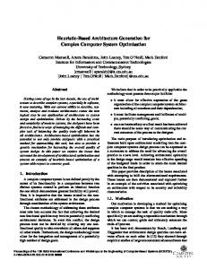
Fig. 2. Neural Field in a-solution. In this solution, when an input of a stimulus S(ϕ, t) is very large compared with the within-field cooperative interaction, a single-peak will be stabilized by interaction. It follows then the position of the stimulus maximum and remains there, even if the stimulus is removed.

by the convolution of an interaction kernel w(ϕ, ϕ). ´ That is, the activity change of a neuron ϕ depends on its actual activity level, the weighted input from other neurons, and the external input (stimulus) at its position. Depending on the parameter h, and the functions S, f , and w, equation (1) can have different types of solutions: 1. ∅-solution, if u(ϕ) ≤ 0, ∀ϕ. 2. ∞-solution, if u(ϕ) > 0, ∀ϕ. 3. a-solution, if there is localized excitation from a position a1 to a position a2 . This solution is also called a single-peak or mono-modal solution. In a-solution, weights in local neighborhood are stronger than those for large distances, which has the effect to stabilize a single peak at a position ϕ when a stimulus S(ϕ, t) is very large compared with the within-field cooperative interaction in that position. Furthermore, due to neurons interaction the peak remains in its position, even if we remove the stimulus. This interaction has also the effect to “push” the peak towards positions where the stimulus maximum is (Fig. 2). More detailed information can be found in [7][15]. III. N EURAL F IELDS

FOR

B EHAVIOR G ENERATION

The key idea of using neural fields in robotics navigation is to provide sensory information as stimulus to the neural field, and the position of the peak will decode the correspndant movement direction of the robot. In the experiments, the neural field has to encode angles from −π to +π divided into N discrete directions. Therefore, the model of (1) is first discretized as τ u(ϕ, ˙ t) = −u(ϕ, t) + S(ϕ, t) + h N X + w(ϕ, ϕ)f ´ (u(ϕ, ´ t)

(3)

ϕ=1 ´

We chose then its parameters such as an a-solution can be produced. The pre-activation of the field h = −1, the activation function f is chosen as a step-function  1, u ≥ 0 (4) f (u) = 0 u 0, and ϕT arget is the field position, equivalent to the main target direction at time t. B. Obstacle Stimulus This stimulus shows directions to obstacles {Sol (ϕ, t) : l ∈ [1, Nobst ]}, where Nobst is the number of obstacles detected by the robot sensors. It is chosen as gauss function centered at the direction of an obstacle. Sol (ϕ, t) = co e−σ(ϕ−ϕl )

2

(8)

where co is the amplitude of the obstacle stimulus. This parameter should be chosen stronger than target stimulus, since obstacle avoidance has a higer priority. The parameter σ defines the range of inhibition of an obstacle. In our case it was tuned regarding the radius of the robot and the influence of obstacles. ϕl reflects the direction of the obstacle l at time t. However, the stimulus considers only obstacles in distances dol which are below a threshold dT h . The contribution of all obstacles stimuli determine the final obstacle stimulus: Sobstacle (ϕ, t) =

N obst X

g(dol )Sol (ϕ, t)

(9)

l=1

where g is a step function:  1, dol < dT h g= 0 dol ≥ dT h

(10)

Using the step function g, only obstacles which their distances dol to the robot are below a threshold dT h are considered.

C. Global Stimulus The contributions of all stimuli determine the final state of the field, considering that obstacles stimulus must be taken inhibitory, since obstacles collision must be avoided. Thus, the global stimulus of the field at time t is determined by S(ϕ, t) = Starget (ϕ, t) − Sobstacle (ϕ, t)

(11)

D. Dynamics of Speed In a free obstacle situation, the robot moves with its maximum speed Vmax , and slows down when it approches a target. This velocity dynamics can be chosen as: VT (t) = Vmax (1 − e−σv dT )

(12)

where σv is a positive constant tuned in a relation with the acceleration capability of the robot. dT represents the distance between the robot and the target at time t. Close to obstacles, the robot needs also to be slowed down. In case of many obstacles, the nearest obstacle on the robot direction is considered. This dynamics can be chosen as: 2

VO (t) = CO (1 − g(dno )e−σOv (ϕF −inO ) )

(13)

where CO and σOv are positive constant, inO is the nearest obstacle direction to the robot movement direction and dnO is its distance relative to the robot. The final dynamics of the velocity is the contribution of (12) and (13). It is also considered when no appropriate direction can be selected, for example when the robot is completely surrounded by obstacles. In this case the robot must stop until the environmental situation changes. Thus, the robot velocity that satisfies the above design creteria is the following:  VT (t)VO (t), ϕF > 0 V (t) = (14) 0 ϕF ≤ 0 E. Passage between closely spaced obstacles The navigation system has been tested in the area of our institute using our indoor mobile robot STANISLAV, an RWI B21 robot (Fig. 1). It is 106 cm height and has a 52, 5cm diameter. It is equipped with 24 sonar sensors and a laser sensor for obstacle detection. Data measurment and control signals are managed through two internal computers, which are integrated via an on-board Ethernet. On the neural field we chose N = 60 neurons, which means that each direction N decodes a step of 6o . The neural field is expected to align the robot’s heading with the direction of the main target, and to bring it away from the nearby obstacles. The parameters m1 and m2 are chosen as 15 and 0, 45, respectively. Relative to those parameters we chose cO = 40 a stronger obstacle stimulus than the target, since obstacles have higher priority, and σ = 0.05 tuned according to the radius of the robot. This parameter is for safe movements near obstacles. With a closely spaced obstacles scenario we want to stimulate discussion on how good are DNFs comparing with the artificial potential fields (APFs) proposed by Khatib [16]. The basic idea of APF is to consider that the robot moves under influences of an artificial potential field. The target applies an

Fig. 3. Potential fields for target acquisition with avoidance of closely spaced obstacles. Note that the gap between obstacles A and C is only 90cm. When approching the gap (A-C), the robot moved under influence of repulsive forces exerted from obstacles A and C. This obliged it to turn away and it could not move through the gap.

attractive force to the robot, while obstacles exert repulsive forces onto the robot. The sum of all forces determines the subsequent direction of the movement. We implemented the APF method using a linear potential function on our robot and we obtained the results illustrated in Fig. 3. To highlight the adavantage of the neural fields approach, we tested the generation of behaviors: target acquisition and obstacle avoidance in the same scenario (Fig. 4). In the first 7 sec, both stimulus as well as field activation are unimodal, since no obstacles are detected and the stimulus contains only target entries. In the following time steps, the stimulus contains also obstacle entries. Therefore, it becomes bimodal. By contrast, on the field activation the peak moves to positions (decoding desired headings) corresponding to combination of target and obstacle stimuli. This allowed the robot to move through the gaps (A-C) and (B-C) until reaching the target point. Some photos from a video sequences of the performances of the two approaches are shown on Fig 5. However, it is important to mention that neural fields did not solve all problems from which APFs suffer. Experiments (not presented here) show that neural fields did not prevent the robot from being caught in a real local minima, i.e ”trapped” in dead-end situations, and the generated golbal paths are not necessarily the optimal ones. IV. C OMPLEX B EHAVIOR G ENERATION In this section we investigate how neural fields can be extended to generate more complex behaviors. The task at hand is inspired from biology. Eilman and Golani [17] show by experiments that when rats are brought in a novel environment, they move alternately between stop and go. The place in which they stay for the longest time is defined as the rat’s home-base. In addition, it was observed, that when they want to reach a target, they prefer going through these home-bases instead of going through novel routes. These home-bases are typically installed only in areas that are meaningful for them (e.g food places). We want to design a neural model such that it generates similar behaviors.

50

Activity

0

(a)

(b)

(c)

(d)

(e)

(f)

−50 25 −100 60

20 50

15 40 10

30 20

5

10 Neuron

0

Time

0

(a) neural field activation (peak position vs. time) Fig. 5. Photos from the video sequence of the closely spaced obstacles experiment. Neural Fields: (a) Approaching the gap. (b) Passing the first gap. (c) Passing the second gap and moving towards the target. Potential fields: (d) Approaching the gap. (e) and (f) repulsive forces obliged the robot to turn away. 40

Stimulus

20 0 −20 25 −40 60

20 50

15 40 10

30 20

5

10 Neuron

0

Time

0

(b) global stimulus 80 x y θ

60

40

20

0

−20

−40

−60 0

5

10

15

20

25

Time

(c) robot pose (x,y,θ) vs. time (sec)

However, it is not meant that we want to mimic a biological system like in [18][19]. Our aim is rather to show that it is possible to extend our neural field for generating more complex behaviors. In the navigation terminology, this can be seen as a case study in which a robot performs behaviors target-acquisition, obstacle-avoidance, and subtargetselection (predefined home-bases). A necessary condition is that the generated path should be the shortest one and through a maximum intermediate home-bases. Therefore, the neural field should produce a peak solution that satisfies two requirements: shortness and flexibility. By “shortness” we mean that a sub-target must be the nearest home-base to the robot and on the way to the main target. “Flexibility” is used here in the sense that the robot might change its destination to a new home-base in case of avoiding an obstacle. In this case the neural field needs extra information about homebases. A home-base becomes a sub-target if it fulfills the requirement of being the nearest one to the robot and on the way to the main target. Thus, an extra stimulus has to be designed, showing an attraction towards a sub-target. The choice between the main target and a home-base depends on the amplitudes of their stimuli. A higher amplitude of a stimulus means a higher priority will have the correspondant behavior. A. Home-base Stimulus We consider the quantity H contains all home-bases of the environment. The stimulus of each home-base h ∈ H is designed excitatory, showing an attraction towards a homebase as following Sh (ϕ, t) = h1 − h2 · ||ϕ, ϕh ||

(d) robot path Fig. 4. Neural fields for target acquisition with avoidance of closely spaced obstacles.

(15)

where h1 , h2 > 0, and ϕh is the field position, equivalent to direction of home-base h at time t. A home-base becomes a sub-target if it satisfies the requirements of being the nearest to the robot and to be located on the way to the main target. For this reason we multiply Sh with a gauss function 2 e−σT (ϕ−ϕT ) centred at the direction of the main target ϕT to

reduce the effect of all home-bases located outside a certain corridor leading to the target. In addition, we used another 2 gauss function e−σh (dh −r) to give more advantage to homebases lying closer to the robot. Here σh > 0 used to tune how big the advantage for nearest home-bases will be, dh the distance of a home-base h relative to the robot, and r is a radius arround a home-base in which the robot is considered to be at that home-base. The modified stimulus of a homebase h will be 2

2

Sh (ϕ, t) = e−σh (dh −r) e−σT (ϕ−ϕT ) (h1 − h2 · ||ϕ, ϕh ||) (16) where h = 1, 2, · · · Nh , and Nh the number of home-bases in the environment. The contribution of all home-bases stimuli defines the global sub-target stimulus. The contribution means that for each neuron we select the maximum value of stimuli at its position as follows Ssub−target (ϕ, t) = max{Sh (ϕ, t)| h ∈ H}

Fig. 6. Neural fields for target acquisition with sub-target selection. After turning on, the field receives entries from the target and home-bases 1 and 2. The effect of home-base 2 is reduced since it lies somewhat farther from the target than homebase 1. Moreover, adding up these stimuli gives more advantage for home-base 1 so that the maximum of stimulus will be on the corresponding neuron decoding its direction. After passing home-base 1, it can be seen that since no other home-bases are selected, the main target is acquired.

(17)

B. Global Stimulus The contribution of all stimuli including those of main target (eq. 7) and obstacles (eq. 9) determine the final state of the field input. Thus, the global stimulus of the field at time t is determined by S(ϕ, t) = Starget (ϕ, t) + Ssub−target (ϕ, t) −Sobstacle (ϕ, t)

(18)

Parameters of Ssub−target are chosen so that the summation with the main target stimulus will increase its amplitude. This gives an advantage to home-bases on the way to the target. A selection of a home-base means that its stimulus is higher than the main target, and consequently the neural field will generate a peak at that position. We will illustrate this concept through two scenarios. In the first scenario the field has to manage only two behaviors: target acquisition and sub-target selection without any obstacles (Fig. 6). This result demonstrates that the first requirement of shortening is fulfilled. The next experiment (Fig. 7) illustrates how the neural field manages three behaviors at the same time: target acquisition, sub-target selection, and obstacle avoidance. V. C ONCLUSION With this paper, we tried to show that it is possible to build a neural field model to perform three important and complex tasks for mobile robots: target aquisition, obstacle avoidance, and subtarget selection. First, we highlightted advantages of neural fields over potential field approach. The possibility to generate one single peak presents the power of this approach. This property could, for instance, solve some APF problems: oscillations in narrow passages and no passage between closely spaced obstacles [20]. In our earlier work [12] [13], this concept has shown also robustness against uncertainty in the perception system, and offered the robot the ability to adapt its behavior to unexpected

Fig. 7. Neural fields for target acquisition, obstacle avoidance, and subtarget selection. After starting, the field receives entries only from target and other home-bases. Through competition it selects home-base 2 as the next sub-target. After a while, the global stimulus contains also obstacle entries which has the effect to reduce the effect of the sub-target and to push the peak to another position. This means that the robot was obliged to avoid the obstacle. After avoiding the obstacle and passing the gap, home-bases 2 is not a potential sub-target any more. Instead, the home base 3 has the more advantage to be a sub-target, since in that new situation it lies better on the way to the target. After passing home-base 3, the main target is then acquired.

situations and navigate among static and moving obstacles. Moreover, the tuning of the field parameters is simple and does not depend on the environement. First, the field has to be forced to a-solution, in order to produce a single peak. Then, the stimulus is adjusted according to the task at hand. Further, we showed in this paper that the correct choice of stimuli parameters enables extension for more other behaviours, i.e. subtarget-acquisition. An important criterion is that the generated path should be the shortest path to the main target through the maximum intermediate home-bases. The global stimulus is designed in such a way that the nearest home-base has a stronger amplitude than the target. This has the effect to push the peak to the position decoding the direction of that home-base. Certainly, obstacles have always the strongest inhibitory amplitudes to maintain their highest priority. Based on this design the neural field could produce

solutions with respect to the requirements of shortness and flexibility. A future work will be the extension of the control design to another behaviour, namely moving in formation with other robots. In [14], we investigated how neural fields can offer a solution for the problem of moving multiple robots in formation, where the objective was to acquire a target, avoid obstacles, and keep a geometric configuration at the same time. We want to extend that framework by adding subtargets selection during the movement of a team of mobile robots. All in all, the experiments carried out here demonstrate the feasibility of the concept. However, despite these results, neural fields still need substantial inverstigation and more experiments to prove their generality in solving the problem of robot motion planning. R EFERENCES [1] Gregor Sch¨oner, Michael Dose, and Christoph Engels. Dynamics of behavior: Theory and applications for autonomous robot architectures. Robotics and Autonomous Systems, 16, 1995. [2] Axel Steinhage and Gregor Sch¨oner. Self-calibration based on invariant view recognition: Dynamic approach to navigation. Robotics and Autonomous Systems, 20:133–156, 1997. [3] Axel Steinhage and Gregor Sch¨oner. The dynamic approach to autonomous robot navigation. In ISIE97, IEEE International Symposium On Industrial Electronics, 1997. [4] T. Bergener, C. Bruckhoff, P. Dahm, H. Janßen, F. Joublin, R. Menzner, A. Steinhage, and W. von Seelen. Complex behavior by means of dynamical systems for an anthropomorphic robot. Neural Networks, 12(7-8):1087–1099, 1999. [5] S. Goldenstein, D. M. Metaxis, , and E. W Large. Nonlinear dynamic systems for autonomous agent navigation. In Proceedings of the Seventeenth National Conference on Artificial Intelligence. American Association for Artificial Intelligence., Menlo Park CA, 2000. [6] Sergio Monteiro and Estela Bicho. A dynamical systems approach to behavior-based formation control. In Proceedings of the 2002 IEEE International Conference on Robotics and Automation, Washington, DC, May 2002. [7] S. Amari. Dynamics of pattern formation in lateral-inhibition type neural fields. Biological Cybernetics, 27:77–87, 1977. [8] P. Dahm, C. Bruckhoff, , and F. Joublin. A neural field approach to robot motion control. In Proceedings of the 1998 IEEE International Conference On Systems, Man, and Cybernetics, pages 3460–3465, 1998. [9] M. A. Giese. Neural field model for the recognition of biological motion. In Second International ICSC Symposium on Neural Computation, Berlin, Germany, May 2000. [10] H. Edelbrunner, U. Handmann, C. Igel, I. Leefken, and W. von Seelen. Application and optimization of neural field dynamics for driver assistance. In IEEE 4th International Conference on Intelligent Transportation Systems, pages 309–314. IEEE Press, 2001. [11] Wolfram Erlhagen and Estela Bicho. The dynamic neural field approach to cognitive robotics. Journal of Neural Engineering, 3:R36– R54, 2006. [12] M. Oubbati, M. Schanz, and P. Levi. Neural fields for behaviourbased control of mobile robots. In 8th International IFAC Symposium on Robot Control. Bologna, Italy., September 2006. [13] M. Oubbati and G. Palm. Neural fields for real-time navigation of an omnidirectional robot. In European Conference on Mobile Robots, Freiburg, Germany., 19–21 September 2007. [14] M. Oubbati and G¨unther Palm. Neural fields for controlling formation of multiple robots. In IEEE International Symposium on Computational Intelligence in Robotics and Automation (CIRA2007), Jacksonville, Florida, USA, pages 90–94. IEEE, 20-23 June 2007. [15] Kishimoto K. and Amari S. Existence and stability of local excitations in homogeneous neural fields. Journal of Mathematical Biology, 7:303–318, 1979.

[16] O. Khatib. Real-time obstacle avoidance for manipulators and mobile robots. International Journal of Robotic Research, 5(1):90–98, 1986. [17] D. Eilam and I. Golani. Home base behavior of rats (rattus norvegicus) exploring a novel environment. Behavioural Brain research, 34:199– 211, 1989. [18] Mataric Maja J. Navigating with a rat brain: a neurobiologicallyinspired model for robot spatial representation. In First International Conference on Simulation of Adaptive Behavior, pages 169–175, Cambridge,MA, 1990. MIT Press. [19] Matthias O. Franz and Hanspeter A. Mallot. Biomimetic robot navigation. Robotics and Autonomous Systems, 30:133–153, 2000. [20] Y. Koren and J. Borenstein. Potential field methods and their inherent limitations for mobile robot navigation. In Proceedings of the IEEE Conference on Robotics and Automation, pages 1398–1404, April 1991.