for non-linear time series, M. Mangeas and J.F. Yao [6] proposed an identification criterion of neural architectures. So, for a given series of. T observations, we ...
Neural Model Selection: How to Determine the Fittest Criterion? M o r g a n MANGEAS
Universitd Paris 1, research center SAMOS 90 rue de Tolbiac,75634 Paris Cedex 13, France
Electricitd de France, Research Center 1, avenue du g~n~ral de Gaulle 92141 Clamart cedex, France
A b s t r a c t . Based on recent results about the least-squares estimation for non-linear time series, M. Mangeas and J.F. Yao [6] proposed an identification criterion of neural architectures. So, for a given series of T observations, we know that for any 7 E T~+* the selected neural model (architecture + weigilts) that minimize the least square criterion LSC -- MSE + 71nT/T × n (the term n denotes the number of weights) converges almost surely towards the "true" model, when T grows to infinity. Nevertheless, when few observations are available, an identification method based on this criterion (such the pruning method named Statistical Stepwise Method (SSM) [1]) can yield different neural models. In this paper, we propose a heuristic for setting the value of ~/up, with respect of the series we deal with (its complexity and the fixed number T). The basic idea is to split the set of observations into two subsets, following the well-known cross-validation method, and to perform the SSM methodology (using the the LSC criterion) on the first subset (the learning set) for different values of 7. Once the best value of ~ is found (the one minimizing the MSE on the second subset (the validation set)), we can use the identification scheme on the whole set of data.
1
Introduction
In a statistical framework, to avoid overfitting means to resolve the p r o b l e m of identification I a n d estimation 2. In this paper we describe a heuristic t h a t a t t e m p t s t o resolve this problem in the field of forecasting time series. Since we want perform a u t o m a t i c model selection, we choose to select models in the largest class of feedforward neural networks. This class is c o m p o s e d of networks w i t h o u t layer structure (see an example on figure 1) and includes the multilayer perceptron class. Let us consider a general feedforward network c o m p o s e d of rn input units, n hidden units and an o u t p u t unit. To avoid feedback connection, we label the hidden units by ( h i , h 2 , . . . , hn}, and we decide an a r b i t r a r y order relation: hi can connect to hi, only if i < j . As usual, the input units receive no connection, 1 To find the suited model structure (the architecture). 2 To estimate the suited set of parameters (synaptic weights).
988
but can connect to each hidden unit and to the output unit, and the output unit can be connected to any other units. The units sum the values provided by the previous units, weighted by the synaptic coefficients, and apply a trans]er function. Since we perform regression, we conventionally associate linear transfer function to the input and output units 3, and a sigmoid transfer function to the hidden units. input unit
mit
Fig. 1. Example of feedforward neural network. This one has 7 input units (denoted a,b,...,g), 3 hidden units (denoted 1,2,3) and one output unit (denoted o).
Let f w be the function that denotes the neural model. We denote A its architecture and W the vector of weights. The term I?VA,T denotes the estimator of W for the fixed architecture A for a number fixed T of observations:
I?VA,T = argm~n with
ST(A)
(1)
T
ST(A) = ET=v+I(Xt - fw(Xt-1, Xt-2,..., Xt-p, Yt, 1)) 2
Thus, by applying the existing results [3] and [2], on model selection by penalized contrasts, M. Cottrell, J.F. Yao and M. Mangeas [6, 5] establish an almost sure identification of a true model, when there are a finite number of possible models having a common dominant architecture. This method has been extensively analysed and compared to other model selection methods such OBD [4].
2
Almost
sure
identification
of a true
model
More precisely, assume that we have a fixed bound M for all possible model dimensions. Thus let W be the space where the weights are living (W 6 )4; C 3 The output unit can be straightly connected to the input unit. So, this model can include a linear combination of the inputs (MLPs can not).
989 7¢M) and Amax be a dominant architecture, whose parameter vector is denoted Wmax = (Wl, W2,... ,WM). Consider the finite family `4 = {(wl, w 2 , . . . , WM)/ some components are set to 0}, respecting a set of constraints linked to the interpretation of the components of W in the neural network. For a A E ,4, sub-architecture of Amax, we denote by n(A) the number of its non null weights, i.e. the dimension of the parameter vector W, and ~)A the set of possibles values of W. The true model, which is a sub-model of Amax, is denoted by A0 and the true value of the parameter vector is W0 with dimension m(Ao). Let (c(t)) be a positive sequence of real numbers. The penalized least-squares contrast with penalization rate (c(t)) takes the form LSC(T, A) - -ST(A) -T-- +
n(A).
(2)
Let f~T = ArgminAe.4LSC(T,A) be the estimated architecture, which is the result of two successive minimizations for a fixed T: - a minimization on a continuous space, to compute I$~T,A, ST(A), a minimization on a finite space, to compute AT. -
With these definitions, the following result and its complete proof can be found in [6].
Assume that the conditions a about the asymptotic normality of the weights hold [6]. Suppose also the penalization rate c(T) is such that
Theorem 1
lim
c(T)
T T
"~ O,
and
c(T)
limTinf ~ Inin 2 T >
o2 A
--)~
(3)
where A (resp. ~) is the largest (resp. smallest) eigenvalue o] the matrix Zo. Then, the pair (AT, ITVT,AT ) converges a.s. to the true value (A0, Wo). We can now propose an almost sure identification methodology to determine the true model within the set of the Amax sub-models: Let the term V be some positive constant. A logarithmic penalization rate c(t) = 7 In t clearly meets the above conditions (3). Taking such a penalization rate yields the following least squares criterion (LSC) for model selection: LSC = LSC(T, A) - ST(A) T + 7 ~ _ n(A)
(4)
Theoretically, in order to estimate the true model, we would have to exhaustively explore a finite family and compute the LSCs for all sub-models A E .4. But the number of these sub-models is exponentially large (as 2 M) and it is impossible to do it in practice. So, as in linear regression analysis, we propose a Statistical Stepwise Method (SSM) to guide the search in .4. See [1] for previous presentations of the SSM algorithm, with several examples. Using the results 4 These weak conditions concern a control over the noise, over the weights space, and over the identifiability of the model.
990
about the almost sure identification model, we have a theoritical stopping criterion: the LSC. The principle is to stop the deletion as soon as the criterion LSC increases. Nevertheless, if the value of 7 can be, in theory, any positive real when T is very large, this assertion becomes not true when few observations are available. So, an identification method based on this criterion (such the pruning method SSM can yield different neural models. At this stage, it seems interesting to propose a heuristic for setting the value of V up, with respect of the series we deal with (its complexity and the fixed number T). To resolve this problem, we propose to use the well-known cross-validation approach in order to compute the suited value of 7. The basic idea is to split the set of observations into two subsets. The SSM algorithm is performed on the first subset (the learning set) for different values of 7- On the second subset (the validation set) we can determine the value of 7 that gives the best performance (the one that minimizes the MSE). Once the best value of 3, is determined, we can use the SSM identification scheme on the whole set of data, without loss of information, and with a suited stopping criterion. It is worthy to note, that this methodology is correct only if the series is stationnary. So, as for the famous early stopping method, the validation set should be extract with caution, in order to avoid some significant statistical differences between the distributions of the sets of data. 3
Applications
In order to investigate the feasibility of this method, we apply the heuristic to two time series. The first series is the widely studied sunspots series. The second one is a standard series from the french power company: the daily electricity demand. Each series is modelled following the same scheme: 1. to randomly extract two subsets from the whole set of data associated to the series (included exogenous variables), 60% for the learning set, 40% for the validation set, 2. to choose a dominant architecture, 3. to apply the SSM method on the learning set using different values of 7, 4. to determine the suited value of 7 (the one minimizing the MSE on the validation set), 5. to apply the SSM method on the whole set of data, using the previously determined value of 7. For the sunspots series, we start (step 2) with a dominant neural architecture with 80 synaptic weights. In order to determine the suited value of 7 (step 4), we perform 11 runs of SSM with 7 E {0,0.01,0.02,...,0.1). You can see on figure 2, the curves of the performance of the selected models (after applying the SSM method) on the learning set and on the validation set, in function of the value of 7- Following the cross-validation approach (step 4), the best value is bounded by 0.036 and 0.064. For these values, around 32 weights are pruned. After rerunning the SSM method on the whole set of data (step 5), we remark
991
~g
0.0
0.04 g a m m a
0.08
Fig. 2. Forecasting the sunspots series. The plain line characterizes the MSE of the final model (after applying the SSM algorithm with a certain value of 7) computed on the learning set. The dotted line characterizes the MSE computed on the validation set, and the dashed line characterizes the number of weights.
that 31 weights are pruned and the final value of the MSE is equal to 0.06. This value is contained between the values of the MSE of the previous best estimated model on the learning set and on the validation set. The SSM method needs in average 5 minutes of CPU time. So the whole process of model selection is completed in about one hour of CPU time on a sparc station 20. Forecasting electricity demand (i.e. power loads) is a crucial problem for Electricit6 de France (EDF) (see [7]). For this series we start (step 2) with a dominant neural architecture with 400 synaptic weights. In order to determine the suited value of 7 (step 4), we perform 11 runs of SSM with 7 E {0,0.02,0.04,...,0.2}. You can see on figure 3, the curves of the performance of the selected models (after applying the SSM method) on the learning set and on the validation set, in function of the value of 7. Following the cross-validation approach (step 4), the best value is bounded by 0.03 and 0.04. For these values, around 35 weights are pruned. After rerunning the SSM method on the whole set of data (step 5), we remark that 38 weights are pruned and the final value of the MSE is equal to 0.0297. This value is contained between the values of the MSE of the previous best estimated model on the learning set and on the validation set. The SSM method needs in average 10 minutes of CPU time for this example. So the whole process of model selection is completed in about two hours of CPU time on a sparc station 20. In comparison with some other neural model, this final model is performant as well as robust with regard of the generalization ability.
4
Conclusion
In this paper, we have shown the feasibility of the method that consists in setting a model selection criterion up with respect of the complexity of the problem and the number of available observations. The associated model selection method
992
\
\
\
J~z
\
E0.0
0.08 gamma
0.16
Fig. 3. Forecasting the daily electricity demand, see figure 2 for explanations about the curves. (using this criterion and the pruning method SSM) is easy to implement, yield suited model and consume reasonable CPU time. This heuristic comes from a theoritical frame, but the use of a validation set makes this method fragile. In particular, one have to assume that the series is stationnary. If the validation set has different statistical properties than the learning set, this assumption can be wrong. If not, the computed value of 7 can be used to determine the suited model on the whole set of data, without loss of information. We validate this identification method of feedforward neural model on two different real-world series. The results show the consistency of the performance of the selected neural models, and encourage to apply this identification method to other forecasting problems.
References 1. M. Cottrell, B. Girard, Y. Girard, M. Mangeas, and C. Muller. Neural modeling for time series : a statistical stepwise method for weight elimination. LE.E.E. Trans. Neural Networks, 6:1355-1364, 1995. 2. M. Duflo. Algorithmes Stochastiques. Math~matiques & Applications (SMAI). Springer-Verlag, Berlin(1996. 3. X. Guyon. Random Fields on a Network - Modeling, Statistics, and Applications. Springer-Verlag, Berlin, I995. 4. Y. le Cun, J. S. Denker, and S. A. Solla. Optimal brain damage. In D. S. Touretzky, editor, Advances in Neural Information Processing Systems 2 (NIPS*89), pages 598605, San Mateo, CA, 1990. Morgan Kaufmann. 5. M. Mangeas, M. Cottrell, and J.F. Yao. New criterion of ideatification in the multilayered perceptron modelling. In Proceedings of ESANN'97, Bruges, Belgium, 1997. 6. M. Mangeas and Jian-feng Yao. Sur l'estimateur des moindres carr~s d'un module autor~gressif non-lin~aire. Technical Report 53, SAMOS, Universit~ Paris I, 1996. 7. A. S. Weigend and M. Mangeas. Avoiding overfitting by locally matching the noise level of the data. In World Congress on Neural Networks (WCNN'95), pages II-1-9, 1995.