for Aerospace. Information. 800 Elkridge. Landing Road. Linthicum. Heights,. MD 21090-2934. Price Code: A03. Available from. National Technical Information.
NASA/TMB1998-206316
Neural
Network
and Regression
Approximations Transport
Surya N. Patnaik Ohio Aerospace
in High
Aircraft
Institute,
Cleveland,
James
D. Guptill,
Dale A. Hopkins,
Lewis
Research
Center,
National
Aeronautics
Space
Administration
Lewis
Research
April
1998
Center
Design
Cleveland,
and
Speed
Optimization
Ohio
and Thomas Ohio
Civil
M. Lavelle
Trade names or manufacturers' names are used in this report for identification onl3a This usage does not constitute an official endorsement, either expressed or implied, by the National Aeronautics and Space Administration.
Available NASA Center for Aerospace Information 800 Elkridge Landing Road Linthicum Heights, MD 21090-2934 Price Code: A03
from National
Technical
Information
Service
5287 Port Royal Road Springfield, VA 22100 Price Code: A03
NEURAL NETWORK AND REGRESSION SPEED CIVIL TRANSPORT AIRCRAFT
APPROXIMATIONS IN HIGH DESIGN OPTIMIZATION
Surya N. Patnaik* Ohio Aerospace Institute, Brook
Park, Ohio
James D. Guptill t, Dale A. Hopkins', and Thomas M. Lavelle§ National Aeronautics and Space Adminstation Lewis Research Center Cleveland,
Ohio 44135
SUMMARY Nonlinear mathematical-programming-based design optimization can be an elegant method. However, the calculations required to generate the merit function, constraints, and their gradients, which are frequently required, can make the process computationally intensive. The computational burden can be greatly reduced by using approximating analyzers derived from an original analyzer utilizing neural networks and linear regression methods. The experience gained from using both of these approximation methods in the design optimization of a high speed civil transport aircraft is the subject of this paper. The Langley Research Center's Flight Optimization System was selected for the aircraft analysis. This software was exercised to generate a set of training data with which a neural network and a regression method were trained, thereby producing the two approximating analyzers. The derived analyzers were coupled to the Lewis Research Center's CometBoards test bed to provide the optimization capability. With the combined software, both approximation methods were examined for use in aircraft design optimization, and both performed satisfactorily. The CPU time for solution of the problem, which had been measured in hours, was reduced to minutes with the neural network approximation and to seconds with the regression method. Instability encountered in the aircraft analysis software at certain design points was also eliminated. On the other hand, there were costs and difficulties associated with training the approximating analyzers. The CPU time required to generate the input-output pairs and to train the approximating analyzers was seven times that required for solution of the problem.
INTRODUCTION Intensive computation can be a serious deficiency in an otherwise elegant nonlinear mathematicalprogramming-based design optimization method. In typical structural design applications, most of the computations, often more than 99 percent of the total calculations, can be traced to the analyzer (ref. 1). That is, reanalysis and sensitivity calculations consume the bulk of the computation time in design optimization. To reduce the computational burden, two approximation methods, regression analysis and neural networks, have been incorporated into the NASA Lewis Research Center's design test bed CometBoards (refs. 1 to 3) (Comparative Evaluation Test Bed of Optimization and Analysis Routines for the Design of Structures). Both approximation methods provide the reanalysis and design sensitivity information that is usually required during optimization. Approximation augmentation, which includes a strategy to select training pairs, has broadened the scope of CometBoards; thus, a design problem can be solved by using three different analyzers the original analyzer or one of the two derived analyzers that are based on regression and neural networks. The example of a high speed civil transport (HSCT) aircraft is considered to examine the performance of approximation methods in design optimization. The NASA Langley Research Center's Flight Optimization System, FLOPS (refs. 4 and 5), which is well known in industry, was chosen as the aircraft analyzer. This analyzer is not just
*Engineer,
Associate
tMathematician, _;Acting Chief, §Engineer,
Fellow
Structural
Propulsion
No copyright
NASA/TM--
AIAA.
Computational
is asserted
Sciences
Mechanics System
Analysis
in the United
1998-206316
Branch.
Branch,
Senior
Member
AIAA.
Office. States.
1
computationally intensive;
it can also become unstable at certain design points, thereby requiring that the optimization process be restarted. Moreover, an optimum benchmark solution established for the HSCT aircraft problem from results generated previously with the FLOPS analyzer by Langley, Lewis, and industry becomes a useful solution against which the results obtained with the approximation methods can be compared. CometBoards, which includes an approximation module containing regression analysis as well as neural networks, has been soft-coupled to the FLOPS analyzer. The CometBoards-FLOPS combined software can optimize an HSCT aircraft by using any one of the three analyzers--the original FLOPS code, the derived regression, or neural network models. This paper presents optimal solutions that were generated for the HSCT aircraft by using all three analyzers. The results are examined to assess the performance of the approximation methods in the design of an HSCT aircraft system. In specific terms, the deviation in the aircraft weight and behavior constraints, and their sensitivity, are investigated for analysis as well as design. The computational efficiency achieved by using approximation methods in design optimization is examined by comparing CPU solution times. This paper is organized as follows: an overview of the CometBoards design test bed; a brief description of the aircraft analyzer FLOPS; a strategy to generate the input portion of the input-output (io) pairs for training both approximating analyzers; a brief description of regression analysis and neural networks; a definition of the design problem and the benchmark solution; generation of the io pairs for this problem; representative response prediction through the approximation methods; the performance of both approximation methods in predicting the behavior parameters of the aircraft; their performance during design optimization; and conclusions.
COMETBOARDS:
A DESIGN
TEST BED
Our earlier research to compare different optimization algorithms and alternate analysis methods for structural design applications has grown into a multidisciplinary design test bed that is still referred to by its original acronym, CometBoards. The modular organization of CometBoards (see fig. 1) allows innovative methods to be quickly validated through the integration of new programs into its existing modules. Optimizers and analyzers are two important modules of CometBoards. The optimizer module includes a number of algorithms, such as the fully utilized design (ref. 6), optimality criteria methods (ref. 6), the method of feasible directions (ref. 7), the modified method of feasible directions (ref. 8), three different sequential quadratic programming techniques (refs. 9 to 11), the Sequential Unconstrained Minimizations Technique (ref. 12), sequential linear programming (ref. 7), a reduced gradient method (ref. 13), and others. Likewise, the analyzer module includes COSMIC/NASTRAN (ref. 14), the nonlinear analyzer MHOST (ref. 15), the U.S. Air Force ANALYZE/DANALYZE (ref. 16), IFM/ANALYZERS (ref. 17), the aircraft flight optimization analysis code FLOPS (ref. 5), the NASA Engine Performance Program NEPP (ref. 18), and others. Some of the other unique features of CometBoards include a cascade optimization strategy, design variable and constraint formulations, a global scaling strategy, analysis and sensitivity approximations through regression and neural networks, and substructure optimization on sequential as well as parallel computational platforms (ref. 19). CometBoards has provisions to accommodate up to l0 different disciplines, each of which can have a maximum of 5 subproblems. The test bed can optimize a large system, which can be defined in as many as 50 different subproblems. Alternatively, a component of a large system can be optimized in order to improve an existing system. The design test bed has been successfully used to solve a number of problems, such as the structural design of space station components; the design of nozzle components for air-breathing engines; and the configuration design of subsonic and supersonic aircraft, mixed flow turbofan engines, and wave rotor concepts in engines. CometBoards has over 50 numerical examples in its test bed. It is written in FORTRAN 77, except for the neural network code, Cometnet (ref. 20), which is written in C++. The process of integrating this C++ code into the CometBoards FORTRAN 77 code is referred to as soft-coupling. Soft-coupling is achieved by first generating an executable file from the Cometnet C++ source code; then Cometnet is invoked from CometBoards through a system call. Information is exchanged between the two programs through data files. At present CometBoards is available on UNIX-based Cray and Convex computers and on Iris and Sun workstations. CometBoards is continuously being improved to increase its reliability and robustness for optimization at system as well as component levels. This paper emphasizes the approximation module of CometBoards, which includes regression analysis and neural network approximations for the design optimization of an HSCT aircraft.
NASA/TM--1998-206316
2
FLOPS: ANAIRCRAFT ANALYZER Aircraftdesign wasformulated asanonlinear programming problem withasetofdesign variables tooptimize ameritfunction underasetofbehavior constraints. TheFLOPS analyzer evaluated theperformance parameters of anadvanced aircrafttogenerate theconstraints andmeritfunction. Bysoft-coupling Lewis'CometBoards and Langley's FLOPS, thedesign problem couldbesetupandsolved withoutmajormodification toeithercode.The design problem wassolved byusingtheCometBoards-FLOPS combined capability. TheFLOPS analyzer haseightdisciplines: weightestimation, aerodynamic analysis (refs.21and22),engine cycleanalysis (refs.23to25),propulsion datainterpolation, mission performance, airfieldlengthrequirements for takeoffandlanding, noisefootprint calculations (ref.26),andcostestimation (refs.27to32).TheFLOPS analyzer allowsselection ofthefollowingfreevariables forthepurpose ofoptimization: (1)rampweight, (2)wingaspect ratio,(3)engine thrust,(4)taperratioofthewing,(5)reference wingarea,(6)quarter chordsweep angleofthe wing,(7)wingthickness tochordratio,(8)cruise Machnumber, (9)cruisealtitude, (10)engine design pointturbine entrytemperature, (11)overall pressure ratio,(12)bypass ratioforturbofan engines, (13)fanpressure ratiofor turbofan engines, and(14)engine throttleratio(defined astheratioofmaximum allowable turbineinlettemperature dividedbythedesign pointturbineinlettemperature). FortheHSCTproblem, thefreevariables wereseparated into asetofsixactivedesign variables andasetofeightpassive design variables. Forthepurpose ofoptimization, thecomposite meritfunction available inFLOPS canbewrittenas 7 (1)
Obj = ___ Wk#k k=l where Obj represents the merit function, wk represents the kth weight factor, and the parameter flk can be selected from the following list: (1) gross takeoff weight of the aircraft, (2) mission fuel, (3) the product of the Mach number times the ratio of lift-to-drag, (4) range, (5) cost, (6) specific fuel consumption, and (7) NOx emissions. For the HSCT problem, the gross takeoff weight was selected as the merit function by setting w I =1.0 and the other weight factors to zero. Behavior constraints can be imposed on (1) the missed approach climb gradient thrust, (2) the second-segment climb thrust, (3) the landing approach velocity, (4) the takeoff field length, (5) the jet velocity, (6) the compressor discharge temperature, (7) the total usable fuel weight, (8) the range of the flight, (9) the landing field length, (10) the aspect ratio (defined as the ratio of bypass area to the core area of a mixed flow turbofan engine), (11) the engine-throttle ratio, (12) the specific fuel consumption, (13) the compressor discharge pressure, (14) the excess fuel, and others. Only the first six constraints were imposed in the HSCT problem. The design space of an aircraft optimization problem can be distorted because both design variables and constraints vary over a wide range. For example, an engine thrust design variable (which is measured in kilopounds, e.g., 40 000 lb) is immensely different from the bypass ratio variable (which is a small number, e.g., 0.5). Likewise, a landing velocity constraint in knots and a field length limitation in thousands of feet differ both in magnitude and in units of measure. In CometBoards the distortion is reduced by scaling the merit function, design variables, and constraints such that their normalized values are around unity.
SELECTION
STRATEGY
FOR INPUT
PORTION
OF INPUT-OUTPUT
PAIRS
FOR TRAINING
Both regression and neural network approximations require a set of io pairs for their training. Since intrinsic coupling of design variables can be inherent to large design problems, this coupling can be exploited to increase the efficiency of the training scheme. A strategy has been devised to generate a set of design variables that forms the input portion of the training pairs for a specified coupling map. The output portion, representing the merit function and behavior constraints, is generated from the FLOPS analyzer for the specified input design variables. An example of a design problem with six active variables (1 to 5 and 7) and one passive variable (6) is used to illustrate the input variable selection strategy. The six active variables are separated into four related sets, designated by circled digits 1 to 4 in figure 2. The design variables are shown in braces: {4,7}, {2}, {3,5}, and { 1,2,7} for sets 1 through 4, respectively. Their coupling and influence regions, shown in figure. 2, are given in table I.
NASA/TM--1998-206316
3
In table I consider, for example, Set 3 with two influence regions (2 and 4, see fig. 2). Response prediction for Set 3 (with two active design variables of its own) will include those of its coupling regions (design variables 1, 2, 3, 5, and 7). These five variables will be perturbed by using the scheme described next, and in addition, other active variables may also undergo minor perturbations. Consider a design variable in a set with initial design Zi, upper bound Z u, and lower bound XI. Divide the interval between the lower bound and the initial design, and that between the initial design and the upper bound, into nil and niu subintervals, respectively. A bandwidth bw is assigned for the design variable that specifies the number of subintervals to be grouped together to form random perturbations. To illustrate the strategy for selecting the input portion of a set of io pairs, let us consider a simple example with two design variables. The perturbation scheme requires the following data for each design variable: (1) Design (2) Design
variable 1: lower, initial, and upper bounds of, for example, variable 2: lower, initial, and upper bounds of, for example,
0.05, 4.00, and 10.00, respectively. 0.50, 6.00, and 9.50, respectively.
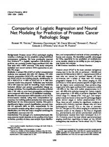
Let us divide the intervals between the lower bound and the initial design into four subintervals. Likewise, divide the interval between the initial design and the upper bound into three subintervals. Assume a bandwidth of bw = 3. Further, specify the number of perturbations for each subinterval as follows: for the four subintervals beginning from the initial design toward the lower bound--15, 10, 2, and 6; and for the three subintervals from the initial design to the upper bound--10, 4, and 8. The input portion of the io pairs generated through the selection strategy is depicted in figure 3. There are 131 design points. The inner circle, with a radius of 2 centered on the initial design (4,6), captures 31 design points, which corresponds to a density of 2.5 points per unit area. The annulus with radii of 2 and 3 also contains 31 design points, but is less dense with 2.0 points per unit area. A satisfactory pattern for the input portion of the io pairs can be generated by changing the bandwidth, number of intervals, stations, and perturbations in an iterative fashion.
Linear Regression
Analysis
Regression analysis available in CometBoards uses several basis functions. The basis functions can be selected from (1) a full cubic polynomial, (2) a quadratic polynomial, (3) a linear polynomial in reciprocal variables, (4) a quadratic polynomial in reciprocal variables, and (5) combinations thereof. Consider, for example, regression analysis of an n variable model with a combination of a cubic polynomial in design variables and a quadratic polynomial in reciprocal design variables. The regression function has the following explicit form: n
y(_)=
flO + 2flixi i=1
The regression
coefficients
n
/I
+EEflijxixj i=1
j=i
]_ are determined
n
/1
+2E i=1
n
2flijkXiXjXk
/,1
+ 2_i
j=ik=j
i=1
by using the linear least squares
/I
n
l_._+E Eflij_
approach
i=1
xixjl
(2)
j=i
incorporated
in the DGELS
(double precision general matrix linear least squares solver) routine of the Lapack library (ref. 33). The gradient matrix of the regression function with respect to the design variables is obtained in closed form. For the example with n variables, the gradient matrix for the regression function has the following form: "0 O_Xl
0 Vy =.0x
2 y
OnXn where
NASA/TM--
1998-206316
4
(3)
OqXl
i=l
i=l
j=i+l
i=1
j=i
"=
and fl(i = _jifori>j, _i)k= flikj forj> k > i,etc. Once theregression coefficients have been obtainedfrom thesingletraining cycle,reanalysis and sensitivity calculations represented by equations(2)to (4)requiretrivial computationaleffort. In regression analysis, the accuracy oftheapproximationfunctionand itsgradientcan differsignificantly near,as wellas outsideof,theboundary of thetraining domain. Thisdeficiency, ifany,inCometBoards can be reducedby selecting eitherclosed-formor finite difference gradients, atthe discretion of theuser.
NEURAL
NETWORK
APPROXIMATIONS
The neural network approximator available in CometBoards, Cometnet, is a general-purpose object-oriented library. Cometnet is soft-coupled to the CometBoards test bed. The neural network capability provides both function values and their gradients. Cometnet approximates the function and its gradient with R kernel functions as follows:
g
tl r
Y( x ) : _._ E r=l
i=l
R
nr
(Sa)
Wri_Ori('r)
C_(Pri(.________ )
dY( )-EEw" dx, OqX_
where y is the functional
approximation,
(5b)
r=l i=1
._ is the vector of independent
variables, tpr/ represent
R kernel functions,
n r represents the number of basis functions in a given kernel, and Wr/are the weight factors. Cometnet permits approximations by using different kernels, which include linear, reciprocal, and polynomial, as well as Cauchy and Gaussian radial functions. A Singular Value Decomposition algorithm (ref. 34) for computing the weight factors in the approximating function is used to train the network. A clustering algorithm is used to select suitable parameters for defining the radial functions. The clustering algorithm, in conjunction with an optimizer, seeks optimal values for the parameters over a range for the threshold parameter "rwithin its domain (0 < z < 1). The mean-square error during training is reduced by increasing the threshold, which corresponds to an increase in the number of basis functions. Over-fitting is avoided with a competing complexity based regularization algorithm, which is given in reference 35. The merit function, and each of the constraint functions can be trained separately by using different basis functions.
DEFINITION
OF THE HSCT AIRCRAFT
DESIGN
PROBLEM
The HSCT aircraft problem devised by NASA Langley Research Center was employed to examine the performance of the approximation methods for both analysis and optimization (ref. 24). This supersonic aircraft was to be powered by four mixed-flow turbofan engines. The mission requirement of the aircraft was to carry 305 passengers at a cruise speed of Mach 2.4 for a range of 5000 n mi. The objective of the optimization was to determine the airframe-engine design combination that would meet these constraints with a minimum gross takeoff weight. A good match between the engine and airframe can be achieved by combining the engine parameters with the airframe variables. Six active design variables were selected to optimize the design. There were two airframe design
NASA/TM--1998-206316
5
variables--the engine thrustandthewingsize--and fourengine design parameters---the turbineinlettemperature, theoverallpressure ratio,thebypass ratio,andthefanpressure ratio.Theturbineinlettemperature waslimitedtoa maximum of3560°R. The constraints imposed on the aircraft and engine were as follows: The takeoff and landing field lengths had to be less than 11 000 ft; the approach velocity had to be less than 160 kn; there had to be enough volume to carry all the required fuel; there had to be enough engine thrust available to recover from a missed approach and execute a second-segment climb; the exit jet velocity had to be less than 2300 ft/sec to limit engine noise; and the compressor discharge temperature had to be less than 1710 °R. To assess the performance of the approximation methods, the design space was divided into three subregions: the standard, wide, and restricted ranges. The range used to train the approximating analyzers is referred to as the standard range and designated with the letter "b" in table II. The wide range, designated by the letter "a," is defined as the range outside the training range. The restricted range, designated by the letter "c," is defined as the range inside the training range. The design variables, their ranges, and status (active or passive) are specified in table II. The six behavior (1) Missed
constraints,
approach
which are implicit
functions
of the design
climb thrust tc, which must be positive;
variables,
were as follows:
it was normalized
with respect
to 106 Ib
it was normalized
with respect
to 104 lb
tc