National Computer Science and Engineering Conference (NCSEC 2006) 25-27 October 2006 P83
Neural Network Based Greedy Job Scheduler Kothalil Gopalakrishnan Anilkumar and Thitipong Tanprasert Department of Computer Science, Faculty of Science and Technology, Assumption University, Soi 24, Ram Khamhaeng Road, Hua Mak, Bang Kapi, Bangkok 10240, Thailand.
[email protected],
[email protected]
scheduling allows the representation by fuzzy sets and linguistic variables and the inference from vaguely formulated knowledge [5].The main disadvantage of this approach is that, it needs tremendous computational effort to handle complex industrial problems. In this paper we propose a 3-layer feed-forward backpropagation NN to assign priority for each queued job which is humanly subjective in nature. Train the NN to get priorities by using backpropagation algorithm [6], which is the most famous supervised training algorithm. Furthermore, a ‘greedy method’ is used to build up possible feasible schedules by improving the objective function during each stage of the scheduling process. The organization of this paper is as follows: Section two describes structure of the scheduler, section three presents in detail, the NN as priority assigner, section four describes the greedy alignment procedure with backpropagation algorithm, section five presents simulation of the scheduler with various jobs and machine sizes and finally, section six concludes this paper.
Abstract This paper presents a greedy job scheduler using a 3-layer feed-forward Neural Network (NN) and a greedy alignment procedure. The NN is used to assign priority of queued jobs which is humanly subjective in nature. Output of the NN is used by the greedy alignment procedure to schedule each job on respective machine with feasible Finishing Time (FT). Machines used in this paper are non identical in nature and are ordered based on their capacity before they start to process each job. Optimality of the given schedule is estimated based on the average duration of n jobs over m machines. Simulations are made to analyze the performance of the proposed scheduler with various jobs and machine sizes. Simulation results show that the proposed scheduler is the best one for feasible schedules. Key Words: Backpropagation, duration, deadline, critical type, priority, greedy alignment procedure, finishing time.
1. Introduction
2. Description of the scheduler
Scheduling refers to the act of assigning resources to tasks or assigning tasks to resources. Traditionally there are three kinds of approaches for the solution of job scheduling problems: priority rules, combinatorial optimization, and constraint analysis [1]. Hopfield first used a neural network [2] to solve optimization problems. Neural networks are parallel, tolerant to noise, and self-organizing, and they also approximate functional relationships between cause and effect [3]. Many approaches have been used to find solution to job scheduling problems. Dispatch rules are used to solve job scheduling problems [4]. These rules lack a global view of the shop and they usually build up a large amount of bottleneck in a complex industrial situation. Fuzzy based
This section describes various parameters used by the scheduler such as; a set of independent jobs {Ji, i = 1,..,n} which are available in a job queue. Job parameters such as duration (T), deadline (D), stay_time (S), and critical_type (L) are known in advance. Meanings of the above mentioned parameters are defined as: duration is the estimated length of a job, deadline is the estimated time to finish the execution of a job, stay_time is the estimated waiting time of a queued job and the critical_type whether a queued job is a critical one or not. Before staring a new schedule, the scheduler checks the size of the job queue. The job queue size indicates capacity of the scheduler. The above mentioned parameters of each job are fed into the NN for assigning priority [7].
257
job i. The NN has one output: Pi, priority of job i. Once the initial data set training is over, the NN is ready to accept user level inputs on a real time basis. For initial training of the NN, we have tentatively used five numerical values with their linguistic terms. The four inputs with initial training values used in the NN are given below: Si, stay_time of job i has values: [0.1 (very less), 0.3 (less), 0.5 (not less), 0.7 (high), 0.9 (very high)] Ti, duration of job i has values: [0.1 (very less), 0.3 (less), 0.5 (not less), 0.7 (high), 0.9 (very high)] Di, deadline of job i has values: [0.1 very weak), 0.3 (weak), 0.5 (not weak), 0.7 (strong), 0.9 (very strong] Li, critical_type of job i has values: [0.1 (very simple), 0.3 (simple), 0.5 (not simple), 0.7 (critical), 0.9 (very critical)] Similarly, the output of the NN; Pi, priority of job i have values vary from 0.01(very low priority) to 0.99 (very high priority). In this paper, in order to get the priority of jobs, input variables and output variables of the NN must follow the given criteria: Pi ∝ Di. Pi ∝ Li. Pi ∝ Si. Pi ∝ 1/ Ti. Di > Ti. Di ≥ Si. If Li (very simple )and Ti (very less) and Si (very less) then Pi α (Di or Si or Li) and Pi α (1/ Ti). If Li (not simple) and Ti (very less) and Si (not less) and Di (not weak) then Pi α (Di or Si or Li). If Li (≥ critical) and Ti (very less) and Si (less) then Pi α (Di or Si or Li) and Pi α (1/ Ti). - If Li (≥ critical) and Ti (≤ less) and Si (≤ less) then Pi α (Di or Li) and Pi α (1/ Ti). If Li (≥ critical) and Ti (≥ not less) and Si (≥ not less) then Pi α (Di and Li) and Pi α (1/ Ti). If Li (very critical) and Ti (≤ not less) and Si (≥ not less) then Pi α( ((Di or Li) and (1/ Ti)) or Si)).
Assigned priorities {Pi, i = 1,..,n} are available in a priority queue. There are M non identical machines. Machines are ordered based on their capacity prior to a schedule, given as; M = {M1 > M2 >... > Mn}. Where, M1 process highest priority job, M2 process next to highest one, and so on at a time.
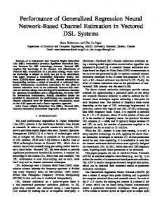
3. NN based priority assigner Scheduler structure with NN is depicted in Figure. 1.
Figure 1. Scheduler structure with NN. After testing with various possible network topologies, it is found that a 3-layer NN with topology 4 15 1 (one input layer with four inputs, one hidden layer with fifteen neurons, and one output layer with one output) is a suitable one with a learning rate 0.4 shown in Figure.2.
Figure 2. A 3-layer Backpropagation NN with four input parameters. The selected NN is trained until its Mean Squared Error (MSE) is reduced to a value less than10%. Four parameters are used as inputs to the NN: (1) Si, stay_time of job i, (2) Ti, duration of job i, (3) Di, deadline of job i, and (4) Li, critical_type of
258
-
If Li (very critical) and Ti ((≥ not less) and Si (very less) then Pi α (((Di and Li) and (1/ Ti)) or Si).
max[i] += T[j]; } } max[0] = FT; for (i=0; i < m; i++) { if(FT < max[i]) FT = max[i];} c. For optimal schedule:
There are 75 different inputs and their respective output patterns created based on the mentioned criteria.
4. Backpropagation Algorithm with Greedy Alignment Procedure
n
if ( (
i =1
Details of the procedure used in this paper are given below: 1.
2.
3. 4.
5. 6.
7.
∑ Ti) / m == FT)
return Optimal schedule; else if ( (
Backpropagation algorithm Backpropagation algorithm is used to train the NN for job priorities; P is the set of n priority values, {P1, P2, …,Pn} from the NN for n jobs. Job ordering Let J is the set of n jobs ordered with respect to their priority, {P1 ≥ P2 ≥ …≥Pn}, so that the job order is; {J1 ≥ J2 ≥ …≥Jn}. Declarations Let T is the set of n non-negative values indicate job duration, {T1, T2, …,Tn}. Let M is the set of m machines ordered based on their capacity, M1 > M2 >….> Mn. M1 = M2 = ….= Mn = 0 {initialize all machines) n = total jobs in the queue and m = no. of available machines.
n
∑ Ti) / m < FT) i =1
return Feasible schedule ; else return No Schedule; } 8.
Wait for next set of n jobs and m machines.
The relationship between machine size and job size is that machine size must be a proper divisor of job size. The optimality of the scheduler can be expressed by the theorem [8]: Theorem: Every feasible schedule has FT not earlier than the time (
n
∑ Ti) / m ,
where Ti is
i =1
duration of jobs and m is number of machines. A schedule with finishing time FT, the m machines can use a total of at most m.FT time units. During this time, for executing all jobs
Greedy procedure if (n > m)
n
∑ Ti
requires
{ a. For alignment : if (n%m ==0 ) { for (i=0; i < m; i++) { for (j=i; j < n; j+=m) T[j] Æ M[j]; } } b. For FT calculation: for (i=0; i < m; i++) { for (j=i; j < n; j+=m)
time
units.
Hence,
i =1
n
n
i =1
i =1
∑Ti) or FT > (∑ Ti) / m , is a feasible
m.FT > (
schedule.
n
∑Ti) / m,
If any FT= (
i =1
schedule must be an optimal one.
259
then that
Table 2 shows scheduled result of 8 jobs with 2 machines M1 and M2. Two adjacent priority jobs are given to two adjacent capacity machines at a time. Scheduled jobs are shown along with their durations (which are given in bracket). The scheduler provides a feasible result (FT is 1.6). Similarly, Table 3 shows scheduled result of 8 jobs with 4 machines M1, M2, M3 and M4. Four adjacent priority jobs are given to four adjacent capacity machines at a time. Scheduled jobs are shown along with their durations (which are given in bracket). FT of the feasible schedule is 1.0.
The main task of the greedy procedure is to allocate prioritized jobs onto relevant machines with feasible FT. The deadline parameter used in this paper is just for estimating the priority of a job. Once the priorities are assigned, validity of the deadline is irrelevant with respect to the scheduler.
5. Simulation Results The proposed scheduler is written in DOS based C++. Simulations are made to analyze the proposed scheduler in terms of their FT. Based on the mentioned optimality condition, the scheduler displays the schedules after providing various jobs and machine sizes. There are three sets of simulations made; 8 jobs with 2 and 4 machines, 12 jobs with 3 and 4 machines and finally 15 jobs with 3 and 5 machines. Details of the simulations carried out are given below:
Table 2. Schedule result with two machines (M1 and M2). M1 M2
M1 M2 M3 M4
Ti 0.50 0.30 0.40 0.30 0.40 0.20 0.20 0.60
Li 0.50 0.70 0.40 0.80 0.80 0.80 0.20 0.80
J5 (0.4) J6 (0.2) J8 (0.6) J4 (0.3)
J7 (0.2) J1 (0.5) J3 (0.4) J2 (0.3)
FT = 1.0 (Feasible Schedule)
5.2. Twelve jobs with three and four machines Table 4 shows unseen input dataset and their respective output Pi by the NN. Job J12 shows highest priority and job J10 shows next to highest priority. For J12, Si is very high, Di is very strong, Ti is weak and Li very critical. Similarly, job J11 is the lowest priority one; Si is not less, Di is weak, Ti is less and Li is simple. From the given input values and the respective priority values, it is confirmed that the NN assign priority for each job exactly based on the embedded priority criteria (which is explained in the section 3).
Table 1. Output of the priority assigner with eight jobs and input parameters. Di 0.60 0.60 0.80 0.80 0.70 0.90 0.90 0.80
J3(0.4) J2(0.3)
Table 3. Schedule result with four machines (M1, M2, M3 and M4).
Table 1 shows 1unseen input dataset and their respective output Pi by the NN. Job J5 shows highest priority and job J6 shows next to highest priority. For J5, Si is very less, Di is strong and Li almost very critical. Similarly, job J2 is the lowest priority one; Si is less, Di is not weak, Ti is less and Li is critical. From the given input values and the respective priority values, it is confirmed that the NN assign priority for each job exactly based on the embedded priority criteria (which is explained in the section 3).
Si 0.40 0.30 0.20 0.40 0.10 0.50 0.60 0.10
J8(0.6) J7(0.2) J4(0.3) J1(0.5)
FT = 1.6 (Feasible Schedule)
5.1. Eight jobs with two and three machines
Ji J1 J2 J3 J4 J5 J6 J7 J8
J5(0.4) J6(0.2)
Pi 0.114296 0.031031 0.093496 0.533812 0.817793 0.772682 0.139555 0.744369
260
Table 4. Output of the priority assigner with twelve jobs and input parameters.
5.2. Fifteen jobs with three and five machines
Ji J1 J2 J3 J4 J5 J6 J7 J8 J9 J10 J11 J12
Table 7 shows unseen input dataset and their respective output Pi by the NN. Job J12 shows highest priority and job J10 shows next to highest priority. For J12, Si is very high, Di is very strong, Ti is weak and Li very critical. Similarly, job J11 is the lowest priority one; Si is not less, Di is weak, Ti is less and Li is simple. From the given input values and the respective priority values, it is confirmed that the NN assign priority for each job exactly based on the embedded priority criteria.
Si 0.40 0.30 0.20 0.40 0.10 0.50 0.60 0.10 0.30 0.40 0.60 0.80
Di 0.60 0.60 0.80 0.80 0.70 0.90 0.90 0.80 0.70 0.80 0.40 0.90
Ti 0.50 0.30 0.40 0.30 0.40 0.20 0.20 0.60 0.60 0.20 0.20 0.30
Li 0.50 0.70 0.40 0.80 0.80 0.80 0.20 0.80 0.60 0.70 0.30 0.90
Pi 0.114296 0.031031 0.093496 0.533812 0.817793 0.772682 0.139555 0.744369 0.191736 0.858335 0.001740 0.955539
Table 7. Output of the priority assigner with fifteen jobs and input parameters. Ji J1 J2 J3 J4 J5 J6 J7 J8 J9 J10 J11 J12 J13 J14 J15
Table 5 shows scheduled result of 12 jobs with 3 machines M1, M2 and M2. Three adjacent priority jobs are given to three adjacent capacity machines at a time. The scheduler provides a feasible result (FT is 1.5). Similarly, Table 6 shows scheduled result of 12 jobs with 4 machines M1, M2, M3 and M4. Four adjacent priority jobs are given to four adjacent capacity machines at a time. The scheduler provides a feasible result (FT is 1.4). Table 5. Schedule result with three machines (M1, M2, and M3).
Si 0.40 0.30 0.20 0.40 0.10 0.50 0.60 0.10 0.30 0.40 0.60 0.80 0.70 0.40 0.30
Di 0.60 0.60 0.80 0.80 0.70 0.90 0.90 0.80 0.70 0.80 0.40 0.90 0.80 0.90 0.90
Ti 0.50 0.30 0.40 0.30 0.40 0.20 0.20 0.60 0.60 0.20 0.20 0.30 0.20 0.70 0.80
Li 0.50 0.70 0.40 0.80 0.80 0.80 0.20 0.80 0.60 0.70 0.30 0.90 0.30 0.80 0.80
Pi 0.114296 0.031031 0.093496 0.533812 0.817793 0.772682 0.139555 0.744369 0.191736 0.858335 0.001740 0.955539 0.849658 0.669770 0.509433
Table 8 shows scheduled result of 15 jobs with 3 machines M1, M2 and M2. Three adjacent priority jobs are given to three adjacent capacity machines at a time. The scheduler provides a feasible result (FT is 2.4). Similarly, Table 9 shows scheduled result of 12 jobs with 5 machines M1, M2, M3, M4 and M5. Five adjacent priority jobs are given to five adjacent capacity machines at a time. The scheduler provides a feasible result (FT is 1.5).
FT = 1.5 (Feasible Schedule) Table 6. Schedule result with four machines (M1, M2, M3 and M4). M1 J12 (0.3) J8 (0.6) J1 (0.5) M2 J10 (0.2) J4 (0.3) J3 (0.4) M3 J5 (0.4) J9 (0.6) J2 (0.3) M4 J6 (0.2) J7 (0.2) J11 (0.2) FT = 1.4 (Feasible Schedule)
261
[4] Sauer, “Knowledge Based Scheduling in PROTOS”, Proceedings of IMACS World Congress on Computation and Applied Mathematics, Dublin, 1991. [5] W. Slany, “Scheduling as a fuzzy multiple criteria optimization problem”, CD-Technical Report 94/62, Technical University of Vienna, 1994. [6] V. B. Rao and H. V. Rao, Neural Networks & Fuzzy logic, BPB Publications, 1996. [7] K. G. Anilkumar and T. Tanprasert, “Neural Network Based Priority Assignment for Job Scheduler”, AU Journal of Technology, ABAC, vol.9, ISSN: 1513-0886, 2006. [8] S. Stinson, An Introduction to the Design and Analysis of Algorithms, Cambridge Press, 1980.
Table 8. Schedule result with three machines (M1, M2, and M3).
FT = 2.4 (Feasible Schedule) Table 9. Schedule result with five machines (M1, M2, M3, M4 and M5). M1 J12(0.3) J8(0.6) J7(0.2) M2 J10(0.2) J14(0.7) J1(0.5) M3 J13(0.2) J4(0.3) J3(0.4) M4 J5(0.4) J15(0.8) J2(0.3) M5 J6(0.2) J9(0.6) J11(0.2) FT = 1.5 (Feasible Schedule)
6. Conclusion The proposed scheduler schedules jobs based on their priority. It is confirmed that priorities assigned by the NN are exactly accurate with respect to the given priority criteria. Machines used in this paper are ordered based on their capacity prior to each schedule. Simulations of the scheduler with various jobs and machine sizes have shown respective feasible schedules. Even though there are no optimal results from the proposed scheduler, schedules with more machines produce better results than schedules with fewer machines (job size > machines).
7. Acknowledgements The support of the Montfort Brothers of St. Gabriel, Assumption University, is gratefully appreciated.
8. References [1] D. Dubois, H. Fargier, and H. Prade, “Fuzzy constraints in job-shop scheduling,” J.Intell. Manufacturing, vol.6, pp.215-234, 1995. [2] J.J Hopefield and D.W. Tank, “Neural computation of decisions in optimization problems,” Biol. Cybern., vol.52, pp. 141-152, 1985. [3] T. Kohonen, Self-Organization and Associative Memory, Springer-Verlag, Berlin 1984.
1
Input combinations which are not included in the initial training set of the NN are considered as ‘unseen’.
262