Neural Network Modeling of Substituent Constants on

ISSN 00125008, Doklady Chemistry, 2010, Vol. 431, Part 1, pp. 85–88. © Pleiades Publishing, Ltd., 2010. Original Russian Text © M.N. Kurilo, P.V. Karpov, I.I. Baskin, V.A. Palyulin, N.S. Zefirov, 2010, published in Doklady Akademii Nauk, 2010, Vol. 431, No. 3, pp. 347–350.

CHEMISTRY

Neural Network Modeling of Substituent Constants on the Basis of Fragmental Descriptors M. N. Kurilo, P. V. Karpov, I. I. Baskin, V. A. Palyulin, and Academician N. S. Zefirov Received September 29, 2009

DOI: 10.1134/S0012500810030067

Predicting the properties of new organic com pounds is an important component of a study aimed at searching for new promising structures with desired properties. The studies of relationships between the structure and activity/properties of organic com pounds (QSAR/QSPR) were initiated more than half a century ago. To describe the effect of structural changes on the properties, L. P. Hammett proposed some parameters, referred to as Hammett constants [1], which are actively used to the present day. The development of basic concepts and principles of theo retical organic chemistry, such as inductive and reso nance effects, quantitative interpretation of steric effects near the reaction center, and elucidation of organic reaction mechanisms, has been inspired by correlation equations based on the Hammett con stants [2].

for constructing nonlinear dependences. They have been successfully used for predicting the boiling points, viscosity, density, and other properties of organic compounds [8]. The present work is aimed at constructing predic tive neural network QSPR models for a series of sub stituent constants and verifying the applicability of the predicted constants to QSAR studies (i.e., for hierar chical QSAR). Various methods have been used for predicting the substituent constants, beginning with empirical parameters of organic structures and ending with complicated quantumchemical calculations. Rela tionships between topological indices and steric parameters—molecular volume and refraction, as well as empirical steric constants Es—have been obtained in the framework of the topological approach [3]. A threelayer fully connected neural network was used for predicting the constants in the Hansch equa tion [4]. To predict the π and MR constants, the Kier– Hall Estate descriptors were calculated. The correla tion coefficient for the test set was 0.92 and 0.96, respectively. In addition, the field F (r = 0.85) and res onance R (r = 0.84) electronic constants were pre dicted using a set of modified molecular descriptors.

Nowadays, there are a large number of substituent constants, used for optimizing desired properties. Nevertheless, the vast majority of such constants are experimental and their values are unknown for most possible substituents. Modern quantumchemical methods can be used for calculating some constants; however, for processing large databases, these methods are still too timeconsuming and inefficient and often do not afford required accuracy. At the same time, a host of QSPR procedures for predicting substituent constants are available in the literature. They are based on different types of descriptors and algorithms of constructing correlation models [3–7].

Cherkasov and Jonsson [5] suggested an additive model (r = 0.98) which implies that the steric and inductive effects of a substituent are determined by the overall effect of its constituting atoms as a logarithmic dependence of the sum of squared ratios of atomic radii and the distances from the centers of atoms to the reaction site.

It is evident that the complexity of the actual phys ical picture of the substituent effect on the molecule core, expressed through substituent constants, casts some doubt on the existence of simple linear depen dences of these constants on more significant parame ters of organic compounds, such as properties of atoms constituting the structure, polarizability, permittivity, and others. Such a dependence should be nonlinear, and artificial neural networks are one of the best tools

The use of quantumchemical descriptors made it possible for the QSPR model parameters to approxi mate real physical representations at the molecular level. In [6], the theoretically calculated electrostatic potentials of monosubstituted benzene rings were suc cessfully used as descriptors in linear regression analy sis (r = 0.99). The frontier orbital theory was used for studying the electronic effects of substituents [7]. The correlation coefficient obtained with the use of quan

Moscow State University, Moscow, 119991 Russia 85

86

KURILO et al.

Statistical parameters of constructed QSPR models R Constant π MR F R σm σp σI σL – σp + σp R– R+ Es σ* σP

Constant description [2, 11] Lipophilicity Molar refraction Swain–Lupton field constant Swain–Lupton resonance constant Classical Hammett constants (meta) Classical Hammett constants (para) Hammett inductive constant Inductive constant determined by Charton Nucleophilic σ constant Electrophilic σ constant Swain–Lupton nucleophilic constant Swain–Lupton electrophilic constant Taft steric constant Taft inductive constant Phosphorus σ constant

N 173 342 296 295 352 403 460 129 154 146 95 60 94 381 57

n 58 86 74 51 84 88 95 72 51 40 31 22 25 47 14

RMSE

x 3 2 4 2 6 4 9 6 6 6 5 5 4 3 3

T

V

P

T

V

P

0.98 0.99 0.97 0.96 0.88 0.98 0.91 0.99 0.99 0.97 0.96 0.97 0.94 0.97 0.87

0.94 1.00 0.79 0.86 0.64 0.93 0.87 0.95 0.97 0.71 0.98 1.00 0.96 0.95 0.90

0.90 0.98 0.85 0.84 0.95 0.92 0.81 0.90 0.84 0.67 0.84 0.73 0.89 0.93 0.87

0.27 0.10 0.06 0.06 0.14 0.07 0.09 0.02 0.07 0.26 0.12 0.11 0.36 0.30 0.28

0.34 0.11 0.14 0.12 0.18 0.14 0.12 0.09 0.18 0.41 0.24 0.20 1.11 0.48 1.01

0.40 0.15 0.10 0.10 0.08 0.15 0.17 0.28 0.25 0.47 0.38 0.48 0.53 0.57 0.24

Note: N is the number of substituents, n is the number of descriptors, x is the number of hidden neurons.

tumchemical and topological descriptors was 0.98 for the set of 150 substituents. In contrast to the above methods, we suggest using fragmental descriptors as parameters for modeling. As shown in [9], any molecular descriptor can be repre sented as a combination (linear or polynomial) of frag mental descriptors. Coupled with neural network modeling, fragmental descriptors were previously used by us for constructing statistically significant models for physicochemical properties of organic molecules [8, 10]. To construct models, we formed a database on the basis of handbook [11]. The database contains infor mation on 1256 substituents and their constants. It is worth noting that the substituents contained in the database are structurally very diverse. In addition to common substituents (aliphatic, aromatic, heterocy clic, etc.), there are organometallic structures con taining B, Ge, As, In, Sn, Te, and Hg. Organosele nium and organosilicon substituents are rather widely presented in the database. On the one hand, this het erogenicity of the set can impair regression results but, on the other hand, it can enlarge the applicability of the model as compared with the models based on more homogeneous sets. The fragmental descriptors were calculated for all compounds of the database with the use of the FRAG MENT block [8] built into the NASAWIN software [12]. Fragments generated by the program contain chains of 1 to 15 atoms, rings of 3 to 15 atoms, three branched fragments, bicyclic fragments of 6 to

15 atoms in various combinations, and tricyclic frag ments of 12 to 15 atoms in various combinations. The value of a fragmental descriptor is the number of occurrences of the corresponding subgraph in the molecular graph; i.e., the fragmental descriptor shows the number of the corresponding substructures in the chemical structure. The FRAGMENT block provides a redundant description of the structure; however, since neural network models are prone to overtraining, it is necessary to select the most significant descrip tors. For selection, the fast stepwise multiple linear regression (FSMLR) method was used [13]. For constructing QSPR models, the threelayer fully connected feedforward neural network with the n–x–1 architecture was used: n is the number of neu rons in the input layer corresponding to the number of selected descriptors; the number of hidden neurons in the inner layer (x) varied from two to nine to achieve the best model quality/complexity ratio; the output layer consisted of one neuron corresponding to the predicted property. The network was learned by the backpropagation learning algorithm. To do this, the initial set of compounds for each modeled property was divided into the training, validation, and predic tion sets. This partition prevents network overtraining. Neural network modeling was performed with the NASAWIN program package [12]. Statistically significant QSPR models were con structed for 15 constants. In all cases, the number of hidden neurons was optimized. Statistical model parameters, namely, the correlation coefficient R and DOKLADY CHEMISTRY

Vol. 431

Part 1

2010

NEURAL NETWORK MODELING OF SUBSTITUENT CONSTANTS 2

4.5 π

0

3.5

–2

2.5

–4

1.5

–6

–4 –2

0

2

MR

1.5

1.5

R

0.75

2.5 3.5

1.5

σm

1.0

1.0

1.0

0.5

0.5

0

0

0

0

0.5

1.0 –0.5

0

0.5

1.0

1.5 –0.5

1.5 σI

0.7

Calculation

0.1 0

–0.5

0.5

1.0

1.5

σp+

0.5

1.0

0.5

1.0

1.5

σp–

0.4

0.7

–0.5 0.5

R–

0

1.5

R+

0

0 –0.5

–0.50

–0.5 –0.50 0.25

1.00

–1.0

Es

6

–1.5

4

–2.5

2

–3.5

0

–4.5

0.1

0.5

0.25

–0.5

0

0

–0.2 1.0

–1.25

σp

0.5

0

1.00

1.0

0.4

0.5

0.75

1.5

σL

1.0

0.25

4.5 –0.25

0.5

–0.5

F

0.25

0.5

1.5

–1.0

87

–2

–3.5–2.5–1.5–0.5

–0.5

0

1.0 –1.0

0.5

0.5

σ*

–0.5

0

0.5

σP

0 –0.5 –1.0 0

2 4 Experiment

6

–1.5

–1.0 –0.5

0

0.5

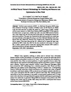
Correlation between predicted and experimentally measured substituent constants. (䉬) Training, ( ) validation, and (䉭) predic tion sets.

the rootmeansquare error RMSE for the training (T), validation (V), and prediction (P) sets, as well as the optimal number of hidden neurons are listed in the table. The corresponding plots demonstrating the correlation between the predicted and experi DOKLADY CHEMISTRY

Vol. 431

Part 1

2010

mentally measured substituent constants are shown in the figure. Most of the constructed models have a satisfactory predictive power. The highest correlation coefficients

88

KURILO et al.

were obtained for the molar refraction MR (0.99, 1.00, 0.98 for the training, test, and independent prediction sets, respectively), which is due to the best accuracy of the experimental data for MR. As expected, the lowest correlation coefficients (0.87, 0.90, 0.87) were obtained for σP available only for a small set of substit uents. It is worth noting that the set for R+ contains only three extra substituents, but the correlation coef ficients (0.97, 1.00, 0.73) are considerably higher than those for σP, which is presumably due to the higher homogeneity of the set for the electrophilic resonance constant. Thus, we constructed neural network models for 15 substituent constants on the basis of fragmental descriptors. All models demonstrated satisfactory pre dictive power for the independent test sets. The con stants calculated on the basis of these models can be used as descriptors for optimization of biological activity in the framework of hierarchical (multilevel) QSAR/QSPR [14]. REFERENCES 1. Hammett, L.P., J. Am. Chem. Soc., 1937, vol. 59, pp. 96–103. 2. Hansch, C., Leo, A., and Taft, R., Chem. Rev., 1991, vol. 91, pp. 165–195. 3. Cherkasov, A.R., Galkin, V.I., and Cherkasov, R.A., Usp. Khim., 1996, vol. 65, pp. 695–711. 4. TingLan Chiu and SungSau, So, J. Chem. Inf. Com put. Sci., 2004, vol. 44, pp. 147–153.

5. Cherkasov, A. and Jonsson, M., J. Chem. Inf. Comput. Sci., 1998, vol. 38, pp. 1151–1156. 6. Galabov, B., Ilieva, S., and Schaefer, H., J. Org. Chem., 2006, vol. 71, pp. 6382–6387. 7. Sullivan, J., Jones, D., and Tanji K., J. Chem. Inf. Com put. Sci., 2000, vol. 40, pp. 1113–1127. 8. Artemenko, N.V., Baskin, I.I., Palyulin, V.A., and Zefirov, N.S., Dokl. Chem., 2001, vol. 381, nos. 1–3, pp. 317–320 [Dokl. Akad. Nauk, 2001, vol. 381, no. 2, pp. 203–206]. 9. Baskin, I.I., Skvortsova, M.I., Stankevich, I.V., and Zefirov, N.S., J. Chem. Inf. Comput. Sci., 1995, vol. 35, pp. 527–531. 10. Artemenko, N.V., Baskin, I.I., Palyulin, V.A., and Zefirov, N.S., Izv. Akad. Nauk, Ser. Khim., 2003, pp. 19–28. 11. Hansch, C., Leo, A., and Hoekman, D., Exploring QSAR. Hydrophobic, Electronic, and Steric Constants, Washington: ACS, 1995. 12. Baskin, I.I., Halberstam, N.M., Artemenko, N.V., Palyulin, V.A., and Zefirov, N.S., in EuroQSAR 2002. Designing Drugs and Crop Protectants: Processes, Prob lems and Solutions, Melbourne: Blackwell, 2003, pp. 260–263. 13. Zhokhova, N.I., Baskin, I.I., Palyulin, V.A., Zefir ov, A.N., and Zefirov, N.S., Dokl. Chem., 2007, vol. 417, part 2, pp. 282–284 [Dokl. Akad. Nauk, 2007, vol. 417, no. 5, pp. 639–641]. 14. Baskin, I.I., Zhokhova, N.I., Palyulin, V.A., Zefi rov, A.N., and Zefirov, N.S., Dokl. Chem., 2009, vol. 427, part 1, pp. 172–175 [Dokl. Akad. Nauk, 2009, vol. 427, no. 3, pp. 335–339].

DOKLADY CHEMISTRY

Vol. 431

Part 1

2010