Neural network parametrization of spectral functions from hadronic tau ...

hep-ph/0401047 UB–ECM–PF 04/01

arXiv:hep-ph/0401047v1 9 Jan 2004

Neural network parametrization of spectral functions from hadronic tau decays and determination of QCD vacuum condensates Juan Rojo and Jos´ e I. Latorre Departament d’Estructura i Constituents de la Mat`eria, Universitat de Barcelona, Diagonal 647, E-08028 Barcelona, Spain

Abstract The spectral function ρV −A (s) is determined from ALEPH and OPAL data on hadronic tau decays using a neural network parametrization trained to retain the full experimental information on errors, their correlations and chiral sum rules: the DMO sum rule, the first and second Weinberg sum rules and the electromagnetic mass splitting of the pion sum rule. Nonperturbative QCD vacuum condensates can then be determined from finite energy sum rules. Our method minimizes all sources of theoretical uncertainty and bias producing an estimate of the condensates which is independent of the specific finite energy sum rule used. The results for the central values of the condensates hO6 i and hO8 i are both negative.

January 2004

1

1

Introduction

As the predictions of QCD become increasingly precise and more high quality data is available, the theoretical uncertainties associated with the analysis of the data are often found to be dominant and thus have come under increasing scrutiny. In this work we continue previous efforts [1, 2] to optimize the analysis of the information contained in the experimental data, taking into account errors and correlations, while introducing the smallest possible theoretical bias. We consider the determination of the QCD vacuum condensates hO6 i , hO8 i and higher dimensional condensates, which in principle can be extracted in a theoretically solid and experimentally clean way from the hadronic decays of the tau lepton. In practice, however, the situation is far from satisfactory, as revealed by the lack of stability of the value of the nonperturbative condensates obtained from this process by different procedures. The main source of difficulties can be traced to the fact that conventional extractions of the QCD vacuum condensates from hadronic tau decays involve convolutions of the difference v1 (s) − a1 (s) of the isovector vector and axial vector spectral functions, which is a purely nonperturbative quantity, that does not converge to the perturbative result (these spectral functions are degenerate within perturbation theory) at energies s ≤ Mτ2 and moreover has large uncertainties in the high s region. To obtain a reliable value for the nonperturbative condensate, some convergence method must be applied, implying that the error on the condensates gets tangled with uncertainties within the theoretical assumptions and subject therefore to a variety of sources of theoretical bias. This is a consequence of the fact that the kinematics of the hadronic tau decays constrains the range of energies in which we can evaluate the spectral functions. The main difficulty is that any method to estimate non-perturbative condensates exploits the shape of the spectral functions near and beyond the boundary of the region where the data is available. Final results are then subject to systematics errors associated to the extrapolation of data as well as the way global theoretical constraints, e. g. Weinberg sum rules, are imposed. In this paper, we approach the determination of nonperturbative condensates, in a way which tries to bypass these difficulties, by combining two techniques. First, a novel bona fide method to take into account experimental errors was proposed and implemented in the context of analysis of Deep Inelastic Scattering data to produce a probability measure in the space of deep inelastic structure functions by means of neural networks [3]. Here, we adapt this method to the parametrization of spectral functions. The second technique we use refines the training of neural networks so as to implement the constraints that represent the QCD chiral sum rules in our neural network parametrization of the spectral function v1 (s) − a1 (s). The representation of the probability density given in Ref. [3] takes the form of a set of neural networks, trained on an ensemble of Monte Carlo replicas of the experimental data, which reproduce their probability distribution. The parametrization is unbiased in the sense that neural networks do not rely on the choice of an specific functional form, and it interpolates between data points, imposing smoothness constraints in a controllable way. Information on experimental errors and correlations is incorporated in the Monte Carlo sample. Errors on physical quantities and correlations between them can then be determined without the need of linearized error propagation. Our final parametrization combines all the available experimental information, as well as constraints from different convolutions of the data, i.e. chiral sum rules, must verify. In this way statistical errors can be estimated and the loss of accuracy due to the extrapolation outside the kinematical region where the data is available is also analyzed. 2

Hence, we can obtain a determination of the QCD vacuum condensates which is unbiased with respect to the parametrization of the spectral function and the error and correlations propagation. We also try to keep under control all sources of uncertainty related to the method of analysis, and estimate their contribution to the total error. This gives us a determination of the nonperturbative condensates, and simultaneously illustrates the power of a method of analysis based on direct knowledge of a probability density in a space of functions. This paper is organized as follows: in section 2 we review theoretical tools used in the analysis of non-perturbative effects in hadronic tau decays; in section 3 we present the experimental data that is used in our analysis and in section 4 we introduce the neural network parametrization of spectral functions. Section 5 contains the details and results of our extractions of the vacuum condensates: we explain our choice of training parameters, our error estimations and the consistency tests that we performed; finally section 6 summarizes our conclusions.

2

Spectral functions and hadronic tau decays

The tau particle is the only lepton massive enough to decay into hadrons. Already before its discovery, it was predicted to be important for the study of hadronic physics [4], a study that has been performed extensively at the LEP accelerator. Its semileptonic decays are therefore an ideal tool for studying the hadronic weak currents under clean conditions, both theoretically and experimentally, thanks to the high quality data from LEP. In this first section we will briefly introduce the theoretical foundations that form the basis of the QCD analysis of hadronic tau decays. There exists a huge literature on tau hadronic physics to which the interested reader is directed (see for instance Ref. [5] and references therein). Spectral functions are the observables that give access to the inner structure of hadronic tau decays. As parity is maximally violated in τ decays, the spectral functions will have both vector and axial vector contributions. As spontaneous chiral symmetry breaking is a nonperturbative phenomena, this spectral functions are degenerate in perturbative QCD with massless light quarks, so any difference between vector and axial-vector spectral functions is necessarily generated by non-perturbative dynamics, that is, long distances resonance phenomena, being the most relevant the ρ(770) and the a1 (1260) in the vector and axial vector channels respectively. Therefore, the difference of these spectral functions is generated entirely from nonperturbative QCD dynamics, and provides a laboratory for the study of these perturbative contributions, which have resulted to be small and therefore difficult to measure in other processes where the perturbative contribution dominates. An accurate extraction of the QCD vacuum condensates is not only important by itself but also has many important phenomenological applications, for example in the evaluation of matrix elements in weak decays [6]. The ALEPH collaboration at LEP measured [7, 8] these spectral functions from hadronic tau decays with great accuracy, providing an excellent source of precision analysis of nonperturbative effects. As it is well known [10], the basis of the comparison of theory with data is the fact that unitarity and analyticity connect the spectral functions of hadronic tau decays to the imaginary part of the hadronic vacuum polarization, Πµν ij,U (q) ≡

Z

D





E

d4 x eiqx 0|T Uijµ (x)Uijν (0)† |0 ,

(1)

of vector Uijµ ≡ Vijµ = q¯j γ µ qi or axial vector Uijµ ≡ Aµij = q¯j γ µ γ5 qi color singlet quark currents in corresponding quantum states. After Lorentz decomposition is used to separate the correlation 3

function into its J = 1 and J = 0 components, 



(1)

(0)

µν 2 µ ν Πij,U (q 2 ) + q µ q ν Πij,U (q 2 ) , Πµν ij,U (q) = −g q + q q

for non-strange quark currents one identifies (1)

ImΠu¯d,V /A (s) =

1 v1 /a1 (s) . 2π

(2)

(3)

This relation allows us to implement all the technology of QCD vacuum correlation functions to hadronic tau decays, and provides the basis of the comparison of theory with data. The basic tool to study in a systematic way the power corrections introduced by nonperturbative dynamics is the operator product expansion. Since the approach of Ref. [13], the operator product expansion (OPE) has been used to perform calculations with QCD on the ambivalent energy regions where nonperturbative effects come into play but still perturbative QCD is relevant. In general, the OPE of a two point correlation function Π(J) (s) takes the form [10] X X 1 C (J) (s, µ) hO(µ)i , (4) Π(J) (s) = D/2 (−s) dimO=D D=0,2,4,... where the arbitrary parameter µ separates the long distance nonperturbative effects absorbed into the vacuum expectation elements hO(µ)i, from the short distance effects which are included in the Wilson coefficient C (J) (s, µ). The operator of dimension D = 0 is the unit operator (perturbative series), and we are interested in the dimension D ≥ 6 operators. What is relevant for us is that D = 6 is the first non-vanishing non-perturbative contribution, in the limit of massless light quarks, to the v1 (s) − a1 (s) spectral function and, moreover, it has been shown to be the dominant one. This dominant contribution carries non-trivial four-quark dynamical effects of the form q¯i Γ1 qj q¯k Γ2 ql . Additional contributions from a mixed quark gluon condensate as well as a triple gluon condensate are assumed to be small. Therefore, this spectral function should provide a source for a clean extraction of the value of the nonperturbative contributions. Finally, we review the important paper that QCD chiral sum rules play in the analysis of this process. Sum rules have always been an important tool for studies of non-perturbative aspects of QCD, and have been applied to a wide variety of processes, from Deep Inelastic Scattering to Heavy Quark systems [14], [15]. Now we will review one of the classical examples of low energy QCD sum rules, the chiral sum rules. The application of chiral symmetry together with the optical theorem leads to low energy sum rules involving the difference of vector and axial vector spectral functions, ρV −A (s) ≡ v1 (s) − a1 (s) .

(5)

These sum rules are dispersion relations between real and absorptive parts of a two point correlation function that transforms symmetrically under SU(2)L ⊗ SU(2)R in the case of non strange currents. Corresponding integrals are the Das-Mathur-Okubo sum rule [18] 1 4π

Z

0

s0 →∞

1 fπ2 < rπ2 > ds ρV −A (s) = − FA , s 3

(6)

as well as the first and second Weinberg sum rules (WSR) [19] 1 4π 2

Z

0

s0 →∞

dsρV −A (s) = fπ2 , 4

(7)

Z

s0 →∞ 0

dssρV −A (s) = 0 ,

(8)

where in eq. (7) the RHS term comes from the integration of the spin zero axial contribution, which for massless non-strange quark currents consists exclusively of the pion pole. Finally, there is the chiral sum rule associated with the electromagnetic splitting of the pion masses [20], 1 4π 2

Z

s0 →∞

0

dss ln

4πfπ2 2 s ρ (s) = − (mπ± − m2π0 ) , V −A 2 λ 3α

(9)

where fπ = (92.4 ± 0.3) MeV [12] obtained from the decays π − → µ− ν¯µ and π − → µ− ν¯µ γ, FA = 0.0058 ± 0.00008 is the pion axial vector form factor1 obtained from the radiative decays π − → l− ν¯l γ and hrπ2 i = (0.439 ± 0.008) fm2 is the pion charge radius squared. From now on these four chiral sum rules will be denoted by SR1, SR2, SR3 and SR4 respectively. It could be argued that as long that these chiral sum rules are taken in the chiral limit, the value of the pion decay constant should be the chiral limit value, f ∼ 0.94fπ [16]. However, as long as the experimental data consists of real pions, we consider that it is more reasonable to use the real world value for the pion decay constant. When switching quark masses on, only the first WSR remains valid while the second breaks down due to contributions from the difference of non-conserved vector and axial vector currents of order m2q /s leading to a quadratic divergence of the integral. This is not numerically relevant in our analysis because we deal with finite energy sum rules, and in this case the contribution from non-zero quark masses is negligible. The QCD vacuum condensates can be determined by virtue of the dispersion relation from another sum rule, that is, a convolution of the ρV −A (s) spectral function with an appropriate weight function. Let us define the operator product expansion of the chiral correlator in the following way Π(Q2 )|V −A =

∞ X

∞ D E X 1 2 2 2 C (Q , µ ) O (µ ) ≡ hO2n+4 i . 2n+4 2n+4 2n+4 2n+4 n=1 Q n=1 Q

1

(10)

The Wilson coefficients, including radiative corrections, are absorbed into the nonperturbative vacuum expectation values, to facilitate comparison with the current literature. The analytic structure of the Π is subject to the dispersion relation 2

ΠV −A (Q ) =

Z

0

∞

ds

1 1 ImΠV −A (s) . s + Q2 π

(11)

Condensates of arbitrary dimension are simply given by hO2n+2 i = (−1)n

Z

0

s0

dssn

1 (v1 (s) − a1 (s)) , 2π 2

n≥2,

(12)

which,if the asymptotic regime has reached, should be independent of the upper integration limit for large enough s0 . As can be seen from the experimental data, errors in the large s region are very important, so large errors are expected in the evaluation of the condensates. The analysis of these sources of errors is one of our main goals in the present analysis, which will be obtained thanks to the natural capability of neural networks of smooth interpolating while implementing all the experimental information on errors and correlations. 1

Note that our definition of FA agrees with that of Ref. [7] but differs by a factor of 1/2 from that given in Ref. [12]

5

2.1

Finite energy sum rules

As long as all previous integrals have to be cut at some finite energy s0 ≤ Mτ2 , since no experimental information on v1 (s) − a1 (s) is available above Mτ2 , we must perform a truncation that competes with all other sources of statistical and systematic errors, introducing a theoretical bias which is difficult to estimate. Many techniques have been developed to deal with this finite energy integrals, leading to the so-called Finite Energy Sum Rules (FESR). The paradigmatic example is the calculation of spectral moments [21], that is weighted integrals over spectral functions. Choosing appropriate weights allows to extract the maximum information possible from the experimental data while minimizing the contribution from the region with larger errors. This techniques allow a comparison of the same quantity evaluated on one side with experimental data and on the other side with theoretical input, basically the Operator Product Expansion with perturbative QCD corrections. The general expression that takes advantage of the analyticity properties of the chiral correlators is given by Z

s0 0

(J)

ds W (s) ImΠV −A (s) =

1 2i

I

(J)

|s|=s0

ds W (s) ΠV −A (s) ,

(13)

where W (s) is an analytic function and s0 is large enough for the OPE series to converge. The LHS of eq. (13) can be evaluated using the experimental input from spectral functions as determined in hadronic tau decays, while the RHS can be evaluated using the OPE representation of the chiral correlator. Finally, a fit is performed to extract the OPE parameters from the experimental data on spectral functions. A common hypothesis in the majority of this kind of analysis is that the difference of the OPE representation for the chiral correlator from the full expression, −1 R[s0 , W ] ≡ 2πi

Z

|s|=s0

ds (ΠV −A,OP E (s) − ΠV −A (s)) W (s) ,

(14)

can be neglected. This quantity is a measure of the OPE breakdown, also known as duality violation2 . It is necessary to take into account that ΠV −A,OP E fails at least in some region of the integration contour. This was shown in Ref. [17], where it was demonstrated that the OPE representation breaks down near the timelike real s axis for insufficiently large s0 . The neglect of the duality violation component of the OPE is a key dynamical assumption and there exists several strategies to minimize its impact, as working with duality points [28] or using pinched Finite Energy Sum Rules [29], with polynomial weights that vanish at the upper integration limit. All these techniques yield different although compatible values for the hO6 i, whereas non-compatible results are obtained for higher condensates. Other types of finite energy sum rules have been used to extract the values of the condensates and other phenomenologically relevant related quantities. Borel sum rules and Gaussian sum rules [24] take advantage of certain combination of the condensates that theoretically optimize the accuracy of the extraction. Inverse moment sum rules [23] techniques make a connection between the phenomenological parameters of the QCD effective Lagrangian and the nonperturbative condensates. In section 5 we will compare our extraction of the condensates to those obtained with all these methods and argue why ours has a reasonable control of the different theoretical uncertainties. 2

For a review of the current theoretical status of the quark-hadron duality violations, see Ref. [25]

6

Our approach is different with respect to previous determinations of nonperturbative condensates. First of all, we use the smooth interpolation of the neural network to extend the range of integration, so that our determination of the condensates corresponds to the asymptotic energy region s0 → ∞. The second point is that the training method allows the incorporation of the chiral sum rules to the neural network parametrization of the spectral function, and therefore the specific weight used to determine the condensate turns out not to be relevant: different choices of weights differ by chiral sum rules that are already verified our parametrization. Therefore, the final results for the non-perturbative condensates that emerge from the neural network parametrization of the spectral function v1 (s) − a1 (s) are determined by n

hO2n+2 i = (−1)

Z

0

∞

dssn

1 (v1 (s) − a1 (s)) 2π 2

n≥2.

(15)

In the next sections will be argued why this choice is the most reasonable one, showing that all relevant constraints are verified.

3

Experimental data

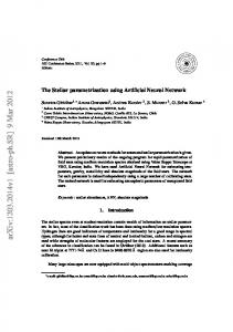
Since the relevant spectral function for the determination of the condensates is the v1 (s) − a1 (s) spectral function, we need a simultaneous measurement of the vector and axial-vector spectral functions. Data from the ALEPH Collaboration [7], [8] and from the OPAL collaboration [9] will be used, which provide a simultaneous determination of the vector and axial vector spectral functions in the same kinematic region and also provide the full set of correlated uncertainties for these measurements. Although the ALEPH data is of a higher quality due to the smaller errors, see fig. (1), the input from OPAL is complementary and will provide a cross check for our extractions of the nonperturbative condensates. There exists additional data on spectral functions coming from electron-positron annihilation, but their quality is lower than the data from hadronic tau decays and will be ignored here. ALEPH experimental data consists on the invariant square-mass spectra for both the vector+axial vector and vector-axial vector components, that are related to the spectral functions by a kinematic factor and a branching ratio normalization Mτ2 B(τ − → V − /A− ντ ) dNV /A v1 (s)/a1 (s) ≡ 6|Vud|2 SEW B(τ − → e− ν¯e ντ ) NV /A ds

"

s 1− 2 Mτ

!

2s 1− 2 Mτ

!#−1

.

(16)

Altogether our parametrization is based on Ndat = 61 experimental points for ALEPH, although the full experimental data consists in 70 points uniformly distributed between 0 and 3.5 GeV2 , because only points with s ≤ Mτ2 = 3.16 GeV2 are physically meaningful, and before this kinematic threshold is reached the invariant mass-squared spectrum vanishes due to phase-space suppression. For OPAL the data sample is a bit larger, Ndat = 97, with the (exp) same restrictions as in the ALEPH case. Henceforth, ρV −A,i will denote the i-th data point ρV −A (si ) ≡ v1 (si ) − a1 (si ). Figure (3) shows the experimental data used together with diagonal errors. Note that errors are small in the low and middle s regions and that they become larger as we approach the tau mass threshold. The last points are almost zero in the invariant mass spectrum, and are only enhanced in the spectral functions due to the large kinematic factor for s near Mτ2 , so special care must be taken with the physical relevance of these points. 7

OPAL data 2.5

2

2

1.5

1.5 v_1(s)-a_1(s)

v_1(s)-a_1(s)

ALEPH data 2.5

1

1

0.5

0.5

0

0

-0.5

-0.5

0

0.5

1

1.5 s [GeV^2]

2

2.5

3

0

0.5

1

1.5 s [GeV^2]

2

2.5

3

Figure 1: Experimental data for v1 (s) − a1 (s) spectral function from the ALEPH (left) and OPAL (right) collaborations. Note that the errors are smaller in the ALEPH data but OPAL central values are nearer to the expected zero value at large s.

It is clear that the vanishing of the spectral function is not reached for s ≤ Mτ2 and must be enforced artificially on the parametrization we are constructing, that is we must device a technique to impose the asymptotic constraint that at high s this spectral function vanishes. The method we use takes advantage of the smooth, unbiased interpolation capability of the neural network: artificial points are added to the data set with adjusted errors in a region where s is high enough that the ρV −A (s) spectral function should vanish. Once these artificial points are included, in a way to be discussed later, the neural network will smoothly interpolate between the real and artificial data points, also taking into account the constraints of the sum rules, as explained below. The experimental data points are highly correlated, because the majority of the covariance matrix is composed of nonzero entries, so it is therefore crucial to take into account all their correlations, which are specially relevant in the high s region. This is important because this region dominates the sum rule, eq. (12), that determines the vacuum condensates. As we shall discussed shortly, correlated errors are incorporated as a measure on the space of neural network parametrizations of the spectral functions using Monte Carlo statistical replicas of the experimental data.

4

Neural network parametrization

Ideally, a parametrization of spectral functions must incorporate all the information contained in the experimental measurements, i.e. their central values, their statistical and systematic errors and their correlations, furthermore, it must interpolate between them without introducing any bias. We will follow the method of Ref. [3], where an unbiased extraction of the probability measure in the space of structure functions of deep-inelastic scattering is performed, based on a coordinated use of Monte Carlo generation of data and neural network fits.

8

4.1

Probability measure in the space of spectral functions

The experimental data gives us a probability measure in an Ndat dimensional space, assumed to be multigaussian. In order to extract from it a parametrization of the desired structure function we must turn this measure into a measure P [ρV −A ] in a space of functions. Once such a measure is constructed, the expectation value of any observable F [ρV −A (s)] can be found by computing the weighted average hF [ρV −A (s)]i =

Z

DρV −A F [ρV −A (s)] P [ρV −A ] .

(17)

Errors and correlations can also be obtained from this measure, by considering higher moments of the same observable with respect to the probability distribution. The determination of an infinite-dimensional measure from a finite set of data points is an ill-posed problem, unless one introduces further assumptions. In the approach of Ref. [3], neural networks are used as interpolating functions, so that the only assumption is the smoothness of the spectral function. Neural networks can fit any continuous function through a suitable training; smoother functions require a shorter training and less complex networks. Hence, an ideal degree of smoothness can be established on the basis of a purely statistical criterion without the need for further assumptions.

4.2

Fitting strategy

The construction of the probability measure is done in two steps: first, a set of Monte Carlo replicas of the original data is generated. This gives a representation of the probability density P [ρ] at points (si ) where data is available. Then a neural network is fitted to each replica. The ensemble of neural networks gives a representation of the probability density for all s: when interpolating between data the uncertainty will be kept under control by the smoothness constraint, but it will become increasingly more sizable when extrapolating away from the data region. The k = 1, . . . , Nrep replicas of the data are generated as (art)(k)

(exp)

(k)

ρV −A,i = ρV −A,i + ri σi , (exp)

(18) (k)

where ρV −A,i = ρV −A (si ) are the original data, σi is the diagonal error, and ri are univariate gaussian random numbers whose correlation matrix equals that of the experimental data. The (k) fact that the correlation matrix of the ri equals that of the experimental data is crucial to retain all the experimental information in our treatment. Then a set of Nrep = 1000 replicas of this form is generated, and is verified that the central values, errors and correlations of the original experimental data are well reproduced by taking the relevant averages over a sample of this size. A explained above, the asymptotic constraint that ρV −A (s → ∞) = 0 has been implemented by adding a number of artificial data points with adjusted errors. To verify that the central values, errors and correlations of the original experimental data are well reproduced, we can define statistical estimators that measure the deviations from the original correlations. A suitable one is the scatter correlation, which measure the deviations of the averages over the replica set from the original experimental values, and are defined as

9

ρV −A (s) 10 100 1000 0.9803 0.9997 0.9998 0.9894 0.9992 0.99994 0.61 0.955 0.9956

Nrep r[ρV −A (s)(art) ] r[σ (art) ] r[ρ(art) ]

Table 1: Comparison between experimental and Monte Carlo generated artificial data for the ρV −A (s) spectral function. Note that the scatter correlation r, defined in eq. (19), for Nrep = 100 is already very close to 1 for all statistical estimators. follows for the central value (art)

r[ρV −A ] =



(exp) ρV −A

(art) ρV −A rep

D

E



(exp) − ρV −A dat dat (art) (exp) σs σs

D

E

D

(art) ρV −A rep

E



dat

,

(19)

where the scatter variances are defined by σs(exp) σs(art)

=

=

s 



−

D

2 +

−

D

 (exp) 2 ρV −A

v* u D E u (exp) t ρ

V −A rep

dat

dat

E

(exp) ρV −A rep

(art)

ρV −A

E

2

rep



,

dat

(20) 2

,

(21)

and similarly for the diagonal errors and the correlations. In table 1 we show the scatter correlations for the central values, the errors and the correlations. We observe that we need Nrep = 100 replicas to maintain the correlations of the original data, which is the main purpose of our analysis. We have checked that increasing the number of training replicas does not decrease the errors in the extraction of the condensate further, meaning that we have reached a faithful representation of errors. Each set of generated data is fitted by an individual neural network. A neural network [32], [31] is a function of a number of parameters, which fix the strength of the coupling between neurons and the threshold of activation of each neuron. The architecture of the network has been chosen to be 1-4-4-1, small enough to avoid overlearning and large enough to capture the non-linear structure of experimental data. The networks that we use are multilayer feed-forward neural networks constructed according to the following recursive relation (l)



(l)

ξi = g hi (l) hi

nl−1

=

X



(l) (l−1)

ωij ξj

,

(22) (l)

− θi ,

(23)

j=1 (l)

(l)

where ωij is the weight, the strength of the connection between two neurons, θi are the (l) thresholds of each neuron, ξi is the activation state of each neuron and g is the activation function of the neurons.

10

We divide the training of the neural network in two epochs. In a first epoch, the training method is done by backpropagation, where the parameters of the network are fitted by minimizing the error function: (k) Eerr =

N dat X i=1



 (net)(k) 2

(art)(k)

ρV −A,i − ρV −A,i (exp)2

σi

,

(24)

(net)(k)

where ρi is the prediction of the i−th data point from the net trained on the k−th replica of the data. A more detailed review of neural networks learning techniques is presented in the appendix A. In a second training epoch, a different training technique called genetic algorithms training is used to implement the constraints from the sum rules. As explained below and in the appendix A, this technique allows us to implement in our training non-local constraints, as convolutions of the neural network output, with adjusted weights so that the chiral sum rules control the neural network interpolation in the data region where errors are greater. The error function eq. (24) is modified by adding a contribution proportional to the difference of the chiral sum rules, evaluated with the output of the trained networks, and their theoretical values, that is Etot = Eerr + Esr = Eerr +

sr4 X

wsri

i=sr1

Z

0

s0

dsfi (ρV −A (s)) − Ai

2

,

(25)

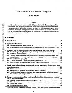
where wsri is the relative weight of each sum rule and Ai is the theoretical value of the corresponding sum rule, eqns. (6-9). We note that this definition introduces a new set of, in principle, arbitrary parameters, that is the relative weights of the sum rules. As explained below, these are determined by stability criteria, demanding that the contribution from Esr is similar to that of Eerr and that the final result is not sensitive to the specific values of these parameters. The basic idea of the genetic algorithms training, also known as natural selection training, works as follows. The training is divided in generations. For each generation the parameters of the network (weights and thresholds) are arranged to form a chain, called the ADN chain. This chain is replicated many times, creating a population of identical individuals. Later, random mutations are applied to each individual, where by mutation we mean a small change in one of the bits of his ADN chain. Then, the error function associated with each mutated individual is computed, which implies passing back the ADN bits to their original status of weights and thresholds and calculating the output of this new network. Only the best individuals are kept while discarding the rest, mimicking natural selection. This method provides a suitable technique to implement the effect of the chiral sum rules on our neural network training. Note that this technique leads to an important increase on the computing time, due to the fact that the chiral sum rules must be numerically evaluated many times each generation. The main advantage of genetic algorithms is that they allow neural networks to learn from error functions that may be as complicate as making impossible the use of backpropagation training. Furthermore, genetic algorithms can be proven to search efficiently the parameter space of solutions, exploring exponentially many more times reasonable outputs as compare to manifestly wrong ones. Genetic algorithms can also handle the training of very large neural networks. The parametrization obtained by means of the genetic algorithm training is represented in figure (2) where the output of the trained neural network, without and with the inclusion of the 11

3

3 Experimental ALEPH data Trained network output (with sum rules)

2.5

2.5

2

2

1.5

1.5 v_1(s)-a_1(s)

v_1(s)-a_1(s)

Experimental ALEPH data Trained net output (no chiral sum rules)

1

1

0.5

0.5

0

0

-0.5

-0.5

-1

-1 0

0.5

1

1.5

2 s [GeV^2]

2.5

3

3.5

4

0

0.5

1

1.5

2 s [GeV^2]

2.5

3

3.5

4

Figure 2: Output of the neural network trained over the experimental data, without chiral sum rules (left) and with chiral sum rules (right) incorporated in the training. Note that the effect of the chiral sum rules is that the network output reaches faster the asymptotic behavior of the spectral function.

chiral sum rules, is compared with the experimental data points together with the corresponding statistical errors. It is clear that the effect of the chiral sum rules on the trained neural network output is forcing it to reach faster the asymptotic behavior of the spectral function ρV −A (s). A common problem in the genetic algorithm learning techniques is getting stuck in a local minimum of the error function, far from the absolute minimum. In our training this difficulty has been bypassed by means of different simple modifications of the basic training procedure. First, within each generation large additional mutations are performed that allow the network configuration to escape from local minima. Secondly, as the training advances, the rate of the mutations decreases, allowing for way a better local learning. These modifications are instrumental to decrease the large duration of the training.

4.3

Results and validation

Once all the parameters of the training have been determined by stability criteria, an independent set of neural networks is trained on the spectral functions v1 (s) − a1 (s). The length of the training is fixed by studying the behavior of the error function E (0) , as defined in eq. (24) for the neural net fitted to the central experimental values, and asking that E (0) /Ndat stabilizes to a value close to one, which can be considered a good training. A number of checks is then performed in order to make sure that an unbiased representation of the probability density has been obtained. First, we have verified that the covariance of two data points computed from the Monte Carlo sample of nets is on average very close to the corresponding covariance matrix element of the data. Since correlations of the data are entirely due to systematic errors, this indicates that these errors are correctly reproduced. Statistical estimators are then constructed as in eq. (19) but now referred to the trained neural networks over the replicas, to explicitly verify that the training maintains all the experimental

12

ρV −A (s) Nrep 10 100 (net) r[ρV −A (s) ] 0.980 0.981 (net) r[σ ] -0.21 -0.20 (net) r[ρ ] 0.80 0.85 Table 2: Comparison between experimental and generated artificial data for the ρV −A (s) spectral function. information. The scatter correlation is now defined as (net)

r[ρV −A ] =



(exp) ρV −A

(net) ρV −A rep

D

E



(exp) − ρV −A dat dat (net) (exp) σs σs

D

E

D

(net) ρV −A rep

E



dat

,

(26)

and the corresponding values for the training of Nrep = 100 replicas are presented in table 2. It is seen that the central values and the correlations are well reproduced, whereas this is not the case for the diagonal errors. The average standard deviation for each data point computed from the Monte Carlo sample of nets is substantially smaller than the experimental error. This is due to the fact that the network is combining the information from different data points by capturing and underlying law, or that it is introducing a smoothing bias. This effect is enhanced by the inclusion of sum rules constraints. All networks have to fulfill these constraints which forces the fit to behave smoothly in a region where experimental data are very large. This should be understood as a success of the fitting procedure. (net)(k) The final set of neural networks ρi provides a representation of the probability measure in the space of structure functions, which can be used to estimate any functional average, defined as in. eq (17) using Nrep h i 1 X (net)(k) hF [ρV −A (s)]i = F ρV −A (s) . (27) Nrep i=1

In particular, the average and standard deviation of the nonperturbative condensates computed using the Monte Carlo sample will provide a determination of the central values and errors of these condensates.

4.4

Details of the genetic algorithm training

As explained above, in the second part of the training the chiral sum rules eqs. (6-9) are incorporated to the error functional, eq. (24). These sum rules act as constraints on the neural network output, that is, the main contribution to the error function (which determines the learning of the network) still comes from the diagonal errors, and the sum rules are only relevant in the region where the errors are larger. The relative weights of the chiral sum rules will be chosen according to a stability analysis. The effect of including sum rules in the learning procedure is responsible for enforcing the desire vanishing oof the ρV −A (s) spectral function, which is badly needed for a reliable extraction of the nonperturbative vacuum condensates. Obtaining maximum stability in our output is crucial for a proper parametrization of the spectral function. In the case of the relative weights of the chiral sum rules, we train the same 13

4

5 Contribution from errors Contribution from SR1

Contribution from errors Contribution from SR2

3.5

Partial contributions to the error function

Partial contributions to the error function

4 3

2.5

2

1.5

1

3

2

1 0.5

0 0.001

0.01

0.1 Relative weights of SR1 wsr_1

1

0 0.01

10

0.1

1 Relative weight of SR2 wsr_2

10

100

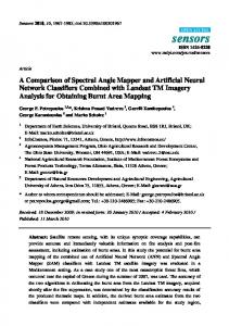
Figure 3: Dependence of the partial contributions to the error function on the relative weights of the SR1 (left) and SR2 (right) chiral sum rules. Note that as expected for normalized sum rules, the stability region for the relative weight is close to 1. network with different relative weights and search for the region where both contributions to the error function, the contribution from the errors and the contribution from the sum rules, are comparable. This is shown in figure (3). The observed behavior is not surprising: for large relative weights the contribution from the sum rule is small because the training forces its learning but, as a consequence, the contribution from the experimental data increases. This behavior can be observed explicitely if we plot the evolution of the sum rules, as calculated with the network output of the trained network, as a function of their relative weights. We observe in figure (4) that, as the relative weight increases, the network output better verifies the corresponding chiral sum rule. Genetic algorithms thus allow to implement additional constraints in the training of neural networks in a smooth and efficient way. Its main drawback is the increase of the training time, because it is a random rather than a deterministic learning technique. In figure (5) we represent an example of the training of one replica. It can be observed a sharp transition when the sum rules constraints are introduced, but later the training forces the error function to stabilize to a situation similar to the initial training epoch. This sudden jump of the error function can be understood as follows: when the sum rules constraints are introduced, the training tends to verify them, causing that the net output does not follow the experimental values. Nevertheless, as generations go on, the net output begins to recover the original situation, while maintaining the verification of the sum rules constraints. When the number of generations is large, the error function approaches a value close to one, as is needed to keep systematic errors under control. A key issue in this procedure is to guarantee stability of results with respect to the relative weights of the chiral sum rules. In our training normalized sum rules are used, that is, if Aj is the theoretical value of the j−th chiral sum rule, the corresponding contribution to the error function will be Z  wsrj

s0

0

2

dsfj (ρV −A (s)) − Aj

.

(Aj )2 ,

(28)

therefore we expect the relative weights in the stability region of order 1. The only exception is the second Weinberg sum rule, eq. (8) whose relative weight has to be determined demanding 14

0.04

0.1 Value of SR2 evaluated with NN output Exact value of SR2

Value of SR3 evaluated with NN output Exact values of SR3

0.035 0.08 0.03

values of SR3

Values of SR2

0.06 0.025

0.02

0.015

0.04

0.02

0.01 0 0.005 0.001

0.01

0.1 1 Relative weight of SR2

10

100

0.001

0.01

0.1 1 Relative weight of SR3 wsr_3

10

100

Figure 4: Dependence of the value of the SR2 (left) and SR3 (right) chiral sum rules on their relative weights. It is also clear how for a value of the relative weights close to 1 the chiral sum rules are satisfied. stability of the network training, and that turns out to be around wsr3 = 10−1 . Let us emphasize that the two Weinberg chiral sum rules are well verified by our neural network parametrization, and thus have been incorporated to the information contained on the experimental data. This fact will be crucial later because different extraction methods, differing in combinations of these chiral sum rules, can be shown to be equivalent in the asymptotic region s0 → ∞. In figure (6) the two Weinberg sum rules, eqs. (7,8) evaluated with the neural network parametrization of the spectral function ρV −A (s) are represented. Both chiral sum rules are well verified in the asymptotic region, beyond the range of available experimental data. This also will ensure the stability of the evaluation of the condensates with respect to the specific value of s0 chosen as long as it stays in the asymptotic region.

5

Determination of the nonperturbative condensates

Using the neural parametrization of spectral functions, we can compute for each trained replica any given sum rule. Because the neural parametrization retains all the experimental information (it even allows for a determination of errors and correlations), we can view values coming from the neural networks as direct experimental determinations of convolutions of the spectral function ρV −A (s). The value of the condensates hO6 i , hO8 i and higher dimensional condensates is then extracted from the value of an appropriate sum rule, eq. (12). The method we will follow is the evaluation of the vacuum condensates as a function of the upper limit of integration for each replica and compute the mean and standard deviation. As has been explained before, it is crucial to represent the value of the different sum rules as a function of the upper limit of integration, to check both its convergence and its stability. Our method works as follows. First, we train a neural network on each replica. On a first training epoch we do not use the sum rules, so that the training can arrive to the best possible minimum. This is important when training neural networks because when further constraints to the training are added, as in our case the chiral sum rules, the goodness of the fit will be better if we start from a deep local minimum. On a second training epoch, we add to 15

2.2 Total contribution Contribution from errors

Contributions to the error function

2

1.8

1.6

1.4

1.2

1

0.8

0.6 0

50000

100000

150000

200000 250000 300000 Number of generations

350000

400000

450000

500000

Figure 5: Dependence of the different contributions to the error function on the length of the training. Note the sudden jump when the sum rules are incorporated to the training, and how the network later return to a configuration similar to the initial one. the fitness the contribution from the sum rules, where the relative weights are chosen so that the sum rules never represent more than the contribution from the experimental errors to the total fitness. Then, sum rules act as a smooth constraint on the network training, being more relevant in the regions with larger errors and thus enforcing the asymptotic vanishing of the spectral function. This technique prevents the contribution of the chiral sum rules to become so strong that overcome the experimental data with the corresponding errors.

5.1

Central values

The first criterion to judge the reliability of a QCD sum rule is its independence, at large values of s from the value of the upper integration limit, that its, its saturation. We then need to explore the values for the final condensates which are stable against the limit of integration of the sum rule. This stability criterium is completed with demanding independence of the results on the specific polynomial entering the sum rule. Further criteria are stability with respect to the precise artificial endpoints added to the data and with respect to the relative weights in the error function used to train the neural networks. Stable results are obtained for the dimension six condensate hO6 i whereas higher condensates e. g. hO8 i are less stable. Fig. 1 shows the outcome for hO6 i and hO8 i including the propagation of statistical errors. It is clearly seen that convergence in the limit of integration s0 is obtained due to the addition of sum rules and endpoints in the learning procedure. The central values for the condensates in the asymptotic limit come out to be: s → ∞: hO6 i = −4.2 10−3 GeV6 , hO8 i = −12.7 10−3 GeV8 . 16

(29)

0.02

0.012 SR2 Exact result

SR3 Exact result

0.018

0.01

0.016

0.008 Second Weinberg chiral sum rule

First Weinberg chiral sum rule

0.014 0.012 0.01 0.008 0.006 0.004

0.006 0.004 0.002 0 -0.002 -0.004

0.002

-0.006

0 -0.002

-0.008 0

0.5

1

1.5

2 s_0 [GeV^2]

2.5

3

3.5

4

0

0.5

1

1.5

2 s_0 [GeV^2]

2.5

3

3.5

4

Figure 6: Weinberg chiral sum rules, SR2 (left) and SR3 (right), evaluated on the neural network parametrization of ρV −A (s) The value of the hO6 i is a cross check of the validity of our treatment: not only there are strong theoretical arguments that support the fact that hO6 i is negative [33], [35] but also all previous determinations with different techniques yield negative results, being the majority of them compatible with ours within errors. We note that our evaluation of the condensates is compatible with some of our previous evaluations and has a similar error. This is though misleading as the error quoted here is only statistical and a discussion on systematic errors is needed (and done below). We can also obtain values for the higher dimensional nonperturbative condensates: hO10 i = 7.8 10−2 GeV10 , hO12 i = −2.6 10−1 GeV12 .

(30)

Although stability deteriorates as compared to the case of the lower dimensional condensates, these central values for the condensates are alternated in sign.

5.2

Discussion of errors

The discussion of the various sources of errors is crucial to our treatment. We enumerate and discuss then in turn: 1. Statistical error propagation from the experimental covariance matrix. This is the best understood and treated error source in our analysis. As explained above, the neural network parametrization defines an unbiased probability measure in the space of spectral functions that provides a nonlinear error propagation. This source of error is kept under control by using the averages over Monte Carlo replica. The band for central values of the condensates allowed by this error propagation can be visualized in fig. (7). Numerically, the contribution to the experimental error (statistics and correlations) to the central values is hO6 i = (−4.2 ± 1.1) 10−3 GeV6 , 17

0.02

0.07 Dimension 6 condensate

Dimension 8 condensate 0.06

0.01

Dimension 8 condensate [GeV^8]

Dimension 6 condensate [GeV^6]

0.05

0

-0.01

-0.02

0.04 0.03 0.02 0.01 0 -0.01

-0.03 -0.02 -0.04

-0.03 0

0.5

1

1.5

2 s_0 [GeV^2]

2.5

3

3.5

4

0

0.5

1

1.5

2 s_0 [GeV^2]

2.5

3

3.5

4

Figure 7: Condensates hO6 i and hO8 i as a function of s0 . The error bands only include the propagation of experimental uncertainties.

hO8 i = (−12.7 ± 6.4) 10−3 GeV8 , hO10 i = (7.8 ± 2.4) 10−2 GeV10 , hO12 i = (−2.6 ± 0.8) 10−1 GeV12 .

(31)

Note that the sign obtained for each condensate remains unaltered within error. 2. Choice of the polynomial in the finite energy sum rule. In principle, there are potentially important systematic uncertainities coming from the method of extraction of the condensates. These are much more difficult to assess, as noted when looking through the extense available literature. The extraction of hO6 i turns out to be clean and its errors are essentially of statistical nature. The uncertainty increases with the dimension of the condensate. Let us elaborate further these statements. Consider the following convolutions Z6a ≡

Z

s0 0

ds

1 2 s ρV −A (s) 2π

(32)

1 s 2 1− ρV −A (s) − fπ2 s20 (33) 2π s0 0 The second equation is only equivalent to the first if, for some s0 , both Weinberg sum rules are satisfied. Although experimental data on tau decays do not exactly saturate these sum rules, the neural network parametrization trained to obey all the sum rules showed that Weinberg sum rules can indeed be well verified in the asymptotic region. We should then expect that Z6a and Z6b ≡ s20

Z

Z6b ≡

s0

Z

0

ds

s0

ds





 1  2 s − 2ss0 ρV −A (s) 2π

(34)

yields similar results for hO6 i within errors, as can be seen in fig. (8). The same applies to the dimension 8 condensate hO8 i, where we now define the following finite energy sum rules: Z s0 1 Z8a ≡ − ds s3 ρV −A (s) , (35) 2π 0 18

0.015

0.25 Z_6a(s_0) Z_6b(s_0)

Z_8a(s_0) Z_8b(s_0) Z_8c(s_0)

0.01 0.2 0.005 0.15 Dimension 8 condensate

Dimension 6 condensate

0 -0.005 -0.01 -0.015 -0.02

0.1

0.05

0

-0.025 -0.05 -0.03 -0.035

-0.1 0

0.5

1

1.5

2 s_0 [GeV^2]

2.5

3

3.5

4

0

0.5

1

1.5

2 s_0 [GeV^2]

2.5

3

3.5

4

Figure 8: Extraction of hO6 i and hO8 i with different polynomials  1  3 (36) s − ss20 ρV −A (s) , 2π 0 Z s0  1  3 Z8c ≡ − ds s + 3s20 s ρV −A (s) . (37) 2π 0 We conclude that the neural network parametrization of spectral functions properly trained to accomodate for all sum rules provides estimates for condensates which are independent of the choice of a specific finite energy sum rule.

Z8b ≡ −

Z

s0

ds

3. Dependence on the endpoints. Our fit implements the asymptotic constraint that ρV −A (s → ∞) = 0 by adding artificial endpoints. It is then necessary to verify the degree of sensitivity of our ouput to the precise location of these endpoints. As shown if Fig. (9), the sign of the dimension six and eight condensates remains unaltered when endpoints range between 3.5 and 4 GeV2 . We also observe relatively large, although compatible within errors, fluctuations of the central values. This effect may be related to the presence of small wiggles in the spectral function ρV −A (s) for large s. The contribution of this source of uncertainty to hO8 i turns to dominate over statistical uncertainties and can be estimated to be − 2.5 10−2 ≤ hO8 i ≤ −5 10−3

(38)

while for hO6 i is comparable to the uncertainty due to the statistical errors of the experimental data, that is, − 6 10−3 ≤ hO6 i ≤ −2 10−3 . (39) 4. Chiral sum rules. This turns out to be the main source of systematic errors for the dimension 6 condensate. Chiral sum rules can be forced to be fulfilled by adequate training to any desired degree of precision. This, though, introduces a large increase in the total error function, eq. (25), coming from the experimental error piece. It is then necessary to make an appropriate choice of relative weights between the error associated to experimental data and the error associated to the fulfillment of chiral sum rules. 19

0 Dimension 6 condensate

Dimension 8 condensate

-0.001

-0.005

-0.002 Dimension 8 condensate

Dimension 6 condensate

-0.01 -0.003

-0.004

-0.005

-0.015

-0.02

-0.025 -0.006

-0.03

-0.007

-0.008

-0.035 3

3.2

3.4

3.6

3.8 4 s Endpoint [GeV^2]

4.2

4.4

4.6

3

3.2

3.4

3.6

3.8 4 s Endpoint [GeV^2]

4.2

4.4

4.6

Figure 9: Value of the condensates hO6 i (left) and hO8 i (right) as a function of the position s of the first artificial endpoint. Note that their sign remains unchanged and the presence of a stability region near s = 3.5 GeV2 We may advocate that the most appropiate relative weights for the normalized chiral sum rules are O(1). This is due to the fact that the total error function jumps above 1 when too large relative weights are considered, as seen in figs. (3, 4). We have thus performed a multi-dimensional stability analysis searching for the relative weights that produce a minimum sensitive final result, supplemented with the condition that in any case the contribution from the experimental errors to the error function can be greater than 1. The most suitable relative weights for the chiral sum rules turn out to be wsr1 = 1.0 wsr2 = 5 102

wsr3 = 0.3 wsr4 = 1 102 .

(40)

This stability analysis shows that the sign of the central values of the condensates is not very sensitive to the relative weights for the chiral sum rules. The estimation of the error associated with this uncertainty leads to the following range of values for the lowest dimensional condensate − 2 10−3 ≤ hO6 i ≤ −6 10−3 GeV6 .

(41)

For hO8 i the statistical errors and the systematic error due to the position of the artificial endpoints turn out to dominate over this source of uncertainty. Similar estimates for the condensates of higher dimensions turn out not to be reliable, and therefore we present only the central values obtained in this analysis together with the statistical errors.

5.3

Analysis of the s0 = 1.5 GeV2 duality point

Some values of previous extraction of the condensates [27] are based on the existence of a duality point around s0 ∼ 1.5 GeV2 . Our neural network parametrization is such that the second Weinberg sum rules is indeed verified around this point. Consequently, the values of the condensates computed by truncating different finite energy sum rules at this point do agree, as can be seen in fig. (6). Nevertheless, as shown in fig. (8), the value of the condensates at this 20

duality point is different than the asymptotic one. Both results share the same sign but not the same absolute magnitude for hO6 i, and with the opposite sign for hO8 i (which is precisely the results that the authors in Ref. [27] obtain). These extractions using the first duality point can be justified by some resonance models of the hadronic spectrum [28], inspired in the large−NC limit of QCD with the additinal assumption of the validity of the Minimal Hadronic Approximation (MHA), in which the spectral functions are saturated by the pion pole, the first axial vector and the first rhoo vector resonances. Experimentally, it is observed that at different duality points, even as low as 1.5 GeV2 , there is a local quark-hadron duality, meaning that the OPE at the quark- gluon level and that evaluated with the entire resonance hadronic spectrum coincide. Whether this apparent duality point at s0 = 1.5 GeV2 is an accident only due to the fullfillment of the second Weinberg sum rule, or it is really a consequence of the full QCD hadronic spectrum remains to be understood. What it is clear from our analysis is that the condensates evaluated at this first duality point are different to those obtained in the asymptotic regime s0 → ∞, where the validity of the OPE is less questioned.

5.4

Spectral functions and the electroweak penguin Q7

As a byproduct of our analysis additional sum rules of the spectral function ρV −A which are relevant to phenomenology can be estimated. As an example3 , the sum rule ALR (µ2 ) ≡

Z

0

s0

s ds s2 ln µ2

!

1 ρV −A (s) , 2π 2

(42)

will be considered, where µ2 is a arbitrary factorization scale that cancels in the computation of physical observables. In this analysis the value µ2 = 2 GeV2 will be used. Eq. (42) is relevant to the evaluation of Im GE , where GE is one of the couplings of the low energy chiral Lagrangian describing |∆S| = 1 transitions [26]. The importance of a precise determination of this coupling relies on the fact that Im GE is one of the most important contributions to ǫ′ in the Standard Model. In turn, its value is dominated by the electroweak penguin contributions Q7 and Q8 , which explains why the data on spectral functions from hadronic tau decays is important in its determination. Following the same steps that lead to the determination of the vacuum condensates, the same procedure for the sum rule eq. (42) is repeated. The result that is obtained in the asymptotic limit s0 → ∞ is ALR = (6.9 ± 1.6) 10−3 GeV6 ,

(43)

as can be seen in figure (10). It should be noted that the present determination is in good agreement with that obtained in the original work4 [26]. The quoted error only refers to the propagation of experimental uncertainties. 3

In this section the work of Ref. [26] is followed, the reader is directed to this reference for definitions and notation 4 Note however that a different normalization for the spectral correator is used.

21

A_LR(s) 0.01

A_LR(s) [GeV^6]

0.005

0

-0.005

-0.01

-0.015

-0.02 0

0.5

1

1.5

2 s [GeV^2]

2.5

3

3.5

4

Figure 10: Evaluation of eq. (42) for diferent values of s0 . The error bands include the propagation of experimental uncertainties.

5.5

Results and comparison with other determinations

Our determination of the nonperturbative condensates including the statistical error coming from the experimental errors and correlations was given in eq. (31). However, the error which dominates the determination of hO6 i comes from the relative weights of the chiral sum rules to be obeyed. We have performed a stability analysis on these relative weights that produces a final result: hO6 i = (−4.0 ± 2.0) 10−3 GeV6 . (44) As explained above, for the dimension 8 condensate, the systematic error associated with the endpoint position is comparable to the statistical uncertainty, that combine to yield a value 

hO8 i = −12

+ 7 − 11



10−3 GeV8 .

(45)

For higher dimensional condensates it is much difficult to estimate the different sources of systematic uncertainties. We, then, quote the central values we obtained and their statistical error: hO10 i = (7.8 ± 2.4) 10−2 GeV10 , hO12 i = (−2.6 ± 0.8) 10−1 GeV12 .

(46)

A similar analysis has been performed with the OPAL data, yielding equivalent results but with larger errors, due to the larger statistical uncertainties as compared to the ALEPH experimental data. The values of the QCD nonperturbative condensates have been previously extracted from the ALEPH and OPAL data, with different techniques and different results, as summarized in table 3. Note that our results agree, at least on the sign, with that of Refs. [26], [29], [30]. This is also true for the higher dimensional condensates of Ref. [22], where the authors obtain: hO10 i = (4.8 ± 1.0) 10−2 GeV10 , 22

Reference Ref. [23] Ref. [24] Ref. [26] Ref. [27] Ref. [29] Ref. [30] This work

hO6 i × 103 GeV6 −6.4 ± 1.6 −6.8 ± 2.1 −3.2 ± 2.0 −9.5 ± 3 −4.45 ± 0.7 −4 ± 1 −4 ± 2

hO8 i × 103 GeV8 8.7 ± 2.4 7±4 −12.4 ± 9.0 16.2 ± 5 −6.2 ± 3.2 −1.2 ± 6 7 −12 −+ 11

Table 3: Previous extractions of the condensates ordered chronologically. Appropiate rescalings have been performed to allow the comparison of different extractions. hO12 i = (−1.6 ± 0.26) 10−1 GeV12 .

(47)

in agreement with eq. (31) , although the errors in our determination are somewhat larger. There are some differences between these previous determinations and the present one, eq. (46). The first one is that we do not make any assumption on the values of the higher dimensional nonperturbative condensates. In many analysis the effect of hOD i for D ≥ 10 is simply neglected to get closed expressions for the condensates. In our analysis, though, we do not need to make this hypothesis. Neither we need to assume that the chiral sum rules are verified, because the chiral sum rules enter as constraints in the genetic algorithm training (see fig. (6)). This is relevant because previous analysis showed that the chiral sum rules are not verified for s0 = Mτ2 , except the DMO sum rule, implying that one must be extremely careful when dealing with them. A second main difference is the absence of theoretical bias introduced in other analysis with a choice of a given finite energy sum rules. Moreover, the smooth interpolating capability of the neural network lets the integration range to be taken up to arbitrarily high energies.

6

Conclusions

We have presented a determination of the nonperturbative vacuum condensates hO6 i and hO8 i from the spectral functions from hadronic tau decays aimed at minimizing the sources of theoretical bias which might be cause of concern in existing determinations of these condensates from spectral functions. This determination is based on a bias-free neural network parametrization of the v1 (s) − a1 (s) spectral function, inferred from the data, which retains all the information on experimental errors and correlations, and supplemented with the additional theoretical input of the chiral sum rules. Our final results give negative central values for the dimension 6 and 8 condensates. These results take into account the propagation of statistical errors and their correlations. Morevover, the main source of systematic error in our procedure is identified as the choice of relative weights assigned to chiral sum rules in the fitness function used to train the neural networks. In the case of the dimension 6 condensate a stability analysis can be performed. Higher dimension condensates carry larger errors, although the sign of the condensates seem to remain unaltered. 23

The sign of the dimension eight condensate hO8 i deserves further comments. Our central value is negative within statistical errors but is sensitive to the position of artificial endpoints added to enforce the vanishing of the spectral function for large values of s. This produces a systematic bias as possible wiggles of the spectral function around the asymptotic zero value are suppreseed. Those wiggles may indeed produce a change of sign of hO8 i. This is not the case in our approach as the smoothness of the neural network tends to avoid such wiggles, which might lead to a systematic error. Although our results seem to point in the same direction of other recent previous extractions of hO8 i we consider the issue of the sign of the vacuum condensate hO8 i to remain open. Another result of this work is the implementation of a technique based on genetic algorithm neural network training, which extends the capabilities of neural network data analysis allowing to incorporate non-local constraints like convolutions in the training. This technique extends previous efforts [3] oriented to the improvement of high energy physics data analysis, specially for the strong interaction sector.

Acknowledgments It is a pleasure to thank S. Peris and E. de Rafael for suggesting the application of Ref. [1] to this problem and for fruitful discussions, and J. Prades and A. Pich for useful comments and suggestions. We would also like to thank A. Hoecker and W. Mader for their help with the experimental data of the ALEPH and OPAL collaborations respectively. This work was supported by the projects MCYT FPA2001-3598, GC2001SGR-00065 and by the Spanish grant AP2002-2415.

24

A

Neural network techniques

In this section a brief review of the neural network training algorithms that have been used in the this analysis is presented. Two different learning algorithms have been used for the neural network training: in a first epoch the only contribution to the error function comes from the statistical experimental errors, and the used learning algorithm is known as backpropagation. Then, in a second training epoch, the contribution from the chiral sum rules is added to the error function. As long as convolutions over the neural network output are non local constraints, the previous technique is no longer useful and another learning algorithm is needed, which is called genetic algorithms training. Now each of this techniques will be introduced, directing the interested reader to the standard reviews and textbooks [32] on neural networks and applications. Learning by backpropagation allows to train multilayer neural networks and has proved to be an excellent tool in classification, interpolation and prediction tasks. It is a standard technique that has been recently applied to data analysis in high energy physics, see Ref. [3]. The starting point is a set of input-output patters, (xµ , z) ∈ Rn × Rm , µ = 1, . . . , p ,

(48)

that network must learn. In our case, each input-output pattern consists of a single data point, the input being the energy s and the output the spectral function ρV −A (s). The basis of the network learning is the error function, also known as fitness functional. The error function is defined as the difference between the actual and the desired output of the net, measured over the training set, and weighted with the experimental errors. It is given by E=

N dat X i=1



(exp)

ρi

 (net) 2

− ρi

(exp)2

σi

.

(49)

Applying the gradient descent minimization procedure, that is, looking for the direction of steepest descent of the error function, the appropriate changes in the network parameters such that the error function decreases can be determined. The error is introduced in the units of the last layer by (L),µ (L)µ ∆i = g ′(hi ) [oi (~xµ ) − ziµ ] , (50) and then backpropagated to the rest of the network (l−1),µ ∆j

=g

′

nl (l−1)µ X (l),µ (l) ∆i ωij (hj ) i=1

,

(51)

and the last step consistes on the update of the weights and thresholds of the net (l) δωij

= −η

p X

(l)µ (l−1)µ

∆i ξj

(l)

+ αδωij (last) ,

(52)

µ=1 (l) δθi

= −η

p X

(l)µ

∆i

(l)

+ αδθi (last) ,

(53)

µ=1

where η is the learning rate parameter which controls the velocity of the training and the term with α is called a momentum term, which improves the algorithm so that the training does not 25

get stuck in a local minimum. The main advantage of this method is that it is deterministic and it has been used repeatedly in different situations, always successfully. As stated above, the second of the neural networks techniques that are used in our analysis is called genetic algorithm learning, also known as natural selection learning. As long as the chiral sum rules are convolutions of the network output, that is are non local functions on the error function, meaning that they depend not on a single network output but on the global output, the usual backpropagation training techniques are not useful in this second epoch of our training. Now the error functional has the form of eq. (49) but with additional convolutions of the neural network output E=

N dat X i=1



(exp)

ρi

 (net) 2

− ρi

(exp)2

σi

+

NX conv

wi

i=1

Z

s0



(net)

dsfi ρ

0



(s) − Ai



,

(54)

where Ai is the theoretical value of the i−th sum rule and wi is the relative weight of this sum rule. In this case genetic algorithms are used, a training method inspired in the evolutionary theories in biology. In this method, the network parameters are transformed into bits in an ADN chain. These chains are replicated, and then some bits are mutated with a certain probability, and only those chains with the smallest contribution to the error functional survive. By analogy, this method is also known as natural selection learning. A simple scheme of the recursive process can be seen as follows: the starting piont is the set of parameters that define the neural network, (1)

(2)

(1)

(2)

ω11 , ω11 , . . . , θ1 , θ1 , . . . ⇓ Creation of ADN chain ⇓ ADN1 =





(1) (2) (1) (2) ω11 , ω11 , . . . , θ1 , θ1 , . . .

⇓

Replication of ADN chains ⇓ 

(1)

(2)

(1)

(2)





(1)

(2)

(1)

(2)



ADN1 = ω11 , ω11 , . . . , θ1 , θ1 , . . . , ADN2 = ω11 , ω11 , . . . , θ1 , θ1 , . . . . . . ⇓

Random mutation of bits in the ADN chains ⇓ 

(1)

(2)

(1)

(2)





(1)

(1)

(1)

(1)



ADN1 = ω11 , ω11 , . . . , θ1 , θ1 , . . . , ADN2 = ω11 + δ2 ω11 , . . . , θ1 + δ2 θ1 , . . . . . . ⇓

Selection of best ADN chain

26

⇓ (1)



(1)

(1)

(1)



ADNj = ω11 + δj ω11 , . . . , θ1 + δj θ1 , . . . ⇓

New weights and thresholds and decrease of fitness ⇓ (1) ω11

+

(1) (1) δj ω11 , . . . , θ1

(1)

+ δj θ1 , . . .

This is a very simple genetic algorithm, more modifications could be added to improve its efficiency like crossing between individuals (characterized by an ADN chain), but our analysis showed that this was not necessary. Its main drawbacks are that it is random rather than deterministic as is the backpropagation algorithm, and that requires to carefully adjust many parameters (rate of mutations, size of the population). These parameters have been adjusted following two requirements: efficiency of the learning and stability of the result. Learning by genetic algorithms allows therefore to impose the theoretical constraints from the chiral sum rules in a natural way. Finally, we would like to comment on a new learning algorithm that implements the main advantages of the two methods, that is, it is deterministic and therefore the simulation time is smaller, but at the same time it supports non local contributions to the error function. During the realization of this work, a novel technique was developed that allowed to use the backpropagation learning algorithms in the case of eq. (54), when the error functional contains convolutions. This allowed to check that the results obtained with the genetic algorithm approach were correct. In brief, this technique consists in noticing that an integral can be determined up a any desired accuracy by a finite sum of local contributions, when in this context local means that only depends on one network output. In fact, this is what any numerical integration method does, so it is clear that training algorithms for backpropagation learning can be implemented. The result is that for a discretization of the integral of the form Z

dxf (x) =

n X

cj fj ,

(55)

j=1

where the coefficients depend on the method, applying the usual backpropagation condition (variation of weights and thresholds in the direction of steepest descent of the error function) to the convolution term one finds that corresponding equations are the backpropagation equations but with eq. (50) replaced by (L)k

∆1



= 2

ns X

j=1



cj fb − A ca

df ′ (L) zg (h1,k ) , dok

(56)

where for simplicity we have only considered one sum rule and z is a normalization factor present due to the fact that the inputs and outputs of the neural network are normalized, so that the activation function of the neurons are always within the sensibility range of the activation function. In eq. (56) ok means the output of the network when the input xk is introduced, f (o(x)) is the convolution that we want the network to learn and A is its theoretical value. In this equation each term should be understood as a new pattern for the neural network 27

training. From here the usual backpropagation techniques apply as usual. This novel technique was implemented in the present analysis but it did not improve neither the quality nor the speed of the training, so the genetic algorithms technique was mantained for the training with convolutions. This technique, that is called backpropagation for convolutions, has many applications, and will be the subject of future work.

References [1] S. Forte, J.I. Latorre, L. Magnea, A. Piccione, Nucl. Phys. B643 (2002) 477, hep-ph/0205286. [2] A. Piccione, Aspects of QCD perturbative evolution, Ph.D. thesis, hep-ph/0207204. [3] S. Forte, L. Garrido, J.I. Latorre and A. Piccione, JHEP 0205 (2002) 062, hep-ph/0204232. [4] Y.S. Tsai, Phys. Rev. D4 (1971) 2821. [5] A. Hoecker, Ph.D. Thesis, Report LAL 97-18, Orsay, France (1997). [6] A.J. Buras, Weak hamiltonian, CP violation and rare decays, hep-ph/9806471.

TASI lectures,

[7] R. Barate et al., the ALEPH Collaboration, Eur. Phys. J. C4,409(1998). [8] R. Barate et al., the ALEPH Collaboration, Z. Phys. C71 (1997) 15. [9] K. Ackerstaff et al., The OPAL collaboration, Eur. Phys. J. C7,571(1999). [10] E. Braaten, S. Narison and A. Pich, Nucl. Phys. B373 (1992) 581. [11] E.G. Floratos, S. Narison, E. de Rafael, Nucl. Phys.B155 (1979) 115-149. [12] ’Review of particle physics’,Phys. Rev. D66, 1 (2002). [13] M. Shifman, A.I. Vainshtein, V.I. Zakharov, Nucl. Phys. B147 (1979) 385. [14] E. de Rafael, ’An introduction to sum rules in QCD’, Les Houches 1997 lectures, hep-ph/9802448. [15] S. Narison , ’QCD Spectral Sum Rules’, World Scientific Lecture Notes in Physics Vol. 26, World Scientific, Singapore 1989. [16] J. Gasser and H. Leutwyler, Annals Phys. 158 142 (1984). [17] E.C. Poggio, H.R. Quinn and S. Weinberg, Phys. Rev. D13 (1976) 1958. [18] T. Das, V.S. Mathur and S. Okubo, Phys. Rev. Lett. 19 (1967) 895. [19] S. Weinberg, Phys. Rev. Lett. 18 (1967) 507.

28

[20] T. Das, G.S. Guralnik, V.S. Mathur, F.E. Low and J.E. Young, Phys. Rev. Lett. 18 (1967) 759. [21] F. Le Diberder and A. Pich, Phys. Lett. B289 (1992) 165. [22] V. Cirigliano, J.F. Donoghue, E. Golowich and K. Maltmann, Phys. Lett. B522 (2001) 245. [23] M. Davier, L. Girlanda, A. Hocker and J. Stern, Phys. Rev. D58 (1998) 096014. [24] B.L. Ioffe and K.N. Zyablyuk, Nucl.Phys. A687 (2001) 437, hep-ph/0010089. [25] M. Shifman, hep-ph/0009131. [26] J. Bijnens, E. Gamiz and J. Prades, JHEP 0110 009 (2001), hep-ph/0108240. [27] M. Knecht, S. Peris and E. de Rafael, Phys. Lett. B508 (2001) 117. [28] M. Golterman, S. Peris, B. Phily and E. de Rafael, JHEP 0201 024 (2002), hep-ph 0112042. [29] V. Cirigliano, E Golowich and K Maltman, hep-ph/0305118.

Phys.Rev. D68 (2003) 054013,

[30] C.A. Dom´inguez and K. Schiler, hep-ph/0309285. [31] Sergio Gomez Jimenez, Ph.D. Thesis, Universitat de Barcelona [32] C. Peterson and T. R¨ognvaldsson, Lectures at the 1991 CERN School of Computing, preprint LU-TP-91-23; B. M¨ uller, J. Reinhardt and M. T. Strickland, Neural Networks: an introduction (Berlin, 1995); G. Stimpfl-Abele and L. Garrido, Comput. Phys. Commun. 64 (1991) 46. [33] E. Witten, Phys. Rev. Lett. 51 (1983) 2351. [34] M. Knecht, E. de Rafael, Phys. Lett. B424 (1998) 335, hep-ph/9712457 [35] J. Comellas, J.I. Latorre and J Taron, Phys. Lett. B360 (1995) 109, hep-ph/9507258.

29