Outline. ♢ Brains. ♢ Neural networks. ♢ Perceptrons. ♢ Multilayer perceptrons. ♢
Applications of neural networks. Chapter 20, Section 5. 2 ...
Neural networks
Chapter 20, Section 5
Chapter 20, Section 5
1
Outline ♦ Brains ♦ Neural networks ♦ Perceptrons ♦ Multilayer perceptrons ♦ Applications of neural networks
Chapter 20, Section 5
2
Brains 1011 neurons of > 20 types, 1014 synapses, 1ms–10ms cycle time Signals are noisy “spike trains” of electrical potential
Axonal arborization Axon from another cell Synapse Dendrite
Axon
Nucleus Synapses
Cell body or Soma
Chapter 20, Section 5
3
McCulloch–Pitts “unit” Output is a “squashed” linear function of the inputs: ai ← g(ini) = g Σj Wj,iaj �
a0 = −1
aj
�
Bias Weight
ai = g(ini)
W0,i Wj,i
Input Links
ini
g
Σ
Input Activation Function Function
ai
Output
Output Links
A gross oversimplification of real neurons, but its purpose is to develop understanding of what networks of simple units can do
Chapter 20, Section 5
4
Activation functions g(ini)
g(ini)
+1
+1
ini
ini
(a)
(b)
(a) is a step function or threshold function (b) is a sigmoid function 1/(1 + e−x) Changing the bias weight W0,i moves the threshold location
Chapter 20, Section 5
5
Implementing logical functions W0 = 1.5
W0 = 0.5
W1 = 1
W0 = – 0.5
W1 = 1
W2 = 1
W1 = –1
W2 = 1 AND
OR
NOT
McCulloch and Pitts: every Boolean function can be implemented
Chapter 20, Section 5
6
Network structures Feed-forward networks: – single-layer perceptrons – multi-layer perceptrons Feed-forward networks implement functions, have no internal state Recurrent networks: – Hopfield networks have symmetric weights (Wi,j = Wj,i) g(x) = sign(x), ai = ± 1; holographic associative memory – Boltzmann machines use stochastic activation functions, ≈ MCMC in Bayes nets – recurrent neural nets have directed cycles with delays ⇒ have internal state (like flip-flops), can oscillate etc.
Chapter 20, Section 5
7
Feed-forward example
1
W1,3
3
W1,4
W3,5 5
W2,3 2
W2,4
4
W4,5
Feed-forward network = a parameterized family of nonlinear functions: a5 = g(W3,5 · a3 + W4,5 · a4) = g(W3,5 · g(W1,3 · a1 + W2,3 · a2) + W4,5 · g(W1,4 · a1 + W2,4 · a2)) Adjusting weights changes the function: do learning this way! Chapter 20, Section 5
8
Single-layer perceptrons
Input Units
Wj,i
Output Units
Perceptron output 1 0.8 0.6 0.4 0.2 0 -4 -2 0 x1
2
4
-4
4 2 0 x2 -2
Output units all operate separately—no shared weights Adjusting weights moves the location, orientation, and steepness of cliff
Chapter 20, Section 5
9
Expressiveness of perceptrons Consider a perceptron with g = step function (Rosenblatt, 1957, 1960) Can represent AND, OR, NOT, majority, etc., but not XOR Represents a linear separator in input space:
Σj Wj xj > 0 or W · x > 0 x1
x1
x1
1
1
1
? 0 0
1 (a) x1 and x2
x2
0 0
1 (b) x1 or x2
x2
0 0
1
x2
(c) x1 xor x2
Minsky & Papert (1969) pricked the neural network balloon Chapter 20, Section 5
10
Perceptron learning Learn by adjusting weights to reduce error on training set The squared error for an example with input x and true output y is 1 1 2 E = Err ≡ (y − hW(x))2 , 2 2 Perform optimization search by gradient descent: � ∂Err ∂ � ∂E n = Err × = Err × y − g(Σj = 0Wj xj ) ∂Wj ∂Wj ∂Wj = −Err × g 0(in) × xj
Simple weight update rule: Wj ← Wj + α × Err × g 0(in) × xj E.g., +ve error ⇒ increase network output ⇒ increase weights on +ve inputs, decrease on -ve inputs Chapter 20, Section 5
11
Perceptron learning contd.
1 0.9 0.8 0.7 0.6 0.5
Perceptron Decision tree
0.4 0 10 20 30 40 50 60 70 80 90 100 Training set size - MAJORITY on 11 inputs
Proportion correct on test set
Proportion correct on test set
Perceptron learning rule converges to a consistent function for any linearly separable data set 1 0.9 0.8 0.7 0.6 0.5 0.4
Perceptron Decision tree 0 10 20 30 40 50 60 70 80 90 100 Training set size - RESTAURANT data
Perceptron learns majority function easily, DTL is hopeless DTL learns restaurant function easily, perceptron cannot represent it
Chapter 20, Section 5
12
Multilayer perceptrons Layers are usually fully connected; numbers of hidden units typically chosen by hand Output units
ai
Wj,i
Hidden units
aj
Wk,j
Input units
ak
Chapter 20, Section 5
13
Expressiveness of MLPs All continuous functions w/ 2 layers, all functions w/ 3 layers
hW(x1, x2) 1 0.8 0.6 0.4 0.2 0 -4 -2 x1
0
2
4
-4
4 2 0 x2 -2
hW(x1, x2) 1 0.8 0.6 0.4 0.2 0 -4 -2 x1
0
2
4
-4
4 2 0 x2 -2
Combine two opposite-facing threshold functions to make a ridge Combine two perpendicular ridges to make a bump Add bumps of various sizes and locations to fit any surface Proof requires exponentially many hidden units (cf DTL proof) Chapter 20, Section 5
14
Back-propagation learning Output layer: same as for single-layer perceptron, Wj,i ← Wj,i + α × aj × ∆i where ∆i = Err i × g 0(in i) Hidden layer: back-propagate the error from the output layer: ∆j = g 0(in j )
X
i
Wj,i∆i .
Update rule for weights in hidden layer: Wk,j ← Wk,j + α × ak × ∆j . (Most neuroscientists deny that back-propagation occurs in the brain)
Chapter 20, Section 5
15
Back-propagation derivation The squared error on a single example is defined as E=
1X (yi − ai)2 , 2 i
where the sum is over the nodes in the output layer. ∂ai ∂g(in i) ∂E = −(yi − ai) = −(yi − ai) ∂Wj,i ∂Wj,i ∂Wj,i ∂in ∂ X i = −(yi − ai)g 0(in i) = −(yi − ai)g 0(in i) Wj,iaj ∂Wj,i ∂Wj,i j = −(yi − ai)g 0(in i)aj = −aj ∆i
Chapter 20, Section 5
16
Back-propagation derivation contd. ∂ai ∂g(in i) ∂E X X = − (yi − ai) = − (yi − ai) i i ∂Wk,j ∂Wk,j ∂Wk,j ∂in ∂ X X i X = − (yi − ai)g 0(in i) = − ∆i Wj,iaj i i ∂Wk,j ∂Wk,j j ∂aj ∂g(in j ) X X = − ∆iWj,i = − ∆iWj,i i i ∂Wk,j ∂Wk,j ∂in j X = − ∆iWj,ig 0(in j ) i ∂Wk,j ∂ X X = − ∆iWj,ig 0(in j ) Wk,j ak i ∂Wk,j k X = − ∆iWj,ig 0(in j )ak = −ak ∆j i
Chapter 20, Section 5
17
Back-propagation learning contd. At each epoch, sum gradient updates for all examples and apply Training curve for 100 restaurant examples: finds exact fit Total error on training set
14 12 10 8 6 4 2 0 0
50
100 150 200 250 300 350 400 Number of epochs
Typical problems: slow convergence, local minima
Chapter 20, Section 5
18
Back-propagation learning contd.
Proportion correct on test set
Learning curve for MLP with 4 hidden units: 1 0.9 0.8 0.7 0.6
Decision tree Multilayer network
0.5 0.4 0
10 20 30 40 50 60 70 80 90 100 Training set size - RESTAURANT data
MLPs are quite good for complex pattern recognition tasks, but resulting hypotheses cannot be understood easily
Chapter 20, Section 5
19
Handwritten digit recognition
3-nearest-neighbor = 2.4% error 400–300–10 unit MLP = 1.6% error LeNet: 768–192–30–10 unit MLP = 0.9% error Current best (kernel machines, vision algorithms) ≈ 0.6% error
Chapter 20, Section 5
20
Summary Most brains have lots of neurons; each neuron ≈ linear–threshold unit (?) Perceptrons (one-layer networks) insufficiently expressive Multi-layer networks are sufficiently expressive; can be trained by gradient descent, i.e., error back-propagation Many applications: speech, driving, handwriting, fraud detection, etc. Engineering, cognitive modelling, and neural system modelling subfields have largely diverged
Chapter 20, Section 5
21