t each instant k+1, starting with k=d, ep 1. The neurones in the input layer receive the measured sequence x(k),...,x(k-d). Hence, in the first step the number of ...
Computational Modelling, Control & Automation M- Mohammadian (Ed.) IOS Press, 1999
Intelligence
for
63
Neural recurrent modelling for multi-steps time series prediction I.M. Galvan-Leon, E. Nogal-Quintana and J.M. Alonso-Weber Dep. of Computer Science. Universidad Carlos III, Av. de la Universidad 30, 28911 Leganes, Madrid, Spain
Abstract This paper is focused on the development of nonlinear neural models with the purpose of long-term or multistep time series prediction schemes. Multi-step prediction tries to achieve predictions several steps ahead into the future starting from information at time k. In the context of time series prediction, the most popular neural models are based on the traditional feedforward neural network. However, this kind of models may present some problems when a long-term prediction problem is formulated. In this paper, a neural model based on a partially recurrent neural network is proposed as an alternative. For the new model, a learning phase with the purpose of long-term prediction is imposed, which allows to obtain better predictions of time series in the future. The recurrent neural model has been applied to the logistic time series with the aim to predict the dynamic behaviour of the series in the future. Models based on feedforward neural networks have been also used and compared against the proposed model.
1. Introduction The ability to forecast the behaviour of a system hinges, generally, on the knowledge of the laws underlying a given phenomenon. When it is expressed as a solvable equation, one can predict the behaviour along the future once the initial condition is given. However, phenomenological models are often unknown or extremely time consuming. Nevertheless, it is also possible to predict the dynamic behaviour of the system along the future by extracting knowledge from the past. We are interested in time series processes which can be viewed as generalized nonlinear autoregressive models, also named NAR models. In this case, the time series behaviour can be captured by expressing the value x(k+l) as a function of the d previous values of the time series, x(k),...,x(k-d), that is: x(k + l) = F(x(k),...,x(k-d))
(1)
where k is the time variable and F is some function defining a very large and general class of time series. This function can be very complex and its explicit form is usually unknown. The standard prediction method involves approximating the function F in such way that the model given by eq.l allows to predict or find the sequence x(k+l),x(k+2),x(k+3),... starting from the observed sequence at the current time k, x(k),...,x(k-d). In many time series applications, one-step prediction schemes are used to predict the next sample of data based on previous samples. However, one-step prediction may not provide enough information, specially in situations where a broader knowledge of the time series behaviour can be very useful or in situations where it is desirable to anticipate the behaviour of the time series process. The present study deals with long-term or multi-step prediction, i.e. how to achieve predictions several steps ahead into the future, x(k+l),...,x(k+h), starting from information 1
64
l.M. Galvan-Leon et at. / Neural Recurrent Modelling
at time k. Hence, the goal is to approximate the function F such that the model given by eq. 1 can be used as a multi-step prediction scheme. The neural models most widely used in time series applications are built up using multilayer feedforward neural networks [1-3]. However, these models may not produce efficient predictions along the interval [k+l,k+h] because they have exclusively been trained with the purpose of one-step prediction. In this paper, a recurrent neural multi-step prediction model is presented, which is based on a partially recurrent neural network. The neural network has feedback connections from the output to the input layer and its parameters are determined with the purpose of longterm prediction. Therefore, this recurrent neural model is expected to provide better predictions than traditional feedforward neural models.
2. Multi-step prediction neural models In this section, the traditional neural models for the purpose of multi-step prediction are reviewed and their disadvantages are outlined. In the next one, the recurrent neural model is presented as an alternative to traditional models. 2.1. Traditional neural models The use of traditional neural models consists of approximating the function F appearing in eq. 1 by a multilayer feedforward neural network as follows: x(k + l) = F(x(k),...,x(k-d),W l ) (2) where Wi is the parameter set of the model, which is obtained using the backpropagation algorithm [4]. The update of the parameter set is based on the local difference between the measured and predicted values, i.e.: e(k + l) = —(x(k + l ) - x ( k + l)) 2 (3) 2 When the model given by eq. 2 has to predict the behaviour of time series in the future, i.e. along the interval [k+1, k+h], its structure has to be modified. The predictive network output must be fed back as an input for the next prediction and all the remaining input neuron values are shifted back one unit, i.e., x(k + l) = F(x(k),...,x(k-d),W,)
(4)
x(k + 2) = F(x(k +1), x(k),..., x(k - d + 1), W,)
(5)
x(k + h + 1) = F(x(k + h),...x(k + l),x(k),...,x(k - d + h), W,)
(6)
The main disadvantage of feedforward models in the context of multi-step prediction is that the parameter set has been obtained with the purpose of one-step prediction, i.e. to minimise the local errors given by eq. 3. During the training phase, the model captures the relation between the actual observations of the original time series, x(k),...,x(k-d) and the next sampling time, x(k+l). However, when the model is acting as multi-step prediction scheme (see eq. 4-6) a group of the input neurones receives the earlier approximated values, x(k + h),...x(k + l),x(k),...,x(k-d + h). This fact may produce a non desired behaviour of the model when a multi-step prediction problem is posed because errors occurred at some instant are propagated to future sampling times. Thus, the capability of traditional neural model to predict the future may decrease. 2
I.M.
Galvan-Leon
et
al.
/
Neural
Recurrent
Modelling
65
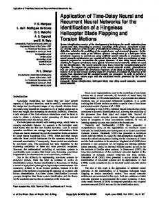
2. Recurrent neural model The recurrent neural model proposed in this paper is presented as an alternative to aditional neural models when the goal is to predict the future behaviour of time series, asically, the recurrent model consists of imposing a special learning phase with the purpose long-term prediction. The recurrent neural model is based on a partially recurrent neural network [5]. The network consists of adding feedback connections to a multilayer feedforward neural network om the output neurone to the input layer. The number of recurrent connections depends on e prediction horizon value. If the horizon is h, the input layer of the network is formed by a oup of h neurones that memorize previous network outputs; generally, these neurones are tiled context neurones. The remaining neurones in the input layer receive the original or easured time series data (see fig. 1). When the prediction horizon, h, is higher than the jmber of input neurones, d+1, all input neurones of the network are context neurones and > measured time series value is fed into the network.
Input layer Hidden layer Output layer Figure 1. Partially recurrent neural network
In the context of multi-step time series prediction, the training procedure of the partially current neural network is carried out as follows: t each instant k+1, starting with k=d, ep 1. The neurones in the input layer receive the measured sequence x(k),...,x(k-d). Hence, in the first step the number of context neurones is zero and the network output is given by: x(k + l) = F(x(k),...,x(k-d),W2) (7) ep 2. The number of context neurones is increased by one unit; this neurone memorizes the previously calculated output of the network, x(k +1). Thus, the prediction at instant k+2 is given by: x(k + 2) = F(x(k + l),x(k),...,x(k-d + l),W2) (8) ep 3. Step 2 is repeated until h context neurones are achieved. When the instant k+h+1 is reached, the output of the recurrent model is given by: x(k + h + l) = F(x(k + h),...x(k + l),x(k),...,x(k-d + h),W2) (9) ep 4. At this moment, the parameter set of the recurrent neural model, W2, is updated. In order to impose a training phase with the purpose of long-term prediction, the learning is based on the sum of the local errors along the prediction horizon, i.e. along the interval [k+1, k+h]. Hence, the parameter set W2 is updated following the negative gradient direction of the error function given by: 3
66
l.M. Galvan-Leon et al. / Neural Recurrent Modelling
1
h
2
i=i
e(k +1) = - • J ) (x(k + i +1) - x(k + i +1))2 (10) Since the internal structure of the partially recurrent network is like a feedforward neural network, the training can be realised using the traditional backpropagation algorithm, although other extensions of this algorithm should be feasible [6-7]. Step 5. At this point the time variable k is increased by one unit and the procedure returns to step 1. The procedure finalises when the instant k=N-h is reached, where N stands for the number of patterns. The structure of the recurrent model (eq. 7-9) is identical to the structure of the traditional neural model when it is used for prediction (eq. 4-6). However, there exists an important difference between them: the way to obtain the parameter sets of the models. As it was said before, the parameter set Wi is obtained training a multilayer feedforward network and remains fixed during the prediction phase. This means that the parameter set Wi is updated using the local error measured at each instant (eq. 3). When the recurrent neural model is used, the update of the parameters at each instant is based on the measured error along the prediction interval [k+1, k+h]. Thus, the set of parameters W2 has been determined to minimize the prediction error in the future. In consequence, the recurrent model is trained in such way that it acts as a multi-step prediction scheme as opposed to the traditional model given by eq. 2 which is trained to predict exclusively the next sampling time (one-step prediction scheme). Due to the recurrent structure of the proposed model, errors occurred at the same instant are propagated into the next sampling time as usual in the traditional neural models. However, in the recurrent neural model the propagated errors are reduced during the training phase because the learning is carried out using the predicted output at earlier time steps. Thus, the errors are corrected and better predictions in the future may be expected.
3. Experimental verification The simulations have been conducted and applied to the map of the form: x(k + l) = X x ( k ) ( l - x ( k ) ) (11) with X = 3.97 . This map describes a strongly chaotic time series which is called logistic time series. Two different structures of NAR models have been considered, named Model 1 and Model 2. From equation 11, it follows that the logistic map at instant k+1 depends on the value at instant k. Hence, the first NAR model has the following structure: Model 1: x(k +1) = F(x(k)) (12) As the ultimate goal in this paper is to predict the future, it is suitable to consider NAR models that own more information about the past behaviour of the time series. Thus, a second NAR model has been considered which is given by the following structure: Model 2: x(k + l) = F(x(k),x(k-l),x(k-2)) (13) Each model structure has been identified using both the feedforward neural network and the partially recurrent neural network. The capability of neural models to predict the future has been evaluated using the following error function: .
N-li
E = — Y(x(k + h)-x(k + h))2 2N S
(14) 4
67
I.M. Galvan-Leon et al. /Neural Recurrent Modelling
where h is the prediction horizon and N is the number of test patterns. In this work, four prediction horizons, h=l, h=2, h=3 and h=4, have been used to test the capability of neural models to predict the future. The prediction errors (eq. 14) for the first and the second structure of NAR models (eq. 12, 13) are presented in Table 1 and Table 2, respectively.
Model 1
Model 2
Prediction horizons h=l
Traditional Neural Model 0,00154
Recurrent Neural Model 0,00154
Prediction horizons h=l
Traditional Neural Model 0,00152
h=2
0,01006
0,00586
h=2
0,00904
0,00464
h=3
0,04667
0,01809
h=3
0,04807
0,00784
h=4
0,11900
0,09592
h=4
0,07827
0,01123
Table 1. Prediction Errors in Model 1
Recurrent Neural Model 0,00152
Table 2. Prediction Errors in Model2
In figure 2, figure 3 and figure 4 some of the predictions of the logistic time series provided by the traditional neural model and the recurrent neural model for the different structures of NAR model are shown.
0
10
2030405060
70 8 0 9 0 0 10 2 0 3 0 4 0 5 0 6 0 Figure 2. Model 1, Horizon=3 (a) Traditional neural model (b) Recurrent neural model
70
0
10
2030405060
70
8090
0
10
2030405060
70
8090
70 8 0 9 0 0 10 2 0 3 0 4 0 5 0 6 0 Figure 3. Model2, Horizon=3 (a) Traditional neural model (b) Recurrent neural model
70 8 0 9 0 0 10 2 0 3 0 4 0 5 0 6 0 Figure 4. Model2, Horizon=4 (a) Traditional neural model (b) Recurrent neural model
8090
5
f>8
I.M. Galvdn-Leon et al. / Neural Recurrent Modelling
4. Discussion and Conclusions From the experimental results we can conclude that the second structure of NAR model is more adequate to predict the future of the logistic time series because the model has more information about the behaviour of the time series through the extended number of input neurones. Both the traditional neural model and the recurrent neural model provide better approximations when this structure is used (see Table 1 and Table2). The Model 1 is able to predict the future when short prediction horizons are defined. However, when the prediction horizon is increased, the performance of this structure of model decreases (see Table 1). When the prediction horizon is fixed to four sampling times, both traditional and recurrent neural models do not provide appropriate predictions. This is due to the fact that these models do not own enough information about the time series. Hence, if the goal is multi-step prediction, the number of the inputs have an important significance on the quality of predictions. Assuming that the structure of NAR model has enough information through the input in order to predict the future, the immediate question that arises concerns the choice of the neural approach to be used. The results presented in the previous section show that models based on the partially recurrent neural network provide better approximations than models built up with multilayer feedforward neural networks (see Table 1 and Table2). The recurrent neural model has been trained with the purpose of multi-step prediction which seems to be a better approach. Furthermore, it is pointed out that the improvement of recurrent neural models over traditional ones is more significant when the prediction horizon is increased (see Table 2). For short prediction horizons (h=2), the approximations provided by the traditional neural models are adequate; although even in this cases the recurrent models obtain the smallest prediction errors. This superiority is more evident for long-term predictions (h=3, h=4). In consequence, for short prediction horizons the traditional models may be more suitable because they provide acceptable predictions and they are easier to build up. However, if the prediction horizon increases, the most convenient performance is provided by the recurrent neural model.
References [1] A.S. Weiggend, B.A. Huberman and D.E. Rumelhart: Predicting the future: A Connectionist Approach. Technical Report: PARC-SSL-90-20, April, 1990. [2] M. Cottrell, B. Girard, Y. Girard, M. Mangeas and C. Muller: Neural Modeling for Time Series: A Statistical Stepwise Method for Weight Elimination. IEEE Transations on Neural Networks, 6, N° 6, (1995) 1355-1363. [3] Hee-Yeal Yu and Sung-Yang Bang: An Improved Time Series Prediction by Applying the Layer-byLayer Learning Method to FIR Neural Networks. Neural Networks, 10, N° 9 (1997) 1717-1729. [4] D. Rumelhart, G. Hinton and R.J. Williams: Learning Internal Representations by Error Propagation, in Parallel Distributed Processing, MIT Press, Cambridge 1986. [5] I.M Galvan and J.M. Zaldivar: Application of recurrent neural networks in batch reactors. Part I. NARMA Modelling of the dynamic behaviour of the heat transfer fluid temperature. Chemical Engineering and Processing, 36 (1997) 505-518. [6] K. S. Narendra and K. Parthasarathy: Gradient methods for the optimization of dynamical systems containing neural networks, IEEE Trans, on Neural Networks, 2 (1991) 252-262. [7] D. Barrios, I.M. Galvan, P. Isasi and J. Rios: "NARMA recurrent neural modelling for controlling chemical batch reactors". Technical Report. UC3M-TR-CS-97-3. Department of Computer Science, Universidad Carlos III de Madrid, 1998.
6