Neuro-Fuzzy Dynamic Programming for Decision

51st Aerospace Sciences Meeting

Neuro-Fuzzy Dynamic Programming for Decision-Making and Resource Allocation of Wildland Fires

Journal:


Manuscript ID:

Draft

luMeetingID:

1965

Date Submitted by the Author: Contact Author:

n/a Hanlon, Nicholas

http://mc.manuscriptcentral.com/aiaa-masm13

Page 1 of 20


Neuro-Fuzzy Dynamic Programming for Decision-Making and Resource Allocation during Wildland Fires Nicholas Hanlon1, EDAptive Computing, Inc., Dayton, OH, 45458 Manish Kumar2, University of Toledo, Toledo, OH, 43606 and

Kelly Cohen3 University of Cincinnati, Cincinnati, OH, 45221 This paper proposes implementing fuzzy logic to improve upon the decision-making and resource allocation during a wildland fire. The problem is based on previous work of implementing neural dynamic programming in the theater-missile defense problem. The scenario was modified to the parameters of a wildland fire and extended to include multiple layers of defense. Three key areas were studied to evaluate the performance of the algorithm: sensitivity to engagement probability, uncertainty analysis, and scalability. The control methodologies were critiqued by the remaining health of the assets and the execution time. The neuro-fuzzy dynamic programming showed improved results in the uncertainty cases while being robust to system complexity.

Nomenclature

(

)

̂( ) ( ) N ( ) ( ) PVk

̅(

)

= = = = = = = = = = = = = = = = = = =

attack vector number of fires attacking the th asset defense vector at layer number of defense resources used to defend the th asset at layer one step cost function health value of asset total health value of asset reduced state vector reduced optimal cost at reduced state optimal expected long-term cost starting at state ( ) number of assets probability of an attacking fire successfully causing damage probability of a fire suppression successfully defending an asset property value of asset total number of defense resources available for use over the length of the simulation, at each layer maximum number of defense resources available for use at at each time step total number of wildland fires based on 3-month seasonal trend forecasts maximum number of possible wildland fires that can be created at each time step optimal control policy

1

Senior Developer II, AIAA Student Member. Assistant Professor, Department of Mechanical, Industrial, and Manufacturing Engineering. 3 Associate Professor, School of Aerospace Systems, AIAA Associate Fellow Member. 2

1 American Institute of Aeronautics and Astronautics



I. Introduction Wildland fire, a natural agent of change and one of the basic environmental factors on our planet, is an essential tool in regulating complex forest ecosystems causing both destruction and birth in plant and animal life, in an effort to ensure diversity. These complex ecosystems seek a point of criticality, a state of readiness when the correct fuel accumulation is primed for ignition for the fire to fulfill its global role in our planet’s continual survival. This state of readiness provides the balance between destruction and rebirth. The absence of natural occurring fires causes fuel sources to accumulate to hazardous levels. The severity and intensity of the fire causes utter destruction, minimizing the benefits that promote plant and animal diversity. A prescribed burn, a method of mimicking the natural occurrence of a fire attempts to restore the natural fire regime and recondition the ecosystem to fires. The intensity of wildland fires is the result of a mixture of variables such as fuel accumulation, humidity, wind speed and direction, and dryness. Once the fire is ignited, a column of smoke and heat rises miles into the atmosphere, creating a void below which rapidly funnels more oxygen into the space further fueling the fire. The repeated cycle of air movement creates gale-force winds which can blow fire embers up to half a mile in distance, hurdling over any fire barrier and starting a new spot fire 8. The human species and nature are not isolated systems but coupled, each playing a vital role in the future of the other. So an uncontrolled wildland fire that encroaches on our lives creates havoc in many facets of our society. Homes, community infrastructures, and ultimately humans’ lives may be lost. Government funded agencies along with extensive amounts of resources are used to prevent such occurrences. An estimated $10 billion of fire suppression and resources were used to fight over 90,000 wildfires in 2000 1. Emergency situations, such as uncontrolled wildland fires, are undoubtedly complex events within a partially known environment. It is cumbersome to obtain a precise mathematical model of the spatio-temporal behavior of a wildland fire. Nevertheless, in the event that a fire is deemed hazardous, real-time decision-making concerning resource allocation and control strategy is required although we only possess partial information and an inaccurate model. Using terminology borrowed from control systems, the resources available for fire protection include both sensors which enable information gathering and actuators which actively suppress the fire and limit its growth. Ground crews and vehicles, UAVs, satellites, and aerial vehicles are examples of the resources available. Resources such as aerial vehicles may act as a sensor (NASA’s Ikhana UAV and the Global Hawk UAV) to detect fire intensity and direction as well as provide fire suppression (C-130 Tankers and helicopters). During wildland fires, decision-makers attempt to have an accurate perception of the environment, known as situation awareness. The use of sensors provides data into the system to understand what is currently going on in the field in spite of the inherent uncertainty and incomplete information. Ideally, complete information is needed to update the system continuously, but the data collected by sensors are added to the system in discrete time periods and may include missing elements of information which adds to the complexity of the system. Based on the situational awareness and a model of the environmental and geographical factors, we predict the growth of the fire. Decisions and resource allocation can be made based on the fire model and the process is repeated until the danger has been eliminated. The challenge, ‘Given a set of spatially separate fires and number of resources to suppress the fire, how do we make decisions and allocate our resources optimally to limit the damage in terms of assets destroyed?’

II. Problem Formulation The resource allocation problem is modeled as an attacker-defender style game, such that the defender is defending its assets while the attacker is attempting to deliver maximum destruction to those assets, based on the approach developed by Bertsekas, Homer, Logan, Patek, and Sandell4 for the Theater Missile Defense (TMD) problem. Although in nature, fires do not intentionally attack assets, we assume this approach to fulfill the attackerdefender style game. The assets of the system are the economic resources that we are striving to protect, e.g. structures (governmental, commercial, and private), agriculture, land, etc. Each asset is assigned a property value (level of importance) giving preference to protecting one asset over another. The attack vector is comprised of the wildland fire hotspots that are burning through the landscape. The defense vector is the collection of resources to protect the assets, e.g. ground crews/vehicles, aerial vehicles, etc. Although the realistic situation is a continuous system, our scenario assumes a discrete time model. At least one fire attack will occur at each time step, ensuring that the simulation will terminate in a finite time due to destruction of all assets or the elimination of all fires. Proving this special case implies that the solution is valid for time periods in which no attacking fire occurs. We assume that the attacking fires at each time step are independent of one another and the selection of the asset attacked by a fire is based on probability. In addition, a success probability rate 2 American Institute of Aeronautics and Astronautics


Page 2 of 20

Page 3 of 20


is assigned to the attacking fire and to the defense measures of completing their intended purpose, namely ( ) and ( ). Each asset is assigned a total health value . Every time a fire successfully reaches its target, the health of the asset is decremented by one point given the fire’s probability for damage ( ). represents the remaining health of asset ; an asset is completely destroyed once . The key goal is to maximize the health of the surviving assets by the end of the simulation, calculated in Eq. (1). In the following few equations, represents the number of assets. (1) (

)

∑

The state of the system is stored in three key vectors listed below and are updated after each discrete time step. Reduced State Vector (

)

(2)

where Remaining health of the th asset Number of defense resources at layer Total number of wildland fires Attack Vector ( )

(3)

subject to the constraint (4) ∑ where Number of fires attacking the th asset Maximum number of fires that can be created at each discrete time step in the simulation Defense Vector ( )

(5)

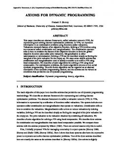
subject to the constraint (6) ∑ where Number of fire retardant resources defending the th asset at layer A key ingredient to a fire is the fuel source, without which a fire cannot burn. A fire typically consumes all fuel sources as it burns through the environment limiting the ability for subsequent fires to follow the same path. Once an asset is destroyed, all viable fuel paths towards the asset have been consumed. Based on this knowledge, the attack vector will not have any fires directed towards an asset that has been previously destroyed. A. Three Layer Approach In order to closely mirror the wildland fire environment, our scenario incorporates multiple layers of defense to thwart an attack. A fire must successfully elude three multiple defense attempts to effectively destroy the asset. Figure 1 depicts the three-layered defense approach.




Figure 1. Three Layer Defense. Asset is attacked by fire . Defense vector is selected to eliminate the attack in the first layer. If the defense could not eliminate the threat, the surviving attack fire moves into layer 2, and so forth. represents the attacking fire that successfully navigated through the three layers and reached the asset. The decision-making process of the defense vector at each layer is independent of one another. Each layer is supplied with the updated reduced state vector and attack vector. B. Receding Horizon Approach The problem takes the three-layer approach one step further to mirror the real-world situation. In a finite-horizon model5, an agent forgoes current rewards to optimize its reward after discrete steps. In subsequent steps, the agent makes decisions on steps until the reward is one step away. This approach assumes that the agent knows how far away the horizon appears for its decision making. A modification to the finite horizon is the receding horizon; the agent will continuously make decisions based on the horizon always appearing discrete steps away. The receding horizon is ideal for the wildland fire as the terminal stage of the scenario is unknown. The method creates a virtual continuous environment that attacks are initiated at discrete steps and the simulation continues until one of two situations is satisfied: the total number of fires is extinguished or the total number of resources is depleted. C. Exclusion of Burnt Land The majority of fire growth modeling techniques adheres to the same underlying principle shape of an ellipse, which under normal conditions grows based on Huygens’ Principle of wave propagation. Normal conditions for fire factors are spread, velocity, fuels, topography, etc., which are spatially and temporally constant, an assumption which is rarely true in the environment9.

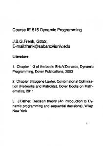
Figure 2. Fire Growth over Three Layers. The wildland fire is consuming fuel from the land as it approaches an asset and the area of the ellipse increases exponentially at each layer, listed as 1, 2, and 3 on the figure. Since the burning of land is a natural agent of change and at times encouraged through natural events and prescribed burns, the cost of land burned in the simulation is excluded. The top priority is to minimize the economical impact (loss of assets) and any land destroyed during the simulation is considered as a prescribed burn. D. Uncertainty Analysis In a perfect world, the information gathered would be complete and accurate, simplifying many of the constraints imposed on the problem. However, we must handle uncertainty within our system since error may be introduced due to the reliability of sensors. Three different uncertainty cases are explored: 1. Fire Error Percentage: The fire error percentage is the percentage increase in the number of fires over the estimated prediction. The control algorithms utilize the estimated number of fires to allocate resources accordingly throughout the simulation. The increase in fires will ultimately affect the results of the resource allocation. 2. Breakup Percentage: The breakup percentage is the possibility that a fire “jumps” and creates additional hotspots which occurs only at the third layer. An additional fire is added to the attack vector accordingly. 4 American Institute of Aeronautics and Astronautics


Page 4 of 20

Page 5 of 20


3.

False Alarm Percentage: The false alarm percentage is the possibility that a fire hotspot is rendered harmless in the third layer. The fire is removed from the attack vector accordingly. This information is unknown to the defender prior to the simulation. Any training or planning by the algorithms is based on the assumption of perfect knowledge of the environment. In event that a breakup or false alarm occurs in the third layer, the algorithms are responsive to the change in state and can react accordingly. E. Figures of Merit The figures of merit of the four control methodologies (greedy-based heuristic, DP, NDP, NFDP) are based on three parameters: execution time, remaining asset health, and scalability. The execution time quantifies the requirement of real-time decisions. The faster the execution time equates to a quicker reaction time to find the control policy. The remaining asset health is a measure of how well the control algorithm performed in protecting its assets from the attacker. The higher the remaining asset health results in a more successful control algorithm. Therefore, a promising algorithm is one where the execution is fast (sufficient for real-time decision-making) and a high remaining asset health. Finally, we examine the scalability of the system based on the complexity of its initial configuration. F. Scenario Description Five cases with initial attacker and defender inventories were setup for the simulation shown in Table 1. The predictive services10 program is a unit under the guidance of the National Predictive Services Subcommittee located throughout the United States at various NICC and GACCs establishments. The program “was developed to provide decision support information needed to be more proactive in anticipating significant fire activity and determining resource allocation needs…[and] consists of three primary functions: fire weather, fire danger/fuels, and intelligence/resource status information10.” It provides daily outlooks up to 3-month seasonal trend forecasts and aides in their short and long-term strategies for resource allocation. The predictive services function allows us to make some assumptions for the wildland simulation and construct initial inventories for the attackers and defenders:

Fires Layer 1 Case 1 2 3 4 5

15 15 15 15 15

3 4 5 3 3

3 5 5 3 7

1 1 1 1 1

Defense Resources Layer 2 3 5 5 5 7

1 1 2 1 1

Layer 3 3 5 5 8 7

2 2 2 2 2

Table 1. Test Case Setup The defense resources at each layer may only be used once per their assigned layer. After dropping their defense measure, they return to their respective base for service/restock and are readily available for the next mission task. In our scenarios, the attacker has targeted three distinct assets {asset 1, asset 2, asset 3}. The assets have initial property values of {5, 10, 15} and total health values of {5, 5, 5}. The initial asset health of the entire system is valued at 30 points calculated using Eq. (1). The calculation is a mathematical equation that is essentially dimensionless, points is a meaningless term to fill in the unit’s placeholder. Asset 1

Asset 2

Asset 3

(7)

In discrete time steps, the attacker will randomly attack assets. The simulation continuously runs until either all assets are destroyed or all fires have been extinguished.




Page 6 of 20

III. Methodologies The first three algorithms are based on the TMD problem by Bertsekas4, followed by the NFDP approach which extends Bertsekas’ work. A. Greedy-based Heuristic The premise of the greedy-based heuristic approach is to give preference to the highest valued assets at all times; remaining assets are protected based on resource availability and property value. The algorithm strictly adhered to the design of Bertsekas with the exception of the multi-layered approach, which decisions of resource allocation at each layer are made independent of one another. Once a fire is detected in a particular layer, the algorithm inventories the current state of the assets prioritizing the assets based on property value. The heuristic matches onefor-one every attack with a defense for the current highest property valued assets. If the number of remaining defense resources is greater than the expected number of remaining fires, then the surplus of defense resources are used on lower valued assets in decreasing order matching every attack with one defense. Otherwise, no further defense allocation is made. B. Dynamic Programming (DP) Dynamic programming lends itself well to multi-stage decisions where there is a tradeoff between the current state’s cost and future state’s cost2. In addition, DP is considered as the gold standard with respect to performance because it allows us to obtain the optimal solution, albeit at a huge computational cost. The underlying theory is Bellman’s Principle of Optimality: an optimal policy has the property that whatever the initial state and initial decision are, the remaining decisions must constitute an optimal policy with regard to the state resulting from the first decision3. The problem is cast as a Markovian decision process, such that ( )( ) ( ) represents the probability that the new state will be ( ) given the current reduced state, attack vector and defense vector. A Markov chain describes the transition probabilities of the system, the probability that attack will occur given the current state . Since the problem is setup as a stochastic shortest path problem, then ̂( ) can be formulated as ̂( )

∑ ( |)

(

(8)

)

where ( ) is the optimal expected long-term cost starting at state ( ) and ( | ) is the conditional probability that the next attack is given the current state . With the reduced optimal cost, ̂( ), at reduced state , Bellman’s equation can be rewritten as ̂( )

∑ ( |)

{ (

)

̂( )|

}

(9)

where (

)

∑

(

()

( ))

(10)

Equation (10) represents the one time step cost. Thus, the goal is to find the defense vector that minimizes the expected long-term cost given the current state and attack vector . Since we know that the system will terminate in finite time (based on previous assumptions that at least one attacking fire will occur at each time point and, either the attacking fires are extinguished or the number of assets are destroyed), Bellman’s equation will converge to a unique solution, the reduced optimal cost ̂( ), for all states . The DP approach is complicated by the use of multiple layers of defense. The transition from state to state inherently includes substates that result from the engagement of defense resources against the attack at different layers but does not incur a cost, a previously noted assumption for DP that implies transition cost to be summative, i.e. a fire eluding a defense at any layer excluding the final layer has not reach an asset. The defense allocation is the composite of all the substate defenses selected; the layer defense allocations are dependent on previous layer engagement results and the expectations of future layer engagements. The defense vector selected at each layer is the composite that minimizes the expected cost at the end of the layer sequence. Figure 3 shows the substates that transition from state to state . 6 American Institute of Aeronautics and Astronautics


Page 7 of 20


Figure 3: State transitions with Substates

DP lacks the ability to make good decisions with the absence of a cost to transition through the substates. To overcome this issue, the cost to transition from state to state is distributed to the appropriate substates as if each is considered a one-layer approach. The control action selected is then based on the summation of the substates plus the optimal cost-to-go, adhering to the constraint that cost is summative. The DP algorithm is updated as:

̂( )

∑ ( |)

[ (

̂( )|

)

]

(11)

Theoretically speaking, Eq. (12) can be solved by classical methods by iterating over the equation such that the generated sequences ( ) will converge to the optimal cost ̂( ) for all states . ()

∑ ( |)

{ (

)

( )|

}

(12)

However, the solution by exact methods is computationally expensive due to the large number of states. To overcome this drawback, a series of Monte Carlo simulations are performed on scenario models to collect empirical data for the expected engagement result , given the current state , attack vector , and defense vector . This essentially allows DP to learn from observing its own behavior and eliminates the need to perform probabilistic analysis to create the Markov chain for transition probabilities. The Bertsekas’ TMD work is extended by decreasing the engagement probability to examine the sensitivity of the DP algorithm. We expect the performance of the DP algorithm to decrease provided that the number of Monte Carlo simulations does not change between the various engagement probabilities. Given a lower engagement probability permits more options of transition states as compared to a system that is (nearly) deterministic. For the DP to be trained properly, it must explore as many paths as possible to get an accurate expected value. This is not the case for deterministic systems as the expected value to transition from state to is static. To compensate for the need for DP to train more, the number of Monte Carlo simulations is increased for the lower engagement probabilities. C. Neuro-Dynamic Programming (NDP) The Neuro-Dynamic Programming algorithm is formulated based on the concept of reinforcement learning, the idea of “an agent that must learn behavior through trial-and-error interactions with a dynamic environment5”. The overall goal for the agent is to select a control policy such that it maximizes the long-run summation of the reinforcement signal. Learning can be accomplished through systematic trial-and-error algorithms as in reinforcement learning, or by methods such as back-propagation as in Artificial Neural Networks (ANNs)5. The NDP algorithm focuses on approximating the reduced optimal cost function ̂( ) from Eq. (9) with a suitable ̃( ) by utilizing ANNs. The variable is a vector of parameters used in conjunction with the future state to approximate the cost-to-go function4. In this case, the parameters are the synaptic weights and the thresholds of the artificial neural network. The approximation produces sub-optimal results as compared to the DP algorithm, but can significantly decrease execution time of the algorithm. We utilized a fully-connected, feed-forward ANN designed specifically for this scenario. The number of inputs is based on the size of the reduced state vector depicted in Figure 4. The network contains eight neurons within one hidden layer and one neuron for the output.




Page 8 of 20

Figure 4. Fully Connected ANN with 7 Input Neurons, 8 Hidden Neurons, and 1 Output Neuron. All the neurons in the network utilize a symmetrical sigmoid function6 for the activation function: (13)

( )

where represents the input into the neuron. The neural network is trained using approximate policy iteration using Monte Carlo Simulations by iterating a predefined amount over the following four steps. Figure 5 shows an illustrated view of the cyclical training process.

Figure 5. ANN Training Process. 1.

Neural Network Approximator The weight matrix is initialized with random weights and the neural network generates values for the cost). to-go function ̃(

2.

Policy Update The optimal control policy is obtained based on the generated cost-to-go values from the ANN, by the following equation: ̅(

)

{ (

)

̃(

)|

}



(14)

Page 9 of 20


3.

Monte Carlo Simulations An initial reduced state is randomly created and all possible attack vectors are generated for that state. The optimal policy in step 2 generates the defense vector for every ( ) pair. The simulation continues the scenario generating defense vectors for every ( ) pair until a terminating state is reached. Sample costs are calculated from the equation: ∑ ( |)

()

{ (

)

̂( )|

̅(

)}

(15)

The combination of the reduced state and its respective sample cost represents the training set used for training the neural network. The Monte Carlo simulations are executed multiple times such that a sufficient training set is generated for training. 4.

Neural Network Training The collection of inputs-outputs from step 3 is used to batch train the neural network with the goal of minimizing the error between the output of the neural network and the sample costs. Training is the means by which the algorithm learns from its own behavior. The learning algorithm uses back-propagation by the gradient descent method and since the gradient descent method requires differentiating the activation function to minimize the error function, the sigmoid function guarantees continuity and differentiability 12. The neural network trains the nets up to 500 times with the batch training data; training is prematurely interrupted if an error ratio tolerance of 0.15 is met for 10 consecutive training steps. The following equation is used to adjust the weights of the network by minimizing the squared error: ()

(16)

∑ ∑ |̃ (

)

(

)|

After completion of neural network trainer, the NDP algorithm is primed for production use. Although it takes time to train the ANN, the process listed above is completed offline so that the parameter vector is adjusted accordingly; subsequently, the ANN becomes a ‘fixed network’ once simulation runs are executed. Since the ANN is trained offline, the training time is removed from the execution time of the simulation. D. Neuro-Fuzzy Dynamic Programming (NFDP) The NDP algorithm assumes complete knowledge of the environment with a heavy emphasis on the maximum number of wildland fires in the environment. Removing these assumptions introduces a new complexity to the problem, uncertainty to our inputs that the prior algorithms DP and NDP struggle to cope with during simulations. The NFDP algorithm seeks to minimize the impact of the uncertainty by providing robustness in the system. The NDP algorithm maintained a single ANN across all layers. The NFDP approach distributes three instances of the neural network at each layer. Although the decision of each ANN is made independent of one another, they must cooperate and make decisions to achieve their overall goal of minimizing the cost function. The one step cost function defined previously in the DP and NDP algorithms is the expected cost of assets destroyed during that time period. By distributing the neural networks to each layer, the one step cost must represent the combined cost of the three layers since a fire causes no damage until it eludes the last layer of defense. Therefore, the one step cost defined in Eq. (10) is modified to incorporate the uncertainty in the system and implementation of the multi-layer cooperation. The fuzzy term is used to estimate the contribution of the step cost at each layer. (

)

∑

(

()

( ))

where The normalized weight is defined as



(17)


Page 10 of 20

(18) ∑ Output of the fuzzy controller The defense resources must be used effectively given that the estimate of the maximum number of predicted fires may be inaccurate. The inputs and rule-base for the fuzzy inference system (FIS) are based on the rules of engagement in the Strategic Defense Initiative and terminal phase Arrow interceptor system 7. The framework is based on the theater missile defense and the transition to the wildland fire scenario is mostly transparent as the concepts of the two are similar. The NFDP algorithm employs a multi-input, single-output Sugeno FIS shown in Figure 6.

Figure 6. Block Diagram of Fuzzy Controller The ND input represents the normalized distance of the fire in relation to the asset. The AI input is the asset importance calculated in Eq. (19). The value is adjusted to fit in a range from 0.85 to 1.00. (

)

(19)

Each input consists of five membership functions based on sigmoid and Gaussian distributions.

Figure 7. ND Membership Functions

Figure 8. AI Membership Functions

The rule base is the application of heuristic rules in a series of IF-THEN statements to specify the output of the FIS. Each rule is a unique combination of the two inputs resulting in a total of 25 rules.



Page 11 of 20


ND (Normalized Distance) Mid Near Slightly Light Medium Slightly Light Medium Medium Slightly Very Medium Medium Medium Very Slightly Medium Medium Heavy Very Slightly Heavy Medium Heavy

AI (Asset Importance)

Very Far Very Low

Zero

Low

Very Light

Medium

Light

High

Slightly Medium

Very High

Medium

Far Very Light

Very Near Medium Very Medium Slightly Heavy Heavy Very Heavy

Table 2. Rule Base for NFDP Algorithm The Sugeno FIS output functions are characterized as crisp values:

Output Membership Function

Value (zj) 0.00

Zero Very Light Light

0.25

Slightly Medium Medium Very Medium Slightly Heavy Heavy Very Heavy

0.50 0.75 1.00 1.25 1.50 2.00 3.00

Table 3. Output Membership Functions for NFDP Algorithm The defuzzification stage converts the rule base results into a final crisp output value. The output level of each rule is weighted by the fire strength of the rule. The final output of the FIS is the weighted average of all rule outputs computed as ∑

(20) ∑

where The total number of rules The weight of the rule The output level at the rule

IV. Results The results are grouped into four categories based on the certain and uncertainty scenarios. Within each scenario are two tables depicting the remaining asset health and execution time of the five test cases. The accompanying 11 American Institute of Aeronautics and Astronautics



Page 12 of 20

graph is a visual illustration of the average values. Due to the large range of execution time values, the y-axis is in logarithmic scale. The preferred methodology should approach the bottom right corner of the graph encompassing both high remaining asset health and low execution time. A. Sensitivity to Engagement Probability The system would be considered a deterministic system if the engagement probability of the defense resources were 1.0. An area of interest is how the performance would be impacted due to varying degrees of engagement probability. Since the Dynamic Programming approach provides the optimal and benchmark results, only the DP approach was used to evaluate this area. In all cases, the simulations were simulated under the same conditions with three different engagement probabilities of 0.9, 0.8, and 0.7.

Remaining Asset Health 0.9 0.8 0.7 21.80 19.80 16.80 27.50 23.80 24.10 27.80 24.80 23.60 28.10 27.10 24.30 29.50 28.50 27.40 26.94 24.80 23.24

Case 1 2 3 4 5 Average

Table 4: Sensitivity – Remaining Asset Health It would be expected that low scenarios where engagement probabilities were more stochastic would result in poorer performance. To counter the decreased engagement probability, the number of Monte Carlo simulations was increased to allow the DP to train better from observing its own behavior. The adverse effect to achieve similar results by increasing the Monte Carlo simulations was the increased execution time, as evident in Table 5.

Case 1 2 3 4 5 Average

0.9 375 5,243 9,770 4,780 31,193 10,272

Execution Time (s) 0.8 0.7 978 2,742 16,651 41,739 40,346 111,641 17,286 37,460 90,281 216,938 33,108 82,504

Table 5: Sensitivity - Execution Time (s) Due to the large amount of time to run simulations for 0.8 and 0.7 engagement probabilities, the remainder of the results is focused solely on the engagement probability of 0.9. B. Uncertainty Analysis No Uncertainty The no uncertainty case assumes the defender has complete knowledge of the environment, is fully informed of the number of fires, and all decisions are based on this knowledge. Case

Heuristic

NDP

NFDP

DP

1

18.15

18.60

18.25

21.50

2

23.93

24.68

25.29

27.50

3

23.17

25.38

24.50

28.40

4

24.43

27.19

25.46

28.40



Page 13 of 20


5

28.32

29.20

29.04

28.80

Average 23.60 25.01 24.51 26.92 Table 6. No Uncertainty: Remaining Asset Health.

Case

Heuristic

NDP

NFDP

DP

1

0.055

0.015

0.078

86

2

0.065

0.071

0.055

1,790

3

0.035

0.179

0.066

2,851

4

0.043

0.072

0.094

1,495

5

0.047

0.190

0.094

9,601

Average 0.049 0.105 0.077 3,165 Table 7. No Uncertainty: Execution Time.

Figure 9. No Uncertainty: RAH vs Execution Time.

Fire Error 20% The fire error represents the percentage increase in attacking fires unbeknownst to the defender. The decision making process of the defender will be based on its estimated number of fires and not the true amount. Case

Heuristic

NDP

NFDP

DP

1

16.40

16.10

15.49

16.00

2

22.10

22.31

23.67

23.80

3

21.87

22.16

23.47

21.60

4

23.34

23.35

23.94

22.40

5

26.99

28.00

27.89

28.60

Average 22.14 22.38 22.89 22.48 Table 8. Fire Error 20%: Remaining Asset Health. 13 American Institute of Aeronautics and Astronautics



Page 14 of 20

Case

Heuristic

NDP

NFDP

DP

1

0.068

0.016

0.094

13

2

0.037

0.095

0.067

1,414

3

0.034

0.195

0.072

2,624

4

0.045

0.089

0.079

1,376

5

0.068

0.016

0.078

10,613

Average 0.050 0.082 0.078 3,208 Table 9. Fire Error 20%: Execution Time.

Figure 10. Fire Error 20%: RAH vs Execution Time. Breakup 50% The breakup percentage is the number of fires that will jump to create another burning hotspot in the landscape when entering the third layer. This information is unknown to the defender prior to the simulation, but we assume that it recognizes the fire jump and can account for the increase in fires. Case

Heuristic

NDP

NFDP

DP

1

15.49

12.50

15.20

17.40

2

20.26

20.29

22.16

23.70

3

20.46

20.42

22.15

23.10

4

21.51

21.94

19.89

22.90

5

26.20

25.20

27.54

27.80

Average 20.79 20.07 21.39 22.98 Table 10. Breakup 50%: Remaining Asset Health. Case

Heuristic

NDP

NFDP

DP

1

0.063

0.010

0.094

124

2

0.096

0.065

0.082

1,654

3

0.049

0.168

0.107

2,848

4

0.052

0.072 0.061 1,809 14 American Institute of Aeronautics and Astronautics


Page 15 of 20


5

0.068

0.016

0.078

11,709

Average 0.065 0.066 0.084 3,629 Table 11. Breakup 50%: Execution Time.

Figure 11. Breakup 50%: RAH vs Execution Time. False Alarm 50% The false alarm percentage represents the number of fires that are rendered harmless due to natural occurring events (loss of fuel, change in environmental conditions, natural fire barrier, etc). Case

Heuristic

NDP

NFDP

DP

1

23.81

26.50

24.28

25.60

2

26.96

29.27

28.06

29.06

3

26.96

28.87

28.00

29.00

4

27.39

29.30

28.83

29.60

5

29.44

30.00

29.62

30.00

Average 26.91 28.79 27.76 28.65 Table 12. False Alarm 50%: Remaining Asset Health. Case

Heuristic

NDP

NFDP

DP

1

0.067

0.015

0.078

111

2

0.062

0.111

0.070

1,543

3

0.059

0.218

0.097

3,394

4

0.047

0.067

0.046

1,573

5

0.569

0.016

0.078

11,570

Average 0.161 0.085 0.074 3,638 Table 13. False Alarm 50%: Execution Time.




Page 16 of 20

Figure 12. False Alarm 50%: RAH vs Execution Time. Summary Results for All Scenarios Table 14 and Table 15 display the average results over all scenarios and the average over all uncertainty scenarios. Heuristic

NDP

NFDP

DP

No Uncertainty

23.60

25.01

24.51

26.92

Fire Error 20%

22.14

22.38

22.89

22.48

Breakup 50%

20.79

20.07

21.39

22.98

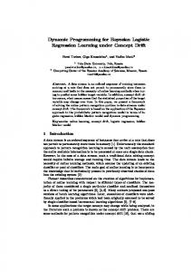
False Alarm 50% 26.91 28.79 27.76 Average Results of 23.28 23.75 24.01 Uncertainty Cases Table 14: Summary – Remaining Asset Health

28.65

Heuristic

NDP

NFDP

DP

No Uncertainty

0.049

0.069

0.077

3,165

Fire Error 20%

0.050

0.082

0.078

3,208

Breakup 50%

0.065

0.066

0.084

3,629

False Alarm 50% 0.161 0.085 0.074 Average Results of 0.092 0.078 0.079 Uncertainty Cases Table 15: Summary – Execution Time (s)

3,638



24.70

3,492

Page 17 of 20


Figure 13: Comparison of Results for Uncertainty Scenarios

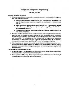
C. Scalability The final metric of interest is the scalability of the approaches shown in Figure 14. The DP increases a couple orders of magnitude as the complexity of the system increases as opposed to the other methods.

Algorithm Scalability to System Complexity Execution Time (s)

10,000.00 1,000.00 Heuristic

100.00

NDP

10.00

DP

1.00 1

0.10

2

3

0.01

4

5

NFDP

Case Figure 14: Scalability to System Complexity

The DP algorithm does not scale well with increased complexity as expected. To facilitate a better understanding of how the how methods scale, an additional test case of higher complexity is included (the DP algorithm is excluded from the results.

Fires Layer 1 Case 6

22

4

8

2

Defense Resources Layer 2 8

2

Layer 3 8

2

Table 16: Additional Test Case for Scalability Figure 15 provides a better representation of the execution time to system complexity for the heuristic, NDP and NFDP algorithms. 17 American Institute of Aeronautics and Astronautics



Page 18 of 20

Execution Time (s)

Algorithm Scalability to System Complexity (sans DP) 1.00 1

2

3

4

5

6

0.10 0.01

Heuristic NDP NFDP

Case Figure 15: Scalability to System Complexity (sans DP)

V. Conclusion There are three key areas of interest for this paper: sensitivity to various engagement probabilities, ability to handle uncertainty, and scalability. Bertsekas et al.4 used an engagement probability of 0.9 for the TMD problem, a probability that can be considered realistic for purposes of the problem. It is difficult to find literature or any acceptable agreed upon probability of using fire retardants to extinguish a fire although understandably will be anything less than 1.0. The results are based on the 0.9 engagement probability for two reasons; first, to compare the benchmarks cases with Bertsekas and second, to provide a solid foundation to implement a fuzzy logic component. To supplement a study in lower probabilities of engagement, this paper explored the results solely for Dynamic Programming for probabilities of 0.9, 0.8 and 0.7. The expected outcome is a decrease in performance (remaining asset health) when engagement probabilities are lower; a higher chance that a fire escapes a defense. The results subsequently show the decrease in performance. Initial tests of the sensitivity without changing the amount of learning performed (i.e. Monte Carlo simulations) resulted in a larger depreciation of results such that the simple greedy-based heuristics outperformed the DP which intuitively should not occur. The DP minimizes the expected value of the one step cost plus optimal cost-to-go. The 0.9 probability case does not require an extensive amount of Monte Carlo simulations to find the expected value. State will transition to based on the control policy ; given that the 0.9 case is nearly-deterministic, it is not necessary to execute numerous Monte Carlo simulations since there will not be a lot of differing states. A total of 15 Monte Carlo simulations were found to be suitable to calculate the expected value. However, as the engagement probability decreases, the number of possible states increases and 15 Montes Carlo simulations does not sufficiently explore all the additional states for a suitable expected value. To overcome this drawback, the number of Monte Carlo simulations is increased to 30 and 60 for the 0.8 and 0.7 cases, respectively. The increase permits the DP to explore more subsequent states for a better estimation of the expected value. The results in Table 4 show the smaller decrease in remaining asset health for the various engagement probabilities as expected. The drawback for increasing the number of Monte Carlo simulations is seen in Table 5. The execution time needed to improve the DP learning greatly increases the time for a suitable solution, an unacceptable byproduct of the lower engagement probabilities. The second metric is the performance of the various algorithms to varying levels of uncertainties along with the benchmark case of perfect knowledge of the system. The ‘no uncertainty’ case ensures the design sufficiently correlates with the work by Bertsekas et al. and further provides a solid foundation to compare results for the uncertainty cases. The sensitivity analysis provided insightful information on the execution time of the DP approach. The NDP and NFDP algorithms have substantially faster execution times but do not reflect the required offline training performed by means of a DP simulation. To expedite the process of gathering results for the DP, NDP, and NFDP, the DP algorithm was tested with fewer Monte Carlo simulations and found that seven Monte Carlo simulations to calculate the expected value improved the execution time with minimal impact on the results. The DP provided the average optimal result for all cases at a huge computational cost, two orders of magnitude longer than the other approaches. On the other hand, the greedy-based heuristic using linguistic rules had the best execution time since it simply evaluates the current state of the system without any mathematical optimization or dependence on future states. Subsequently, this approach results in the worst performance. The performance of the NDP and NFDP for remaining asset health and execution were similar. Each had quick execution time by approximating the cost-to-go function but suffered the cost of poorer performance for that approximation. However, the decrease in remaining asset health was minimal for the reward of quicker execution time. Excluding the NFDP 18 American Institute of Aeronautics and Astronautics


Page 19 of 20


algorithm since this option was not explored in the Bertsekas TMD paper, the results of the greedy-based heuristic, NDP and DP algorithms were sufficient and solidified the current work. Three uncertainty cases were explored for this paper: an increase in the number of fires in the simulation, the probability of fires breaking up in the third layer and creating new fires, and the probability of a fire being rendered harmless naturally in the third layer. This information is unknown to the optimization algorithms prior to their execution. In two of the three uncertainty scenarios, the DP algorithm failed to handle the unknown information and resulted in weaker remaining asset health performance. Essentially, the DP utilized its defense resources on lower valued assets with its own expectation of the number of remaining fires resulting in poor decision-making. However, its strong performance in the false alarm scenario was able to over the deficiencies to have the best overall remaining asset health performance for the uncertainty scenarios. In all three cases though, the execution time of the DP again eliminates the approach as a feasible real-time decision tool. The objective of the NDP algorithm was to reduce the computational costs of DP by training an artificial neural network to approximate the optimal cost-to-go function and the NDP was trained without any knowledge of uncertainty. NDP results were affected by the uncertainty but not nearly to the same effect as DP. The NFDP performed the best of the real-time decision making algorithms for the uncertainty scenarios. The fuzzy logic component incorporated into the one step cost function provided robustness in the presence of uncertainty. By using linguistic reasoning, the one step cost is weighted by the fuzzy controller to aid in the decision-making, effectively making better decisions. Additionally, whereas NDP makes decisions on the collective effort of the three layers of defense, NFDP decouples local decision-making permitting a more consistent execution time across the different cases even as system complexity increases. The results of the uncertainty call for two additional areas of recommended research. First, how the NDP and NFDP would perform under lower engagement probabilities based on the same uncertainty analysis. Second, introduce another uncertainty where the engagement probability is uncertain and may vary in a range of plus or minus 0.1. The control algorithms would be trained based on an assumed value but encounter various engagement probabilities during simulation. The final metric is the scalability of the algorithms to system complexity due to increased defense resources and fires in the scenario. The increased size of resources and fires requires more resource allocation tasks and decisions to be made. The cases are ordered in terms of increasing complexity (cases 2 through 4 can be considered roughly the same in terms of complexity). The DP algorithm fared the worst of the algorithms with increases on the order of magnitudes in time. The DP explores all feasible states to find the optimal control policy, prompting a significant increase in execution time to explore those possible states. This is inherently true for the training of the NDP and NFDP algorithms but since those algorithms are trained offline, the execution time is not reflected in the final online simulation time. The execution times of NDP and NFDP remained relatively stagnant since cost-to-go values are computed utilizing approximation methods. The NFDP appears to fare slightly better in scalability since decisions are made locally at each layer whereas NDP still relies on the collective decision-making between the layers requiring more time and decisions. It is recommended to execute additional test cases with sizable increases in complexity to statistically confirm this conclusion. The development of this paper was its intended use as a decision support system during wildland fires. FARSITE11 is a commonly used fire growth and behavior simulation tool used to simulate wildland fires and evaluate their characteristics. In addition, users can make decisions on various defense mechanisms and evaluate their effectiveness at the conclusion of the simulation. What FARSITE lacks is an innovative decision support system to complement the simulation tool. The decision algorithms defined in this paper, in particular NFDP, would allow users to execute simulations utilizing this tool to make optimal or near optimal decisions on the allocation of their resources. This paper lays the groundwork for the decision making tool but would require further enhancements for a FARSITE integration. First, this work is developed as a linear system and requires an extension to the spatialtemporal FARSITE environment. Therefore, the optimization algorithm must account for spatial position of its resources and timing. Second, this approach uses a three-layered defense (three step horizon). The FARSITE model permits a larger horizon from which decisions are made. The DP algorithm shows its inability to provide real-time execution while the NDP and NFDP approaches were promising algorithms. However, since the change to a spatial-temporal environment and larger horizon requires more possible control options to evaluate and further look ahead render the NDP as an infeasible option. Recall, the NDP approach’s scalability may become an issue as the complexity of the scenario increases since the NDP layers rely on the choices made at each layer. It is envisioned that the algorithm integration is formulated as a feedback loop. The FARSITE simulation will progress one time step and the NFDP algorithm makes a control decision given the perception of the environment, estimating the cost of one time step plus the approximated cost-to-go. Since decisions are made locally at the layer, 19 American Institute of Aeronautics and Astronautics



Page 20 of 20

the decision is made in real-time and the control action is fed into the FARSITE model. This process continues until an ending state is reached. Given such a large solution space, it can be overwhelming to a user to find the optimal allocation of resources. In addition, the knowledge captured during simulation is retained by the user and it can be difficult to transfer that knowledge to other users. The decision support tool extracts that knowledge and allows the user to focus on other tasks. Thus, users are able to simulate a fire and utilize the decision making algorithms to aid in the allocation of resources. Additionally, as FARSITE is a visual simulation tool, this feature allows users to visually watch and evaluate the effectiveness of the control algorithm.

Acknowledgments We would like to thank Dr. Praveen Chawla and EDAptive Computing, Inc. for their support in this project.

References 1

Mandel, J., Chen, M., Franca, L. P., Johns, C., Puhalskii, A., Coen, J. L., Douglas, C. C., Kremens, R., Vodacek, A., and Zhao, W., A Note on Dynamic Data Driven Wildfire Modeling, Springer-Verlag, 2004, pp. 725-731. 2 Bertsekas, D. P., Dynamic Programming and Optimal Control, 3rd ed., Vol. 1, Athena Scientific, Belmont, 2005. 3 Bertsekas, D. P., and Tsitsiklis, J., Neuro-Dynamic Programming, Athena Scientific, Belmont, 1996. 4 Bertsekas, D. P., Homer, M. L., Logan, D. A., Patek, S. D., and Sandell, N. R., “Missile Defense and Interceptor Allocation by Neuro-Dynamic Programming,” IEEE Transactions on Systems, Man and Cybernetics, Vol. 30, No. 1, 2000, pp. 42-51. 5 Kaelbling, L. P., Littman, M. L., and Moore, A. W., “Reinforcement Learning: A Survey,” Journal of Artificial Intelligence Research, Vol. 4, 1996, pp. 237-285. 6 Rojas, R., Neural Networks A Systematic Introduction, Springer, Berlin, 1996. 7 Naveh, B., Levy, E., and Cohen, K., “Theater Ballistic Missile Defense Architecture Development,” Theater Ballistic Missile Defense, AIAA, Reston, 2001, pp. 77-97. 8 Walch, B., “The Fire This Time,” TIME, November 2007, pp. 14-17, [http://www.time.com/time/classroom/glenspring2008/pdfs/Nation.pdf Accessed 6/10/10.] 9 Finney, M. A., “Rocky Mountain Research Station”, US Forest Research and Development, March 2004, [http://www.fs.fed.us/rm/pubs/rmrs_rp004.html Accessed 2/20/09.] 10 National Interagency Coordination Center. GACC >Predictive Services. National Interagency Fire Center. [Online] http://www.predictiveservices.nifc.gov/predictive.htm. 11 Missoula Fire Sciences Laboratory. FARSITE. FireModels.org Fire Behavior and Fire Danger Software. [Online] July 20, 2009. http://firemodels.fire.org/content/view/112/143/. 12 Rojas, Raul. Neural Networks A Systematic Introduction. Berlin : Springer, 1996.



Neuro-Fuzzy Dynamic Programming for Decision

Neuro-Fuzzy Dynamic Programming for Decision

Suggest Documents

Dynamic Programming for Structured Continuous Markov Decision

Dynamic programming and Markov decision ... - Herd Management

markov decision processes: discrete stochastic dynamic programming ...

Dynamic programming in constrained Markov decision processes

Faster Dynamic Programming for Markov Decision ... - Semantic Scholar

Axioms for Dynamic Programming

Approximate dynamic programming for

Nonlinear Programming Method for Dynamic Programming

Offline-Online Approximate Dynamic Programming for Dynamic

Dynamic Programming

Dynamic programming

Dynamic Programming

Approximate Dynamic Programming for Communication ...

Sparse Approximate Dynamic Programming for

Dynamic Programming for Bayesian Logistic

Study Guide for Dynamic Programming

Neurofuzzy Modelling - Semantic Scholar

Dynamic Programming as a Tool of Decision Supporting - aensi

Neurofuzzy Modelling - Semantic Scholar

Decision support for real-time, dynamic decision-making tasks

Dynamic Decision Networks for Decision-Making in Self ... - CiteSeerX

Evolutionary Reinforcement Learning for Neurofuzzy Control - CiteSeerX

Chapter 15: Dynamic Programming

Dynamic Programming Strikes Back