NeuroHough: A Neural Network for ... paradigm makes use of the neural networks' properties as function ... particular case of the mathematical transformation.
NeuroHough: A Neural Network for Computing the Hough Transform M.Köppen, A. Soria-Frisch, R. Vicente-García Fraunhofer IPK, Dept. Pattern Recognition, Pascalstr. 8-9, 10587 Berlin, Germany
Abstract. A new paradigm for the implementation of the Hough Transform (HT) is presented in this paper. The paradigm makes use of the neural networks' properties as function approximators in order to avoid some problems of the standard HT implementation. Some encouraging results are presented.
1 Introduction Originally designed as a procedure to detect patterns on binary images [8] the Hough Transform (HT) is nowadays a methodology used for the resolution of a wide variety of problems in image processing and understanding. Beyond the classical application for linking contours on edge maps [5] the HT is applied in object recognition [6], shape parametrization [11][12], shape detection [13][17], and movement analysis on image sequences [4]. The performance of the original HT has been improved with the apparition of numerous modifications, e.g. generalized HT [2], adaptive HT [9], fast HT [14], randomized HT [16], fuzzy HT [7], whose abundance can be taken as a sign of its regard as processing tool. Moreover the research on the subject has been encouraged by the uncertain classification of the HT from a theoretical point of view. The HT has been considered as a paradigm of a more general connectionist model for low- and intermediate-level visions [3]; as a product of Bayes theorem [18]; as an evidence gathering procedure in the context of a computational evolutionary strategy [15]; and as a particular case of the mathematical transformation called Radon transform [19]. The here presented paradigm does not want to bring this fruitful tradition to an end but to widen it into the theoretical framework of neural networks. This point was scarcely considered in [3] and [18]. In this case the paradigm makes use of a neural network as function approximator, a new terrain for the implementation of the HT. A brief review on the HT is presented in Section 2. In Section 3 the neural architecture is discussed. Finally
some results, the conclusions and the projective work can be found in Section 4.
2 The Hough Transform on review The HT considers the transformation of the image space to a multidimensional parameter space, where a set of image points (x,y) belonging to a determined geometrical element in the image space is represented by a combination of its characterizing parameters. This parameter space consists of a set of discrete accumulator cells, which are incremented when a point in the image space fulfills the analytical expression of the geometrical element being searched for. In this socalled accumulation process the fulfillment of the analytical expression acts as a piece of evidence being accumulated in the parameter space. The parameter space is finally analyzed to detect the cells where the evidence is mostly accumulated. Therefore the geometrical element can be characterized as a function of the parameters related with the most voted accumulator cell. In the most basic application of the HT a straight line is for instance characterized through the length (ρ) and orientation (θ) of its normal vector: f (( x, y), ( ρ ,θ )) = ρ − x cos θ − y sinθ = 0 (1) In this case the parameter space is two-dimensional and the straight line is eventually parameterized through (ρ,θ) of the accumulator cell with a greatest value (characterization that includes the error produced by the discretization of the parameter space). The generalization of the HT for the detection of arbitrary shapes was introduced by Ballard [2]. The generalizing strategy is to increase the dimensionality of the parameter space in order to include not only changes in the geometrical element to be detected, but also in its translation, scale and rotation. 2.1 Properties of the HT for shape detection The HT has demonstrated its suitability for the detection of shapes on edge maps [13][17]. This
suitability is based on the reduction of the complex problem of line analysis to a more tractable one of peak detection in the parameter space. This is true even for the detection of arbitrary shapes, thanks to the already mentioned generalized HT. The robustness of the HT in front of noisy images, light deformations of the searched shapes respect to its model, and discontinuities of some parts of the edges are very appreciated features of this kind of analysis. Another interesting property is the parallelism of the computations undertaken in the calculation of the HT. The analysis of a complex form can be carried out after a decomposition in simpler geometrical elements of the model shape. Moreover the structure of the accumulator cell allows also the parallelization of this computation for each line. This property has been exploited in numerous parallel architectures implementing the polar parameters finding approach [10], and even in a general connectionist framework for modeling low and intermediate human vision [3]. 2.2 HT drawbacks The extensive memory usage and the computational cost, both proportional to the dimensionality of the parameter space, are the most known disadvantages of the HT for shape detection [10]. The problem of computational cost becomes more evident when trying to detect complex forms or to implement the methodology in applications where real-time response is needed. Beside this, quantization errors appear when applying the methodology in real applications due to the consideration of a discrete parameter space. In order to successfully implement the methodology a trade-off is needed [1]. Parameter accuracy on the one hand, and computational time and tractability of 'thick' lines (see figure 1) on the other have to be considered.
The apparition of false peeks is a minor problem when considering the HT from a mathematical point of view, but plays an important role in the resolution of real problems. They appear in front of spurious edges and of aligned points of objects that are separately analyzed, and due to reflective adjacency relationships of lines occupying extreme positions in polar accumulator spaces [5] (see figure 1). 2.3 Neural Networks Solution In the following a neural network paradigm for the computation of the HT, which will be called NeuroHough Transform, will be presented. The purpose of this implementation is the avoidance of some drawbacks of the classical implementation taking advantage of the approximation capability of neural networks. One of the general goals to be attained through the neural implementation of the HT is the constancy in terms of computation time independently from the complexity of the analyzed shape and the quantization step of the parameter space. This is a significant point when trying to implement the HT in real-time. The neural implementation should be also easier to generalize, what will allow the analysis of more complex scenes than edge maps, i.e. the analysis of surfaces and textures. Finally the NeuroHough Transform is thought to achieve the elimination of some false peeks, those caused by adjacency reflection and by the presence of spurious contours, through usage of pre-processed training data. Being these goals quite ambitious the main objective of the here presented work was succeeding in implementing the HT through a neural network.
3
1a 1b Fig. 1: Hough Transform pair that show different notdesired effects in the parameter space (1b). Lines A and B in the image space (1a) should appear as unique points A and B in the parameter space (1b). B appears not as a point but as a surface, due to the thickness of the line in image space (1b). The same as C, which is a point induced by a reflective adjacency relationship with B. The cloud of points D, caused by alignments of different points in lines A and B (1a), avoids a clearer appearance of point A in the parameter space (1b).
NeuroHough Transform
In this section, a method is proposed to represent the computations of the HT by a neural network. The proposed architecture can be observed in figure 2. Some previous aspects have to be taken under consideration before realizing the neural architecture. Assume the HT constructed from a mapping H of the four-tupel (x,y,ρ,θ) into the interval [0, 1] , with x and y coordinates in the image space and ρ and θ the coordinates in the accumulator space. Thereby, the assignment H(x,y,ρ,θ)=1 means that the presence of the pixel (x,y) in the image foreground domain induces the accumulator cell with the coordinates (ρ,θ) to be incremented by 1. For H(x,y,ρ,θ)=0, the accumulator cell remains unchanged. Thus, the HT is realized by
going for each (x,y) in the image foreground over all (ρ,θ) according to the chosen quantization of the accumulator space, and adding H(x,y,ρ,θ) to the corresponding cells: (2) A( ρ, θ ) = H( x, y, ρ ,θ )
∑
(x , y) in I
This will give the same result as for the standard Hough transform algorithm, but can be computed cell-wise. Now, the task for the neural network is to approximate H(x,y,ρ,θ). For the function approximation no special neural architecture is necessary and thus a 3-layer Backpropagation Network was chosen for the sake of simplicity. However a special representation of the given input and output data is considered. Image Space (x,y)
Multilayer Neural Network
Parameter Space Accumulator
Sweep
( ro , theta )
Fig. 2. Proposed neural architecture for the computation of the HT, NeuroHough.
The neural network is fed with the following input data: x, y, x*sinθ, y*cosθ, ρ, sinθ. This is regarded to the fact that neural networks may have problem to internally approximate products of input data. Furthermore the inclusion of redundant inputs help to empirically adjust the relevance of the input parameters. So, for the standard Hough transform, the task is presented as a linear separation problem to the network. For the output, two neurons are used. Considering the Hough equation, as in (1), it could be assumed that the neural network should compute the value 0 for "correct" (x,y,ρ,θ) tupels (and "non-zero" otherwise) just using one output neuron. However, this approach is not practicable, since the training data become ambiguous. It is simpler to train a network on having either output value larger or smaller than a given threshold (due to the sigmoidal transfer functions used). So, for the "neural computer", a=0 is taken as (a>=0) AND (a 0: O1=1, O2=0, II. ρ-x sinθ-y cosθ < 0: O1=0, O2=1, III. ρ-x sinθ-y cosθ = 0: O1=1, O2=1 (the case O1=O2=0 never happens).
As a consequence the NeuroHough network is trained by randomly selecting (x,y) positions and (ρ,θ) values, checking for case 1, 2 or 3 and setting accordingly the training data. The training set itself should be planned in a manner so that the loading of values 0 or 1 into the output neurons is balanced. This procedure will give a neural network, which is able to perform the computations of the standard HT and can be directly trained from the analytical expression of the transform. The same training procedure can be used for slight modifications of the transform, since it is based on a more general interpretation of the Hough transform not considered so far (as a special case of an arbitrary mapping of R4 into the interval [0,1]). For a superposed training regime, the NeuroHough procedure can be used for the initial configuration. Then, the error backpropagation procedure has to be modified according to the given recognition task. This is mostly addicted to further works on this approach. But before doing so, it is essential to prove the validity of the approach by representing the standard HT in its neural form.
4
Preliminary Results, Conclusions and Future Work
In order to approximate the desired function using a Multilayer Backpropagation Network the empirical performance of the paradigm was researched. The training and test data sets do not include any noise added and the amount is usually about 7000 examples.
3a
3b 3c Fig. 3: Hough Transformation of an image (3a) with the classical procedure (3b) and through the here presented neural network paradigm, NeuroHough (3c).
Till now the best results were obtained with a 3layer structure, 7 neurons in the input layer, 2 in the output one, and between 18 and 20 neurons in the hidden layer. Larger checked network sizes did not
improve the results significantly and needed very large training time, while smaller sizes underfit the targets. The gain is set to 3 in order to sharpen decision areas of the network, the momentum factor, the learning rate, and the initial weights were and to achieve a good generalization in a reasonable training time. The results obtained till now are excellent in terms of approximation capability. The Hough Transformation could be approximated through the NeuroHough, what can be observed in the case of the transformation of a straight line (see figure 3). The NeuroHough shows a good generalization capability, as the result (3c) were obtained with a neural network trained for the transformation of a line different from the one shown (3a).
shapes, which was one of the aims to be attained by the neural implementation of the HT, was reached through the implementation of the NeuroHough architecture (see figure 4c and 4e). Although having only been trained with straight lines the transformation of a circumference was encouraging (4f). The complete results of the here presented work, which is on progress at the present, will be presented in future communications.
References [1] [2] [3] [4] [5] [6]
4a
4b
[7] [8] [9] [10] [11]
4c
4d
[12] [13] [14] [15] [16]
4e 4f Fig. 4. Transformation of more complex forms through the here presented NeuroHough architecture. Original images of a square (4a) and a circumference (4b) were transformed with the classical HT (respectively, 4c and 4d) and the NeuroHough Transform (respectively, 4e and 4f). The suppression of points due to reflective adjacency relationship (4c) can be avoided using this methodology (4e).
Also the suppression of points due to reflective adjacency relationship in the analysis of more complex
[17]
[18] [19]
R.C. Agrawal, R.K. Shevgaonkar, S.C. Sahasrabudhe (1996). A fresh look at the Hough transform, Pattern Rec. Letters 17 (10) 1065-1068. D.H. Ballard (1981). Generalizing the Hough Transform to Detect Arbitrary Shapes, Pattern Recognition 13 (2) 111122. D.H. Ballard (1984). Parameter Nets, Artificial Intelligence 22, 235-267. I. Fermin, A. Imiya, A. Ichikawa (1996). Randomized polygon search for planar motion detection, Pattern Rec. Letters 17 (10) 1109-1115. R.C. Gonzalez, R.E. Woods (1993). Digital Image Processing, Addison-Wesley Pub. Co. W.E.L Grimson, D.P. Huttenlocher (1990). On the Sensitivity of the Hough Transform for Object Recognition, IEEE Trans. PAMI 12 (3) 255-273. J.H. Han, L.T. Kóczy, T. Poston (1994). Fuzzy Hough Transform, Pat. Rec. Letters 15 (7) 649-658. P.V.C. Hough (1962). A method and means for recognizing complex patterns, U.S. Patent 3,069,654. J. Illingworth, J. Kittler (1987). The Adaptive Hough Transform, IEEE Trans. PAMI 9 (5) 690-697. J. Illingworth, J. Kittler (1987). A Survey of the Hough Transform, Comp. Vision, Graphics, and Image Processing 44, 87-116. D. Ioannou, E.T. Dugan, A.F. Laine (1996). On the uniqueness of the representation of a convex polygon by its Hough transform, Pat. Rec. Letters 17 (12) 1259-1264. V.F. Leavers, J.F. Boyce (1987). The Radon transform and its application to shape parametrization in machine vision, Image and Vision Computing 5 (2) 161-166. V.F. Leavers (1992) Use of the Radon transform as a method of extracting information about shape in two dimensions, Image and Vision Comp. 10 (2) 99-107. H. Li, M.A. Lavin, R.J. LeMaster (1986). Fast Hough Transfor: A Hierarchical Approach, Comp. Vision, Graphics, and Image Processing 36, 139-161. J. Louchet (2000). From Hough to Darwin: An Individual Evolutionary Strategy Applied to Artificial Vision, Lecture Notes in Comp. Sci. (1829): Artificial Evolution, Springer. R.A. McLaughlin (1998). Randomized Hough Transform: Improved ellipse detection with comparison, Pattern Rec. Letters 19 (3-4) 299-305. D.C.W. Pao, H.F. Li, R. Jayakumar (1992). Shapes Recognition Using Straight Line Hough Transform: Theory and Generalization, IEEE Trans. PAMI 14 (11) 1076-1089. A.S. Rojer, E.L. Scwartz (1992). A Quotient Space Hough Transform for Space-Variant Visual Attention, Neural Networks for Vision and Image Processing, MIT Press. P. Toft (1996). The Radon Transform, Theory and Implementation, PhD Thesis, TU of Denmark.