In this paper we give an overview of some of the neuromorphic vision circuits that ..... time the selected zero-crossing (enforcing the a-priori assumption that the ...
Neuromorphic Vision Chips: intelligent sensors for industrial applications Giacomo Indiveri, J¨org Kramer and Christof Koch Computation and Neural Systems Program California Institute of Technology Pasadena, CA 91125, U.S.A. Abstract In the past years researchers at the California Institute of Technology (and in few other research institutions worldwide) have been concentrating their efforts on the design and implementation of analog VLSI neuromorphic systems. Today this emerging technology seems to be mature enough for use in industrial applications. In this paper we give an overview of some of the neuromorphic vision circuits that have been developed at the California Institute of Technology. To point out the advantages and disadvantages of using these types of circuits in industrial applications (with emphasis on the automotive market), we describe a system implemented on a single chip, that detects the direction of heading in the case of translatory ego-motion in a stationary environment. This device contains a variety of analog circuits typically used in neuromorphic systems. We show simulation results applied to vehicle navigation and test data obtained using artificial stimuli in a laboratory environment. Keywords Analog VLSI, Neuromorphic Systems, Intelligent Sensors, Vehicle Navigation
I. Introduction
T
HE term “neuromorphic systems” has been coined by Carver Mead, at the California Institute of Technology, to describe analog VLSI devices containing electronic circuits that mimic neurobiological architectures present in the nervous system [1]. In the past years we have been focusing our research on neuromorphic vision chips by designing models of the retina and of other sub-systems of the mammalian visual pathway, and by implementing them in hardware. The developed chips can thus be used as ”intelligent sensors”; sensors that, from a functional point of view, correspond to imagers coupled to different types of machine-vision algorithm dedicated processors. From an architectural and computational point of view these two types of systems are quite different. While the standard machine-vision approach typically uses high-resolution imagers, samples the incoming video signal and transfers this enormous amount of data to dedicated digital circuits (DSPs) for further processing, neuromorphic vision chips typically process the analog luminance values at the pixel level exploiting the physics of the silicon devices to transduce the light into voltages and currents. The circuits used in these chips are analog, non-clocked and operate in a massively parallel fashion. Images are processed in real time on the same physical plane used for acquisition (focal plane processing) and the devices carrying out the computation are extremely compact and low power (compared to their digital counterparts). In the next Section we describe some of the circuits used in these types of devices. To evidence the advantages that come from using these neuromorphic vision chips, we describe in Section III a specific device designed to compute the heading direction in the case of translatory ego-motion in a stationary environment. Finally, in Section IV we write some concluding remarks. II. Neuromorphic Vision Circuits Neuromorphic chips contain a variety of analog circuits used for tasks that range from transducing the luminous signal into voltages and currents, to interfacing the analog device with the digital world. These circuits are carefully designed, interconnected, and spatially arranged on the 2D silicon surface to harmoniously process input stimuli and carry out the particular type of computation that the designer had in mind. In this section we describe a small, yet representative subset of analog circuits that we use in our laboratories as handy building blocks for neuromorphic analog VLSI architectures [2]. A. Adaptive Photo-receptor An example of a circuit often used in neuromorphic vision chips is the adaptive photo-receptor developed by Tobi Delbr¨ uck [3]. This receptor, based on a model of the invertebrate retina, is able to adapt to over six orders of magnitude in light amplitude variation while maintaining its gain to local changes in brightness approximately constant. Its continuous-time output has low gain for static signals (including circuit mismatches), and high gain for transient signals that are centered around the adaptation point. Furthermore, the response to a fixed image contrast is invariant to absolute light intensity (the response changing logarithmically with illumination). This 4-transistor circuit (see Fig. 1) G. Indiveri, to whom all correspondence should be addressed, and J. Kramer are currently affiliated with the Institute for Neuroinformatics ETH/UZ, Gloriastrasse 32, CH-8006 Zurich, Switzerland
1
Vbias
Vout
Fig. 1. Circuit diagram of the adaptive photo-receptor. The photo-diode generates a light-induced current, which is logarithmically converted into voltage and, for sharp brightness transients, amplified by a high-gain amplifier. An adaptive element in the feedback loop (the diodeconnected p-type transistor) allows the circuit to shift its optimal high-gain DC operating point with the average background brightness.
can be fabricated in an area of about 50 × 50µm2 using a 2µm CMOS technology. This circuit has been employed in several silicon retina chips which are thus characterized by a wide dynamic range in brightness sensitivity and local gain control (at the single pixel level). B. Silicon Retina Another circuit often used to transduce the luminous signal into an electrical one, designed by Kwabena “Buster” Boahen [4], is the one shown in Fig. 2. This compact, current-mode circuit is based on a model of the outer-plexiform Vf Vu
Vu
Vg
Fig. 2. Circuit diagram of the current-mode outer-plexiform layer model. The photo-transistors generate light-induced current at each pixel location. The current is then diffused laterally through both excitatory and inhibitory (additive and subtractive) paths. The size and shape of the equivalent filter’s convolution kernel can be controlled by the voltages Vf and Vg .
layer of the vertebrate retina. Lateral interactions between neighboring pixels produce antagonistic center-surround properties. As a result silicon retinae designed using this circuit generate an output which corresponds to a filtered, edge-enhanced version of the input image. While this circuit has several advantages over the adaptive photo-receptor previously described (namely compactness and center-surround properties) it lacks its capability of responding efficiently to over six decades of brightness level. C. Resistive Grids In the previous circuit, spatial coupling between adjacent pixels was implemented by connecting transistors biased in the sub-threshold domain (i.e. with their gate-to-source voltages set to values lower than the threshold voltage). It has been demonstrated that transistors biased in that particular region of operation can implement linear resistive networks [5]. Resistive networks can then be used to model diffusion processes in a wide variety of cases. From a functional point of view they could be used to perform convolution operations which would be carried out in real time, due to the collective computational properties of the circuit. Convolution kernels, though, would have to be set at circuit design time and their shape could only be modified up to a certain extent for the implemented circuit. The spatial distribution
I0 Vr
Vr
V i-1
Vr
V i+1
Vi Vg
Vg
Vg
Fig. 3. Circuit diagram of a one dimensional resistive network.
of the voltages Vi of a one-dimensional resistive network as the one in Fig. 3 (i.e. its spatial impulse response), can be approximated by the equation Vi = V0 e−α|i| where i represents the distance from the input node and α represents the space constant, defined as the rate at which signals die out with distance from the source [1]. For the particular example shown, the space constant is: α = e
− 2Uκ (Vr −Vg ) T
where κ is the sub-threshold slope coefficient, UT is the thermal voltage and Vr and Vg are the gate voltages of the n-type MOS transistors. D. Winner-take-all Circuit The current mode winner-take-all (WTA) network, originally presented in [6], is another example of an ingeniously designed circuit inspired by inhibitory mechanisms present in the nervous system. It exploits the natural characteristics of the VLSI medium, taking advantage of non-idealities (such as the Early effect) that traditional designers typically try to minimize. This circuit processes globally all its input signals (performing collective computation), is extremely compact using a very limited amount of transistors per input node, and operates in parallel, with strictly local interconnections. These types of WTA networks are used in a wide variety of applications [7] [8] [9], and represent still a topic of active research for task-specific improvements [10] [11] [12]. The basic WTA circuit, shown in Fig. 4, works as follows: if the On
O n-1
I n-1
In V n-1
O n+1
I n+1 Vn
V n+1
Vg Vb Ib
Fig. 4. Circuit diagram of a winner-take-all network.
input current In is the one with the maximum value, the system naturally settles to a state in which the voltage Vn is set so that the corresponding output transistor supplies all the bias current Ob = Ib . Conversely, the voltages at the other nodes Vi6=n are all low, so that the output currents Oi6=n are approximately null. E. Velocity Sensors More recently, we have been concentrating our design efforts also on motion-detection chips [13] [14]. In [15] and [16] we describe compact elementary velocity sensor circuits that can be integrated in a single device to measure, at each pixel location, the velocity of the edges traveling across pixels. These sensors implement algorithms that measure the time of travel of edges in the image between two fixed locations on the chip. Fig. 5A shows the schematic architecture of one functional element of the sensor described in detail in [15]. In an edge-detection stage (E), rapid dark-to-bright irradiance changes are converted into short current pulses at the two locations (I1 resp. I2 ). At each location, the current pulses are fed into a pulse-shaping stage (P) that generates a logarithmically-decaying voltage signal (Vs1 resp. Vs2 ) and a sharp voltage spike (Vf 1 resp. Vf 2 ) in response to each edge pulse. In a motion-sensing stage, the slowly-decaying facilitation signal from one location (Vs1 ) is sampled by the sharp spike from the adjacent location (Vf 2 ) (and vice versa with Vs2 and Vf 1 ). The motion-sensing stage consists of two elements (M), each encoding velocity for one direction of motion of the edge. The element for which the onset of the facilitation pulse precedes the sampling spike (Fig. 5B) encodes the relative time delay of these signals generated by the same edge at the two locations and therefore the edge velocity. The edge is then said to move in the preferred direction of motion of the element. For the other element, the sampling spike precedes the onset of the facilitation pulse and the residual voltage of the facilitation pulse triggered by the previous edge is sampled. The edge is said to move into the null direction of this element and the sampled voltage does not contain any velocity information. In absence of spatial aliasing, i.e. if the separation of succeeding edges is larger than twice the pixel spacing, the output voltage for the preferred direction is always greater than the spurious output voltage for the null direction, which can thus be suppressed by comparing the voltages at the two outputs and setting the lower one to zero (D).
E(x-vt)
I1
I2 V
Vf1 Vs2
Vs1 V f2 Vr
Vs1 Vf2
t
Vl Vr
A
B
Fig. 5. Facilitate and sample velocity sensor. A Block diagram. Temporal-edge detectors (E) generate current pulses in response to fast image brightness transients. Pulse-shaping circuits (P) convert the current pulses into voltage signals. Voltage signals from adjacent pixels are fed into two motion circuits (M) computing velocity for opposite directions (Vl and Vr ) along one dimension. A direction-selection circuit (D) suppresses the response in the null direction to prevent temporal aliasing. B Voltage signals. The analog output voltage of the motion circuit for rightward motion (Vr ) equals the voltage of the slowly-decaying facilitation pulse (Vs1 ) at the time of arrival of the narrow sampling pulse (Vf 2 ). For leftward motion, the sampling pulse precedes the facilitation pulse and the output voltage is low. The analog output voltage thus encodes velocity for rightward motion only.
III. Vehicle navigation applications Real-time vehicle navigation tasks have proven to be computationally intensive and extremely complex in terms of resources used. Nonetheless technological progress allowed researchers to obtain successful and impressive results in this field using traditional machine vision, token based approaches [17]. Unfortunately, these results could be obtained only by using costly and bulky digital machines, whereas mobile applications of navigation systems place severe constraints on their size, power consumption, shock resistance and manufacturing cost. A possible solution to the problems posed by these constraints could be obtained by using compact low-power neuromorphic chips (“intelligent sensors”) for the data-acquisition/pre-processing stage. It would thus be possible to reduce substantially the computational burden of further processing stages and reduce the size and cost of the overall system. To show how it is possible to implement the circuits described in the previous sections onto a device that carries out a vehicle navigation task, we designed and implemented an architecture for computing the direction of heading in the case of translational motion [9]. We made the simplification of considering pure translational motion because we are assuming that it is possible to compensate for the rotational component of motion using lateral accelerometer measurements from other sensors often already present on the vehicle. The particular application considered is suitable for being implemented using analog VLSI circuits, because it relies mainly on integrative features of the extracted optical flow. At first, we performed software simulations on sequences of images to extract and evaluate the optical flow fields. The images were obtained from a camera with a 64 × 64 pixel silicon retina (containing circuits similar to the one described in II-B) mounted on a truck driving on a straight road. We then considered the horizontal component of the flow vectors (as we are mainly interested in controlling the heading direction in this dimension) to compute the heading direction of the truck. The heading direction was computed by looking for the region in which nearby optical flow vectors would point in opposite directions. If we encode the direction of the optical flow vectors with a positive or negative signal, the heading direction will then correspond to the point in which the values change sign (the zero-crossing ) in the data array. Optical flow computation being an ill-posed problem to begin with, the input data being noisy and since analog VLSI circuits are generally characterized by low precision in their state values, it is possible that (both in software simulations and in the hardware implementation) more than one zero-crossing arises in the data array. To cope with this problem we implemented spatial smoothing on the value of the extracted optical flow vectors, selected among all the possible zero-crossings the one with maximum steepness and implemented an algorithm that allowed us to track in
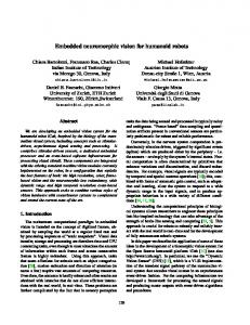
time the selected zero-crossing (enforcing the a-priori assumption that the heading direction shifts smoothly in space). An image from a typical navigation scene which shows the results of these computations is shown in Fig. 6.
Fig. 6. Image obtained from a camera mounted on a truck moving on a straight road (courtesy of B. Mathur, Rockwell Corp.) with optical flow vectors superimposed. Close to the center of the road the lane markings can be recognized, while on the left side of the image there is a shadow of a tree approaching the camera. The lower part of the image shows the 1D encoding of the horizontal component of the optical flow vectors. The vertical white bar represents the position of the heading direction as computed by the algorithm.
All the operators used in the software simulations have been implemented in the hardware architecture. Fig. 7 shows a block diagram of this architecture. The input stage is a one-dimensional array of elementary velocity sensors (described WINNER TAKE-ALL
WINNER TAKE-ALL
WINNER TAKE-ALL
WINNER TAKE-ALL
WINNER TAKE-ALL
WINNER TAKE-ALL
ZERO CROSSING
ZERO CROSSING
ZERO CROSSING
ZERO CROSSING
ZERO CROSSING
ZERO CROSSING
Vp
Vp
Vp
Vp
Vp
Vp
CURRENT SMOOTHING
CURRENT SMOOTHING
CURRENT SMOOTHING
CURRENT SMOOTHING
CURRENT SMOOTHING
CURRENT SMOOTHING
VELOCITY
VELOCITY
VELOCITY
VELOCITY
VELOCITY
VELOCITY
Fig. 7. Block diagram of the analog VLSI architecture for determining the heading direction of an observer translating in a fixed environment.
in Section II-E) that measure speed and direction of motion of temporal edges. The output voltage of each velocity sensor is then converted into current, by means of a circuit based on a two node winner-take-all (WTA) network (see Section II-D). The currents encoding the direction of motion are then spatially smoothed using two separate resistive networks (one for each direction) of the type described in Section II-C. By using a current mirror to subtract the smoothed currents from the two networks we obtain a bidirectional current, the sign of which encodes the direction of motion. Zero-crossings are detected in the third processing stage by looking for co-presence of negative currents from one unit and positive currents from the neighboring unit. The circuit that implements this operation is based on an analog current-correlator circuit [18] and on a digitally controlled current-mirror. If both input currents are greater than an externally controlled threshold value, the output is activated and a current corresponding to the sum of the absolute values of the two inputs is generated. To select the zero-crossing corresponding to the correct heading direction position we choose the one with the steepest slope (maximum current sum). This is done by feeding the output of the zero-crossing circuits to a global WTA network with lateral excitation [12]. Lateral excitation, implemented using another resistive network, accounts for the fact that the heading direction position shifts smoothly in space: it facilitates the selection of units close to the previously chosen winner and inhibits units farther away. In this way, once a strong zero-crossing is selected, the system will tend to track it as it moves along the array. Fig. 8 shows the output of the system tested on a laboratory bench. To simulate ego-motion we imaged onto the 1D array of photo-receptors (through an 8mm lens) expanding edges. This was done by placing a drawing of a V-shaped curve on a rotating drum. The 1D array would thus see sections of the V-shaped curve, starting from the bottom (edges in the center) all the way up to the top (edges in the periphery). The circuits used are non-clocked and operate in parallel, thus as soon as the photo-receptors on the chip detect moving edges, the system outputs a result. Using high-contrast, well controlled stimuli, the system is able to select and track in time the correct heading direction location.
7 6.5
6
6 5.5 5 Output Voltage
Output Voltage
5
4
3
4.5 4 3.5 3 2.5
2
2 1.5
2
4
6
8
10 12 Unit Position
14
16
18
20
22
2
4
(a)
6
8
10 12 Unit Position
14
16
18
20
22
(b)
Fig. 8. (a) Output of the system at the second processing stage (direction of velocity selection and differential voltage to current conversion) as the heading direction position shifts from left to right. The output currents were converted into voltages using an off-chip senseamplifier with a reference voltage set to 2V. Each plot was separated from the next by adding a constant value of 0.75V. (b) Output of the system at the third processing stage (zero-crossing detection) for the same sequence of heading direction positions.
IV. Conclusions We described a set of analog VLSI circuits that can be used as handy building blocks for neuromorphic vision systems. To point out how these compact circuits can be used at a system level we described a device implemented on a single 2mm × 2mm silicon chip, using 2µm CMOS technology, that is able to compute the direction of heading in the case of ego-motion in a fixed environment. We showed how these types of systems have the desirable properties of being compact, low power, low cost (if mass produced), asynchronous (non-clocked) and parallel. Nonetheless, these systems are generally characterized by low precision in their state variables and are extremely task-specific. For these reasons, we think that neuromorphic vision chips should not replace existing systems, nor try to solve autonomously complex industrial tasks. Rather, they are meant to be used in conjunction with existing engineering systems in order to simplify the pre-processing stages of the problem and to diminish the computational load of the overall system. Acknowledgments The authors would like to acknowledge the following people for making their circuits and data available and for sharing their time to explain the details of operation of several neuromorphic circuits: Tobi Delbr¨ uck, Buster Boahen, Shih-Chii Liu, Rahul Sarpeshkar, Misha Mahowald and Tim Horiuchi. This work was supported by Daimler-Benz as well as by grants from the Office of Naval Research, the Center for Neuromorphic Systems Engineering as a part of the National Science Foundation Engineering Research Center Program, and by the Office of Strategic Technology of the California Trade and Commerce Agency. Fabrication of the integrated circuits was provided by MOSIS. References [1] [2] [3]
C.A. Mead, Analog VLSI and Neural Systems, Addison-Wesley, Reading, MA, 1989. R. Douglas, M. Mahowald, and C. Mead, “Neuromorphic analogue VLSI,” Annu. Rev. Neurosci., , no. 18, pp. 255–281, 1995. T. Delbr¨ uck, “Analog VLSI phototransduction by continous-time, adaptive, logarithmic photoreceptor circuits,” Tech. Rep., California Institute of Technology, Pasadena, CA, 1994, CNS Memo No. 30. [4] K.A. Boahen and A.G. Andreou, “A contrast sensitive silicon retina with reciprocal synapses,” in Advances in neural information processing systems, D.S. Touretzky, M.C. Mozer, and M.E. Hasselmo, Eds. IEEE, 1992, vol. 4, MIT Press. [5] E.A. Vittoz and X. Arreguit, “Linear networks based on transistors,” Electronics Letters, vol. 29, no. 3, pp. 297–298, Feb. 1993. [6] J. Lazzaro, S. Ryckebusch, M.A. Mahowald, and C.A. Mead, “Winner-take-all networks of O(n) complexity,” in Advances in neural information processing systems, D.S. Touretzky, Ed., San Mateo - CA, 1989, vol. 2, pp. 703–711, Morgan Kaufmann. [7] T. Horiuchi, W. Bair, B. Bishofberger, J. Lazzaro, and C. Koch, “Computing motion using analog VLSI chips: an experimental comparison among different approaches,” International Journal of Computer Vision, vol. 8, pp. 203–216, 1992. [8] S.P. DeWeerth and T.G Morris, “Analog VLSI circuits for primitive sensory attention,” in Proc. IEEE Int. Symp. Circuits and Systems. IEEE, 1994, vol. 6, pp. 507–510. [9] G. Indiveri, J. Kramer, and C. Koch, “System implementations of analog VLSI velocity sensors,” IEEE Micro, vol. 16, no. 5, pp. 40–49, Oct. 1996. [10] A. Starzyk, J. and X. Fang, “CMOS current mode winner-take-all circuit with both excitatory and inhibitory feedback,” Electronic Letters, vol. 29, no. 10, pp. 908–910, May 1993. [11] S.P. DeWeerth and T.G Morris, “CMOS current mode winner-take-all circuit with distributed hysteresis,” Electronics Letters, vol. 31, no. 13, pp. 1051–1053, June 1995.
[12] G. Indiveri, “Winner-take-all networks with lateral excitation,” Jour. of Analog Integrated Circuits and Signal Processing, vol. 13, no. 1/2, pp. 185–193, May 1997. [13] S. Liu, “Silicon model of motion adaptation in the fly visual system,” in Proc. of Third Joint Caltech/UCSD Symposium, June 1996. [14] J. Kramer, G. Indiveri, and C. Koch, “Analog VLSI motion projects at caltech,” in Proc. Int. Symp. on Advanced Imaging and Network Technologies, Berlin, Germany, Oct. 1996. [15] J. Kramer, R. Sarpeshkar, and C. Koch, “Pulse-based analog VLSI velocity sensors,” IEEE Trans. on Circuit and Systems, vol. 44, no. 2, pp. 86–101, Feb. 1997. [16] J. Kramer, “Compact integrated motion sensor with three-pixel interaction,” IEEE Trans. Pattern Anal. Machine Intell., vol. 18, pp. 455–460, 1996. [17] E.D. Dickmanns and N. Mueller, “Scene recognition and navigation capabilities for lane changes and turns in vision-based vehicle guidance,” Control Engineering Practice, vol. 4, no. 5, pp. 589–599, May 1996. [18] T. Delbr¨ uck, ““Bump” circuits for computing similarity and dissimilarity of analog voltages,” in Proc. IJCNN, June 1991, pp. I–475–479.
Vbias
Vout
Fig. 1. Circuit diagram of the adaptive photo-receptor. The photo-diode generates a light-induced current, which is logarithmically converted into voltage and, for sharp brightness transients, amplified by a high-gain amplifier. An adaptive element in the feedback loop (the diodeconnected p-type transistor) allows the circuit to shift its optimal high-gain DC operating point with the average background brightness.
Vf Vu
Vu
Vg
Fig. 2. Circuit diagram of the current-mode outer-plexiform layer model. The photo-transistors generate light-induced current at each pixel location. The current is then diffused laterally through both excitatory and inhibitory (additive and subtractive) paths. The size and shape of the equivalent filter’s convolution kernel can be controlled by the voltages Vf and Vg .
I0 Vr
Vr
V i-1
Vr
V i+1
Vi Vg
Vg
Fig. 3. Circuit diagram of a one dimensional resistive network.
Vg
On
O n-1
I n-1
In V n-1
O n+1
I n+1 Vn
V n+1
Vg Vb Ib
Fig. 4. Circuit diagram of a winner-take-all network.
E(x-vt)
I1
I2 V
Vf1 Vs2
Vs1 V f2 Vr
Vs1 Vf2
t
Vl Vr
A
B
Fig. 5. Facilitate and sample velocity sensor. A Block diagram. Temporal-edge detectors (E) generate current pulses in response to fast image brightness transients. Pulse-shaping circuits (P) convert the current pulses into voltage signals. Voltage signals from adjacent pixels are fed into two motion circuits (M) computing velocity for opposite directions (Vl and Vr ) along one dimension. A direction-selection circuit (D) suppresses the response in the null direction to prevent temporal aliasing. B Voltage signals. The analog output voltage of the motion circuit for rightward motion (Vr ) equals the voltage of the slowly-decaying facilitation pulse (Vs1 ) at the time of arrival of the narrow sampling pulse (Vf 2 ). For leftward motion, the sampling pulse precedes the facilitation pulse and the output voltage is low. The analog output voltage thus encodes velocity for rightward motion only.
Fig. 6. Image obtained from a camera mounted on a truck moving on a straight road (courtesy of B. Mathur, Rockwell Corp.) with optical flow vectors superimposed. Close to the center of the road the lane markings can be recognized, while on the left side of the image there is a shadow of a tree approaching the camera. The lower part of the image shows the 1D encoding of the horizontal component of the optical flow vectors. The vertical white bar represents the position of the heading direction as computed by the algorithm.
WINNER TAKE-ALL
WINNER TAKE-ALL
WINNER TAKE-ALL
WINNER TAKE-ALL
WINNER TAKE-ALL
WINNER TAKE-ALL
ZERO CROSSING
ZERO CROSSING
ZERO CROSSING
ZERO CROSSING
ZERO CROSSING
ZERO CROSSING
Vp
Vp
Vp
Vp
Vp
Vp
CURRENT SMOOTHING
CURRENT SMOOTHING
CURRENT SMOOTHING
CURRENT SMOOTHING
CURRENT SMOOTHING
CURRENT SMOOTHING
VELOCITY
VELOCITY
VELOCITY
VELOCITY
VELOCITY
VELOCITY
Fig. 7. Block diagram of the analog VLSI architecture for determining the heading direction of an observer translating in a fixed environment.
7
6
Output Voltage
5
4
3
2
2
4
6
8
10 12 Unit Position
14
16
18
20
22
16
18
20
22
(a)
6.5 6 5.5
Output Voltage
5 4.5 4 3.5 3 2.5 2 1.5 2
4
6
8
10 12 Unit Position
14
(b) Fig. 8. (a) Output of the system at the second processing stage (direction of velocity selection and differential voltage to current conversion) as the heading direction position shifts from left to right. The output currents were converted into voltages using an off-chip senseamplifier with a reference voltage set to 2V. Each plot was separated from the next by adding a constant value of 0.75V. (b) Output of the system at the third processing stage (zero-crossing detection) for the same sequence of heading direction positions.