New Composite Operations and Precomputation Scheme for Elliptic Curve Cryptosystems over Prime Fields (Full version) Patrick Longa1, and Ali Miri2 Department of Electrical and Computer Engineering University of Waterloo, Canada
[email protected] 2 School of Information Technology and Engineering (SITE) University of Ottawa, Canada
[email protected] 1
Abstract. We present a new methodology to derive faster composite operations of the form dP+Q, where d is a small integer ≥ 2, for generic ECC scalar multiplications over prime fields. In particular, we present an efficient DoublingAddition (DA) operation that can be exploited to accelerate most scalar multiplication methods, including multiscalar variants. We also present a new precomputation scheme useful for window-based scalar multiplications that is shown to achieve the lowest cost among all known methods using only one inversion. In comparison to the remaining approaches that use none or several inversions, our scheme offers higher performance for most common I/M ratios. By combining the benefits of our precomputation scheme and the new DA operation, we can save up to 6.2% in the scalar multiplication using fractional wNAF. Keywords: Elliptic curve cryptosystem, scalar multiplication, point operation, composite operation, precomputation scheme.
1 Introduction Elliptic curve cryptography (ECC) was independently introduced by Koblitz and Miller in 1985. Since then, this public-key cryptosystem has attracted increasing attention due to its shorter key size requirement in comparison with other established systems such as RSA and DL-based cryptosystems. For instance, it is widely accepted that 160-bit ECC offers equivalent security to 1024-bit RSA. This significant difference makes ECC especially attractive for applications in constrained environments as shorter key sizes are translated to less power and storage requirements, and reduced computing times. Scalar multiplication, denoted by kP, where k is the secret key (scalar) and P is a point
This manuscript is also available at http://patricklonga.bravehost.com/publications.html The short version of this paper will appear in the Proceedings of the 11th International Workshop on Practice and Theory in Public Key Cryptography (PKC 2008), Lecture Notes in Computer Science (LNCS), Vol. 4939, Springer.
2
P. Longa and A. Miri
on the elliptic curve, is the central operation of elliptic curve cryptosystems. Methods to efficiently compute such operation have traditionally exploited the binary expansion of numbers (e.g., NAF and wNAF). This is mainly due to the fact that the binary expansion directly translates to computations using the simplest elementary ECC point operations, namely point doubling and addition. However, recent developments in the field suggest that it is possible to use more complex operations to accelerate the scalar multiplication [4,7,8,24]. For instance, Ciet et al. [4] introduced the ternary/binary method using radices 2 and 3 for the representation of the scalar. Dimitrov et al. [7] proposed the double-base number system for the scalar multiplication using mixed powers of 2 and 3. Radix 5 was added to the previous approach by Mishra et al. [21] to represent scalars with mixed powers of 2, 3 and 5. More recently, Longa and Miri [18] have proposed the multibase non-adjacent form (mbNAF) method, which uses a very efficient representation of integers using multiple bases. Efficiency of the previous methods strongly depends on the costs of such operations as tripling (3P, denoted by T) or quintupling (5P, denoted by Q) of a point, unified doublingaddition (2P+Q, denoted by DA), unified tripling-addition (3P+Q, denoted by TA), unified quintupling-addition (5P+Q, denoted by QA), among others. Thus, it is a critical task to reduce the computing cost of these operations, which are referred to as composite operations since they are inherently based on basic doubling and addition, to further speed up the execution time of the scalar multiplication. In the first part, we propose a new technique to derive faster composite operations of the form dP+Q, where d is a small integer ≥ 2 and P, Q are points on the elliptic curve in Jacobian and affine coordinates, respectively. As pointed out, operations of this form are highly common in all known scalar multiplication methods, including multiscalar versions which are used in the ECDSA signature verification [12]. For instance, DA is a recurrent operation in NAF, wNAF and Shamir’s trick, where each mixed Jacobian-affine addition is always computed right after a doubling. In addition to DA, TA is used in the doublebase method [7], and TA and QA in the triple-base [21] and mbNAF methods [16,18]. Our technique makes use of Meloni’s idea of adding two points with the same z coordinates [19] (which we will refer to as special addition with identical z-coordinate) to have an iterative computation of the form dP+Q = P+…+P+(P+Q), which is computed backwards and where only the first addition shown in parentheses is computed with a traditional mixed addition. Every extra addition can then be efficiently computed with the addition with identical z-coordinate. We show that our new composite operations are more efficient than formulas using the cheapest operations existent in current literature. See [17] for the state-of-the-art point formulas in Jacobian coordinates. In the second part, we modify the previous methodology to yield a new scheme for the precomputation of points in window-based methods such as wNAF and fractional wNAF (denoted by Frac-wNAF). Using pre-stored points is a practical technique to accelerate the scalar multiplication when there is extra memory available. However, for scalar multiplications kP with P unknown, the precomputation of such points is necessarily done on-line and its time execution included in the whole time estimation of the scalar multiplication. Examples of this case can be found during decryption in the ElGamal
New Composite Operations and Precomputation Scheme
3
encryption scheme or in the Diffie-Hellman key exchange. Thus, it is crucial to reduce the time for the precomputation to boost the savings achieved by window-based methods. Given that precomputations follow the form diP, where di are the odd integers in the range [3, m] with m ≥ 3, we modify our original approach to the iterative computation of the form diP = 2P+…+2P+2P+P, which is again computed backwards, and requires one point doubling followed by cheaper additions with identical z-coordinate. Following, and to keep advantage of the efficient mixed addition during the scalar multiplication, points are converted to affine representation using the well-known Montgomery’s method which permits to reduce the number of expensive inversions to only one. Moreover, this method is further sped up by efficiently using values computed during the first stage of our methodology. For the latter, two variants with different memory requirements are presented, which will be shown to be suitable for different window widths. Our precomputation scheme is compared with the best previous approaches using only one inversion, and shown to deliver the lowest cost. In comparison to methods using none or several inversions, our scheme is shown to offer the highest performance for most common I/M ratios. Our work is organized as follows. In Section 2, we detail some background about ECC over prime fields. Then, we present our methodology based on the special addition with identical z-coordinate, and apply it to derive efficient composite operations of the form dP+Q, whose costs are compared to previous formulae right after. In Section 4, a variant of the previous methodology is used to build a new precomputation scheme for windowbased scalar multiplications. The cost and memory requirements of our scheme are then discussed and compared with previous efforts. Some conclusions summarizing the contributions of this work are presented at the end.
2 Preliminaries An elliptic curve E over a prime field p (denoted by E ( p ) ) is defined by the reduced Weierstrass equation [12]:
E : y x ax b . 2
3
(1)
Where: a , b p and 4a + 27b 0 . The set of pairs ( x, y ) that solves (1), where x, y p , and the point at infinity , which is the identify for the group law, form an abelian group ( E ( p ) ,+), on top of which the ECC computations are performed. The main operation in ECC is known as scalar multiplication, which is denoted by Q kP, where P and Q are points in E ( p ) , and k is the secret scalar. The simplest representation of points on the elliptic curve E with two coordinates ( x, y ) , namely affine coordinates (denoted by ), introduces field inversions into the computation of point doubling and addition. Inversions over prime fields are the most expensive field operation and are avoided as much as possible. Although their relative cost depends on the characteristics of a particular implementation, it has been observed 3
2
4
P. Longa and A. Miri
that, especially in the case of efficient forms for the prime p as recommended by [11], the inversion can result as computationally expensive as 1I > 30M. For instance, benchmarks presented by [15] and [2,12] show I/M ratios between 30-40 and 50-100, respectively. Projective coordinates (X, Y, Z) solve the previous problem by adding the third coordinate Z to replace inversions with a few other field operations. The foundation of these inversion-free coordinate systems can be explained by the concept of equivalence class, which is defined in the following in the context of Jacobian coordinates (), a special case of projective coordinates that has yielded very efficient point formulae [10]. Given a prime field p , there is an equivalence relation among non-zero triplets over p , such that [1]:
( X 1 , Y1 , Z1 ) ( X 2 , Y2 , Z 2 ) X 1 2 X 2 , Y1 3Y2 and Z1 Z 2 , for some p* . Thus, the equivalence class of a (Jacobian) projective point, denoted by (X : Y : Z), is:
(X : Y : Z) {( 2 X, 3Y, Z) : p*} .
(2)
It is important to remark that any (X, Y, Z) in the equivalence class (2) can be used as a representative of a given projective (Jacobian) point. In the following, we succinctly summarize costs of the improved formulae in introduced by [17], which applied an effective technique to speed up the traditional point operations. The improved formulae will be later used for comparison with our new composite operations in Section 3. For further details about point formulae the reader is referred to [17]. Also, to ease the work of implementers, we keep a record of the most efficient point formulas in at: http://patricklonga.bravehost.com/jacobian.html. The cost of using the Jacobian representation for the doubling formula has been found to be 2M + 8S (reduced from the traditional 4M + 6S). When w successive executions of several doublings are used, the cost is (3w)M + (5w + 2)S by combining our strategy in [17] to accelerate operations with the approach by [14], which means that doublings are performed with only 3M + 5S, with exception of the first one that costs 3M + 7S. Also, it is important to note that it has been suggested that the parameter a (see (1)) be fixed at 3 for efficiency purposes. In fact, most curves recommended by public-key standards [13] use a 3, which has been shown to not impose significant restrictions to the cryptosystem [3]. In this case, the cost of point doubling is reduced to only 3M + 5S. In the remainder of this work, we will refer to the special case when a 3, and the general case when the parameter is not fixed and can be any value in the field. In the case of addition, representing one of the points in and the other in has yielded the most efficient addition formula, which is known as mixed Jacobian-affine addition and presents a cost of 8M + 3S [5]. In [17], the cost of this operation was reduced further to only 7M + 4S. If one considers both points to be added in , then the cost is 12M + 4S (reduced to 11M + 5S by [17]). We will refer to the latter as general addition in .
New Composite Operations and Precomputation Scheme
5
In the case of the tripling, Longa and Miri improved the formula proposed by [7] and reduced its cost from 10M + 6S to 6M + 10S in the general case, and to only 7M + 7S if one fixes a 3 [17]. Similarly, an efficient quintupling was presented by the same authors [18] with costs of 10M + 14S in the general case and only 11M + 11S when a 3 , improving the formulae by [21] that cost 15M + 10S and 15M + 8S for the corresponding cases. Variants of have also been proposed. In particular, the four-tuple (X, Y, Z, aZ 4) and m five-tuple (X, Y, Z, Z 2, Z 3) , known as modified Jacobian ( ) and Chudnovsky () coordinates, respectively, permit to save some operations by passing recurrent values between point operations. Also, a technique that combines different representations (known as mixed coordinates) to yield efficient schemes for the scalar multiplication including precomputation was presented by [5]. We discuss the application of these mixed representations in Section 4. The reader is referred to [1,5] for further details.
3 Composite Operations dP + Q Our strategy to yield cheaper composite operations of the form dP+Q is based on the efficient use of the new addition formula with identical z-coordinate introduced by Meloni [19], which is described in the following. Let P ( X 1 , Y1 , Z ) and Q ( X 2 , Y2 , Z ) be two points with the same z coordinates in on the elliptic curve E. The addition P Q ( X 3 , Y3 , Z 3 ) can be obtained as follows:
X 3 Y2 Y1 X 2 X 1 2 X 1 X 2 X 1 . 2
3
2
Y3 Y2 Y1 X 1 X 2 X 1 X 3 Y1 X 2 X 1 .
Z3 Z X 2 X 1 .
2
3
(3)
This new addition only costs 5M + 2S, which represents a significant reduction in comparison with 7M + 4S corresponding to the mixed Jacobian-affine addition. Sadly, it is not possible to directly replace traditional additions with this special operation since, obviously, it is expected that additions are computed over operands with different z coordinates during the scalar multiplication. The author in [19] applied his formula to the context of scalar multiplication with star addition chains, where the particular sequence of operations allows the replacement of each traditional addition by (3). However, we noticed that the new addition can in fact be applied to a wider context with traditional scalar multiplication methods. In the following, we develop faster composite operations by exploiting the advantages of this special addition on ECC using generic scalar multiplications over prime fields.
6
P. Longa and A. Miri
3.1
Our Methodology
We propose to compute dP + Q as follows: dP + Q = P +… + P + P + (P+Q) ,
(4)
where d is a small integer ≥ 2, and P, Q are points in and on E ( p ) , respectively. Strategy (4) would lead to high costs if computed with mixed and general additions. However, we will show in the following that only the first addition in parentheses needs to be computed with a mixed addition. Then, every extra addition can be computed with (3). First, we compute P Q ( X 1 , Y1 , Z1 ) ( X 2 , Y2 ) ( X 3 , Y3 , Z 3 ) as mixed Jacobianaffine addition with the following [17]:
X 3 4 Z1 Y2 Y1 4 Z1 X 2 X 1 8 X 1 Z1 X 2 X 1 . 2
3
3
2
2
2
Y3 2 Z1 Y2 Y1 4 X 1 Z1 X 2 X 1 X 3 8Y1 Z1 X 2 X 1 . 3
2
2
Z 3 2 Z1 Z 1 X 2 X 1 Z 1 Z 1 X 2 X 1 2
2
2
3
2
Z1 Z 1 X 2 X 1 . 2
2
2
(5)
The main observation from (5) is that if we assume the next new representation for P:
X
(1) 1
(1)
4 X Z
(1)
, Y1 , Z1
1
X 2 X1
2 1
2
, 8Y1 Z1 X 2 X 1 2
3
, 2 Z1 Z1 X 2 X 1 2
X , Y , Z , (6) 1
1
1
we can use the special addition (3) to perform the next addition between P and (P+Q) because both points would have the same z coordinate. It is important to note that the 2 equivalence relation in (6) holds by fixing Z1 X 2 X 1 in the equivalence class for given in (2). Most importantly, the equivalent point X 1(1) ,Y1(1) , Z1(1) does not require any extra computation because its coordinates have already been computed in (5). Similarly, every extra addition with P according to (4) can be performed with the special addition (3) as P always has an equivalent point with the same z coordinate as the resultant point of the previous computation. In fact, we observe that every addition outside the parentheses in (4) adjusts to the next generic formulae for j 1 to ( d 1) :
j
j
j
P P P ( P Q ) X 1 , Y1 , Z1 ( j 1) terms
X j 3 Y j 2 Y1
Y j 3 Y j 2 Y1 j
Z j 3 Z1
X
j
X X X X , 2
j
j
j
1 j
j2
j
j
X1
j2
3
j
j2
X1
j
2 X1
2
X X
j2
, Yj 2 , Z j 2 X j 3 , Yj 3 , Z j 3 : j
j2
X j 3 Y1
X1 j
X
2
, j
j2
X1
, 3
(7)
1
j
where X 1 , Y1 , Z1 denotes the equivalent point to P for the jth addition. As we can see in (7) it holds that one always gets an equivalent point to P for the following addition by fixing:
X
j 1 1
, Y1
j 1
j 1
, Z1
X X j
1
j
j 2
X1
2
, Y1
j
X
j
j2
X1
3
j
, Z1
X
j
j 2
X1
,
New Composite Operations and Precomputation Scheme
j
j
j
7
which is equivalent to X 1 , Y1 , Z1 according (2), and has the same z coordinate as (7). The cost of (4) is given by 1A + (d 1)A’, where d , d ≥ 2, A and A’ denote the cost of the mixed and special additions, respectively. Thus, strategy (4) would cost (7M + 4S) + (d 1) (5M + 2S). However, in the following section we will show that by merging the mixed addition between parentheses (see (4)) with the first special addition it is possible to achieve additional savings. Unified Doubling-Addition (DA) Operation When d = 2, the strategy (4) can be used to perform a doubling-addition (DA) operation as P + (P+Q). We can reduce further the cost of this operation by unifying the first two point additions (i.e., mixed and special additions) into the following unified DA formulae:
X 4 2 X 1 , Y4 X 1 X 4 Y1 , Z 4 Z1 . 2
Where:
3
(1)
2
(1)
2
(1)
3
(1)
(8)
Z1 Y2 Y1 , Z1 X 2 X 1 , 3
2
X 1 4 X 1 , Y1 (1)
2
(1)
8Y1 , Z1 Z1 Z1 , 3
2
(1)
2
2
X 3 X 1 4[ 3 X 1 ] , (1)
Y3 Y1
(1)
2
3
2
16Y1 . 2
2
2
3
Note that we directly compute X 3 X 1 and Y3 Y1 to avoid the intermediate computations of X3, Y3 and Z3 from the first addition (5), saving some field additions and trading one multiplication for one squaring. Thus, the cost of the unified DA is fixed at only (6M + 5S) + (5M + 2S) = 11M+7S. Based on this formula, we can now define the total cost of our methodology for computing composite operations of the form dP+Q. Using (8) to perform the mixed addition and the first special addition, the methodology (4) costs: (6M + 5S) + (d 1) (5M + 2S), (9) (1)
(1)
where d 2 for a composite operation of the form dP+Q. Note that, after executing the DA operation as P + (P+Q), the procedure described in Section 3.1 still applies. Hence, the cost of a special addition (i.e., 5M + 2S) is added at every extra addition with P in (4). Let us now compare the cost of the methodology (4) with previous formulae. For instance, when d = 2, (4) computes the DA operation with a cost of 11M + 7S, which is superior to the traditional execution consisting of a doubling followed by a mixed addition: 12M + 7S if a 3 . In this case, the proposed DA reduces the cost in one multiplication. The new operation is even superior to the improved formulas by [17]: (3M + 5S) + (7M + 4S) = 10M + 9S, trading one multiplication for two squarings.
8
P. Longa and A. Miri
Remarkably, because our strategy does not involve a traditional doubling, the same aforementioned cost for DA is achieved when the parameter a in (1) is randomly chosen. In contrast, a general doubling followed by a mixed addition costs 12M + 9S, or (2M + 8S) + (7M + 4S) = 9M + 12S with the formulas by [17]. In this case, the new DA reduces the cost in one multiplication and two squarings (or trades two multiplications for five squarings, in the second case). We remark that 2P+Q is a recurrent operation in efficient scalar multiplications. Thus, the new DA can be used to speed up well-known methods such as NAF, wNAF and the Shamir’s trick [12] by directly replacing every doubling followed by a mixed addition. Also, it is important to remark that, as expected, adding one point P at a time in the methodology (4) results efficient for small values of d, specifically when d = 2 and 3. For higher values of d it is better to take advantage of the already efficient doubling, tripling and quintupling operations. In this case, we propose to first perform some computation on the point P using these operations and then apply our approach to the result. For instance, for d = 4, 6, 7 and 8, dP+Q would be computed as follows: 3.2
4P+Q = 2P + (2P+Q), which involves a point doubling followed by a DA. 6P+Q = 3P + (3P+Q), which involves a point tripling followed by a DA. 7P+Q = P + (3P + (3P+Q)), which involves a point tripling followed by DA and a general addition. 8P+Q = 4P + (4P+Q), which involves two point doublings followed by DA. Performance Comparison
Cost estimates using our strategy (4) and the traditional formulae for different composite operations of the form dP+Q are summarized in Table 1. Since we could not find in the literature any effort to accelerate composite operations of the form dP+Q in the case of projective (Jacobian) coordinates over prime fields, new composite operations are compared against operations combining the fastest point operations of form dP (i.e., improved doubling, tripling and quintupling by [17,18]) with addition, in the most efficient way. Thus, 2P+Q, 3P+Q and 5Q+P are computed by a doubling, tripling and quintupling, respectively, followed by a mixed addition; 4P+Q and 8P+Q, by two and three consecutive doublings, respectively, and a mixed addition; 6P+Q, by one doubling, one tripling and one mixed addition; and 7P+Q, by three doublings, one general addition (with –P) and one mixed addition. Note that approaches in Table 1 have been slightly improved for the general case by saving some operations during computation of consecutive doublings (d = 4, 8), as detailed in Section 2. Also, for the general case, d = 6, we have reduced the cost further by saving two squarings during computation of a doubling followed by a tripling (see details in Appendix A). In the case of the proposed composite operations, we show performance when applying the methodology (4) in cases d = 2, 3 and 5, whose cost is given by (9). For d
New Composite Operations and Precomputation Scheme
9
4, 6, 7 and 8, we use the already efficient DA in combination with the fast doubling, tripling or quintupling by [17,18], as described in Section 3.1. Table 1. Performance of proposed composite operations of the form dP+Q in comparison with previous formulae. Method
2P+Q
3P+Q
4P+Q
5P+Q (a)
14M + 12S 13M + 15S
6P+Q
7P+Q (a,b)
18M +14S 29M + 19S 17M + 17S (b) 28M + 22S
Ours (5)
11M + 7S
Previous [17,18]
10M + 9S (a) 14M + 11S (a,b) 13M + 14S (a) 18M + 15S (a,c) 17M +16S (a) 9M + 12S 13M + 14S (b) 13M + 16S 17M + 18S (c) 16M + 19S
16M + 9S
26M + 13S
8P+Q (a)
17M + 17S (a) 16M + 20S
28M + 21S (a) 16M + 19S (a) 27M + 24S 16M + 21S
(a) Parameter a is fixed to3, (b) Using tripling by [17], (c) Using quintupling by [18].
As we can see, our methodology reduces costs in comparison with the best implementations using previous operation formulae. The only exception is when d = 3 (special case) or 5, where the efficient tripling and quintupling formulas previously presented in [17] and [18], respectively, permit to achieve the lowest costs. In the most frequent scenario, our new composite operations introduce some savings by trading one multiplication for two squarings (special case, d = 2, 4, 8; both cases, d = 6, 7). In other cases, we trade up to five squarings for only two multiplications (general case, d = 2), or save one squaring (general case, d = 4, 8). The reader must note that the savings are more dramatic if we compare the presented cases with the traditional formulae [12] or the composite operations by [7,21].
4 New Method for Precomputation Precomputed points are extensively used to accelerate the scalar multiplication in applications where extra memory is available. Well-known methods in this category are wNAF and Frac-wNAF, which rely on precomputations to reduce the Hamming weight of the binary expansion of the scalar, and thus, reduce the cost of the scalar multiplication. In particular, Frac-wNAF requires building the following table with digits di [22]:
d i Di 1, 3, 5,..., m .
(10)
Using the digit set (10), the average non-zero density for Frac-wNAF is [22]:
log 2 m
( m 1) 2
log 2 m
1
1
.
(11)
It is important to remark that Frac-wNAF is a generalization of wNAF and covers all the possibilities in terms of memory requirements. We propose a variation to strategy (4) and compute the precomputed table as follows:
10
P. Longa and A. Miri
diP = … + 2P + 2P + 2P + P .
(12)
We will show that all the additions in (12) can be computed with the special addition with identical z-coordinate (3), reducing costs in comparison with previous approaches. Further, some values computed during the mentioned additions are efficiently exploited to minimize costs. In this regard, we present two schemes with different memory requirements that achieve high performance. For the remainder of this work, we refer to them as Schemes 1 and 2. Our method can be summarized in the following two steps. Step 1: Computation of precomputed points in Jacobian coordinates Point P is assumed to be originally in . Thus, if we want to use the special addition, we should translate computations to . By applying the mixed coordinates approach proposed in [5], we can compute the doubling 2P in (12) in and yield the result in as follows:
X 2 3x12 a 2 , Y2 3x12 a X 2 8y14 , Z 2 2y1 . 2 With: 4x1 y12 2 x1 y12 x12 y14 , 2
(13)
where the input and result are P (x1 , y1) and 2P (X 2 , Y2, Z 2) , respectively. Formula (13) is easily derived from the doubling formula in [12] by applying (2) with 2y1 , and has a cost of only 1M + 5S. Note that we have reduced the cost of (13) by replacing the multiplication 4x1 y12 by one squaring and other cheaper operations. Then, by fixing 2 y1 in (2) we can assume the following equivalent point to P:
P (1) X 1(1) , Y1(1) , Z1(1) 4 x1 y12 , 8 y14 , 2 y1 X 1 , Y1 , Z1 ,
(14)
which does not introduce extra costs since its coordinates have already been computed in (13). Following additions to compute digits di would be performed using (4) as follows: 3P 2 P P
1st
Y
1
Z3 Z2
X
X Y X X X X . (1)
X 3 Y1 Y3
(1)
Y2
2
2
(1)
2
2
(1)
(1 )
(1)
2X X X X X Y X 3
X2
1
(1 )
, Y2 , Z 2 X 1 , Y1 , Z 1
(1) 1
3
1
2
(1)
2
3
2
3
3
:
2
(1)
2
2
X ,Y , Z . X .
1
3
2
(1)
1
2
X X X , Y X X , Z X 5P 2 P 3P X , Y , Z X , Y , Z X , Y , Z : X Y Y X X 2 X X X . Y Y Y X X X X Y X X .
2nd Having 2 P
(1)
X , Y , Z (1)
(1 )
2
(1)
(1 )
2
(1)
4
3
4
3
2
(1)
(1)
3
2
3
3
2
(1)
3
2
1
3
4
(1)
3
2
2
1
4
(1 )
3
2
2
4
2
2
(1 )
4
2
3
3
(1)
2
(1)
2
(1)
2
(1 )
2
2
(1)
2
(1 )
2
2
2
(1)
2
3
2
(1 ) 1
X2
X
2
, Y2 , Z 2
,
New Composite Operations and Precomputation Scheme (1)
Z4 Z2
X
(1)
3
X2
, A X X 4
3
(( m 1) / 2)
th
Having 2 P , Y2
mP 2 P
(( m 3 ) / 2 )
mP 2 P
(( m 3 ) / 2 )
(( m 5 ) / 2 )
Y( m 3 ) / 2 Y( m 1 ) / 2 Y2 (( m 3 ) / 2 )
( m 1) / 2
( m 2) P
Z ( m3) / 2 Z 2
X
(( m 3 ) / 2 )
(( m 3 ) / 2 )
X
X
X
X
(( m 3 ) / 2 ) 2
X2
(( m 3 ) / 2 ) 2
( m3) / 2
X
, Y2
X
B4
, Y2
(( m 3 ) / 2 )
,Z 3
2
X , X
3
(( m 3 ) / 2 )
X2
, C X X
2
4
X
3
( m 1) / 2
X2
X
X X
(1) 2
.
(( m 5 ) / 2 ) 2
(( m 5 ) / 2 )
(( m 3 ) / 2 )
X2
( m 1) / 2
2
X
, Z2
(( m 3 ) / 2 )
( m 1) / 2
(( m 3 ) / 2 )
(( m 3 ) / 2 )
(( m 5 ) / 2 )
(( m 3 ) / 2 )
(1)
X2
3
, Z2
, Y( m 3 ) / 2 , Z ( m 3 ) / 2
2
X
(( m 5 ) / 2 )
( m 1 ) / 2
(( m 5 ) / 2 )
2
, Y( m 1) / 2 , Z ( m 1 ) / 2
( m 1 ) / 2
3
X2 ,Y2
(( m 5 ) / 2 )
2
,
(( m 5 ) / 2 )
,Z2
,
: (( m 3 ) / 2 )
2X2
X 2
( m 3) / 2
X
Y
(( m 3 ) / 2 )
( m 1) / 2
(( m 3 ) / 2 )
2
X2
X
2
,
(( m 3 ) / 2 )
( m 1) / 2
X2
, 3
(( m 3 ) / 2 )
( m 1) / 2
(( m 3 ) / 2 )
A( m 3 ) / 2 X ( m 1) / 2 X 2
(( m 5 ) / 2 )
( m 2) P
X ( m 3 ) / 2 Y( m 1) / 2 Y2
(( m 3 ) / 2 )
,
(1) 2
11
X2
, B
( m3) / 2
(( m 3 ) / 2 )
( m 1) / 2
X2
2
,C
( m3) / 2
(( m 3 ) / 2 )
X ( m 1) / 2 X 2
. 3
Values Ai and (Bi, Ci), for i = 4 to (m+3)/2, are stored for Schemes 1 and 2, respectively, and used in Step 2 to save some computations when converting points to . Step 2: Conversion to affine coordinates Points X i , Yi , Z i from Step 1, for i from 3 to (m+3)/2, have to be converted back to since this would allow the use of the efficient mixed addition during the scalar multiplication. This can be achieved by means of the following:
(X i / Z i2, Yi / Z i3, 1) .
(15)
To avoid the computation of several expensive inversions when using (15) for each point in the case m 3 (10), we use the method due to Montgomery, called simultaneous inversion [12], to limit the requirement to only one inversion. 1 In Scheme 1, we first compute the inverse r Z ( m 3) / 2 , and then recover every point using (15) as follows: mP :
x( m 3) / 2 r X ( m 3) / 2 , y( m 3) / 2 r Y( m 3) / 2 . 2
3
(m2)P : r r A( m 3) / 2 , x( m 1) / 2 r X ( m 1) / 2 , y( m 1) / 2 r Y( m 1) / 2 . 2
3
3P :
r r A4 , x3 r X 3 , y3 r Y3 . 2
3
j
It is important to observe that Z j Z 3
A , for j 4 to (m3)/2, according to Step 1, i
i 4
12
P. Longa and A. Miri 1
and hence, for i (m2) down to 3, Z ( i 3) / 2 for each point iP is recovered at every multiplication r A( i 5 ) / 2 . 2 3 1 1 For Scheme 2, we first compute r1 Z ( m 3) / 2 and r2 Z ( m 3) / 2 , and then recover every point using (15) as follows:
mP :
x( m 3) / 2 r1 X ( m 3) / 2 , y( m 3) / 2 r2 Y( m 3) / 2 .
(m2)P : r1 r1 B( m 3) / 2 , r2 r2 C ( m 3) / 2 , x( m 1) / 2 r1 X ( m 1) / 2 , y( m 1) / 2 r2 Y( m 1) / 2 .
3P :
r1 r1 B4 , r2 r2 C4 , x3 r1 X 3 , y3 r2 Y3 . j
2
2
In this case: Z j Z 3
B
i
i4
j
3
3
and Z j Z 3
C i4
i
, for j 4 to (m3)/2 , according to 2
3
Step 1, and hence, for i (m2) down to 3, the pair ( Z ( i 3) / 2 , Z ( i 3) / 2 ) for each point iP is recovered with r1 B( i 5) / 2 and r2 C( i 5 ) / 2 . The reader is referred to Appendix B for the pseudocodes of Schemes 1 and 2. 4.1
Cost Analysis
In total, Scheme 1 has the following cost when computing the precomputed table (10):
Cost Scheme 1 1I (9 L ) M (3 L 5) S ,
(16)
where L ( m 1)/2 represents the number of points. In terms of memory usage, Scheme 1 requires (3L+) registers for temporary calculations and storing the precomputed points. We will show later that this requirement does not exceed the number of available registers for the scalar multiplication for practical values of L. In the case of Scheme 2, the cost is as follows:
Cost Scheme 2 1I (9 L ) M (2 L 6) S ,
(17)
For this scheme, we require (4L+1) registers when L > 1. For L = 1, the requirement is fixed at 6 registers. It will be shown that this requirement does not exceed the memory allocated for scalar multiplication for small values of L. For a detailed description of the estimation of costs and memory requirements for Schemes 1/2, we refer to Appendix C. As we can see from (16) and (17), Scheme 2 reduces further the cost to compute the precomputed table at the expense of some extra memory. In the following, we analyze the memory requirements for the scalar multiplication and determine if our method adjusts to such constrains. Considering that the precomputed table requires 2L registers for storing L points, the total requirement of the scalar multiplication is given by (2L+R) registers, where R is the number of registers needed by the most memory-consuming point operation in a given implementation. On scalar multiplications using solely radix 2, addition is usually such
New Composite Operations and Precomputation Scheme
13
operation. Depending on the used coordinates and/or implementation details, point m addition can require from 7/8 registers in [12] and , respectively, to 8 registers for an SSCA-protected version [20]. If the scalar multiplication includes radix 3 in its expansion, then tripling becomes the most expensive operation with a requirement of up to 9/10 registers [7,17]. Consequently, Scheme 2 adjusts to the previous requirements for small precomputed tables with L = 1 to 3 if addition is the main operation. If we also consider tripling, Scheme 2 is suitable for values L = 1 to 4. In the case of Scheme 1, it follows the memory constrains for values L = 1 to 5 and L = 1 to 7 for radix-2 and radix-3 cases, respectively, which demonstrates that this scheme is efficient for practical FracwNAF implementations. The reader must note that, in general, values L 7 are not efficient since the cost of computing the precomputed table results more expensive than the savings achieved by precomputation during the scalar multiplication. In the following section, we analyze the performance of our method in comparison with previous efforts. 4.2
Performance Comparison
There are different efficient schemes to compute precomputed points in the literature. The simplest approaches suggest performing computations in or using the chain P → 3P → 5P → … → mP. The latter requires one doubling and L ( m 1)/2 additions, which can be expressed as follows in terms of field operations for the mentioned cases:
Cost ( L 1) I (2 L 2) M ( L 2) S . Cost (10 L 1) M (4 L 5) S .
(18) (19)
Note that (19) shows a better performance than the estimated cost given by [6] since we are considering that the doubling 2P is computed as 2 → with a cost of 2M + 5S, the first addition P + 2P computed with a mixed addition as + → (7M + 4S), and the following (L1) additions as + → (10M + 4S). The new operation costs are obtained by applying the technique of replacing multiplications by squarings introduced in [17]. The memory requirements of the - and -based methods are 2L+R and 5L+R registers, respectively. Other methods that achieve better performance in scenarios where inversion is relatively expensive, perform computations in Projective (), or coordinates and, then, convert the points to by using the Montgomery’s method to reduce the number of required inversions to only one. Cost for these methods are shown in the following [6,9], considering the general assumption 1S 0.8M:
Cost 1I (16 L 3) M (3 L 5) S 1I (18.4 L 1) M . Cost 1I (16 L 5) M (5 L 5) S 1I (20 L 1) M . Cost 1I (16 L 4) M (5 L 5) S 1I (20 L ) M .
(20) (21) (22)
14
P. Longa and A. Miri
Recently, Dahmen et al. [6] proposed a new scheme, whose computations were efficiently performed using solely formulae in . Also, the number of inversions was limited to only one by means on the Montgomery’s method. This scheme costs:
Cost [6] 1I (10 L 1) M (4 L 4) S 1I (13.2 L 2.2) M ,
(23)
that shows its superiority when compared with all the previous methods requiring only one inversion. However, our method achieves even lower costs as shown in Section 4.1:
Cost Scheme 1 1I (11.4 L 4) M , Cost Scheme 2 1I (10.6 L 4.8) M . which make our approach, and specifically Scheme 2, the fastest in the literature when the number of inversions is limited to one. For comparing with the approach (18), which includes several field inversions in their computation, it is better to specify the range of I/M ratios for which each method is superior. Table 2 shows the I/M values for which our schemes and the -based scheme are the most efficient for a given number of precomputed points. To present a fair comparison, methods are compared according to the memory constrains for the scalar multiplication using radix-2. As analyzed in Section 4.1, Schemes 1 and 2 are suitable for values L = 1 to 5 and L = 1 to 4, respectively. Table 2. I/M ranges for which each method achieves the lowest cost. # Points Scheme 1 Scheme 2 Affine (18)
1
2
3
4
5
≥9
≥ 8.4
≥ 8.2
≥ 8.1
≥ 8.7
≤9
≤ 8.4
≤ 8.2
≤ 8.1
≤ 8.7
As it can be seen, our schemes outperform the -based approach for the most commonly found I/M ratios, where inversion is relatively expensive. In average, Schemes 1 and 2 are superior when inversion is more than 9 times the cost of multiplication. As discussed in Section 2, it is usually expected that I/M 30. Finally, we compare performance of our schemes with the -based approach, whose cost is given by (19). In this case, we should also consider the scalar multiplication cost in our comparisons since precomputations in require different computing and memory requirements to the case. When precomputations are in , [5] proposed the use of + m m → to perform additions (10M + 6S), 2 → to every doubling preceding an m m addition (2M + 5S), and 2 → (3M + 5S) to the rest of doublings. Note that we have reduced further the cost of the mentioned operations by applying the same technique introduced in [17] to replace multiplications by squarings. Following this scheme, the scalar multiplication cost including precomputations is as follows:
New Composite Operations and Precomputation Scheme
15
n ((10 M 6 S ) (2 M 5 S )) n(1 )(3M 5S ) (10 L 1) M (4 L 5) S ,
(24)
where represents the Hamming weight as expressed in (11). For our approach, we consider an improved scheme taking advantage of the faster DA operation proposed in Section 3.1. Thus, we use + (+) → to perform doublingaddition operations following the form P + (P+Q) with a cost of 11M + 7S, and the fast point operations by [17]. With this scheme, the scalar multiplication cost including precomputations is as follows:
n (11M 7 S ) n(1 )(3M 5S ) Cost
Scheme 1 / 2
.
(25)
We also include in our comparison a traditional scheme using and only one inversion to assess the advantages of our improved scheme (25). By using (21) and the point operations by [17], the cost of the scalar multiplication including precomputations is given by:
n (7 M 4 S ) n(3M 5S ) 1I (20 L 1) M ,
(26)
Figure 1. Cost performance of the proposed scheme and previous methods to perform the scalar multiplication including precomputation (1I = 30M, 1S= 0.8M, n 160 bits).
J-based
Field Multiplications (M)
1750
C-based Proposed
1700 1650 1600 1550 1500
1
2
3
4
5
6
7
8
Number of Precomputed Points
Figure 1 plots the costs of our scheme (25), and the - and -based approaches as given by (24) and (26), assuming 1I = 30M, 1S = 0.8M and n = 160 bits. As we can see, our proposed scheme outperforms both methods, introducing an improvement of up to 6.2% in comparison with the already optimized -based approach, when assuming unrestricted availability of memory (optimal case when using the Frac-wNAF method with 7 precomputed points). We remark that the given estimation is a lower bound as additions and other operations are not included in the cost. The new DA offers a reduced
16
P. Longa and A. Miri
number of these operations, and thus, a real implementation would achieve a higher performance improvement. Also, it is important to note that the improvement would be even more significant in implementations where a hardware multiplier executes both squarings and multiplications (i.e., 1S = 1M). The previous analysis does not take into consideration memory consumption when comparing the -based approach and our method. Recalling that the former has a memory requirement of (5L+R) and assuming R = 8, Table 3 summarizes the I/M break even points at which both methods perform equivalently for a given number of available registers. Similarly, costs have been derived according to (24) and (25). Notice that our method is superior in any case the I/M ratio is below the displayed numbers, which makes it superior for typical I/M ratios, as discussed in Section 2. Table 3. I/M break even points for which our schemes and the -based approach perform equivalently for a given number of registers (n = 160 bits). # Registers Break point # Registers Break point
≤ 10
24
12
13
14 - 16
25 - 28
29 - 32
33 - 37
17
38 - 42
18 - 20
21 - 23
≥ 43
(1) Scheme 1. (2) Scheme 2.
5 Conclusions We have described an innovative methodology to derive composite operations of the form dP+Q by applying the special addition with identical z-coordinate to the setting of generic scalar multiplications over prime fields. These new operations are shown to be faster than operations built on top of previous formulae, which would potentially speed up computations in all known binary methods and in new scalar multiplications using other radices beside 2 such as double-base [7], triple-base [21] or mbNAF [18]. Our record of point formulas available at: http://patricklonga.bravehost.com/jacobian.html has been updated to reflect these new developments. In the second part of this work, we presented two variants of a new precomputation scheme for window-based scalar multiplications, and showed that our methods offer the lowest costs, given by 1I (9 L ) M (3 L 5) S and 1I (9 L ) M (2 L 6) S , when using only one inversion. For the rest of cases, we demonstrated that they achieve superior performance for most common I/M ratios found in practical implementations.
New Composite Operations and Precomputation Scheme
17
References 1. R. Avanzi, H. Cohen, C. Doche, G. Frey, T. Lange, K. Nguyen and F. Vercauteren, “Handbook of Elliptic and Hyperelliptic Curve Cryptography,” CRC Press, 2005. 2. M. Brown, D. Hankerson, J. Lopez and A. Menezes, “Software Implementation of the NIST elliptic curves over prime fields,” in Progress in Cryptology CT-RSA 2001 , LNCS Vol. 2020, pp. 250-265, Springer-Verlag, 2001. 3. O. Billet and M. Joye, “Fast Point Multiplication on Elliptic Curves through Isogenies,” Applied Algebra, Algebraic Algorithms and Error-Correcting Codes, LNCS Vol. 2643, pp. 43–50, Springer-Verlag, 2003. 4. M. Ciet, M. Joye, K. Lauter and P. L. Montgomery, “Trading Inversions for Multiplications in Elliptic Curve Cryptography,” in Designs, Codes and Cryptography, Vol. 39, No 2, pp. 189-206, 2006. 5. H. Cohen, A. Miyaji and T. Ono, “Efficient Elliptic Curve Exponentiation using Mixed Coordinates,” Advances in Cryptology – ASIACRYPT ’98, LNCS Vol. 1514, pp. 51–65, Springer-Verlag, 1998. 6. E. Dahmen, K. Okeya and D. Schepers, “Affine Precomputation with Sole Inversion in Elliptic Curve Cryptography,” in Australasian Conference on Information Security and Privacy (ACISP’07), LNCS Vol. 4586, pp. 245-258, Springer-Verlag, 2007. 7. V. Dimitrov, L. Imbert and P.K. Mishra, “Efficient and Secure Elliptic Curve Point Multiplication using Double-Base Chains,” Advances in Cryptology – ASIACRYPT’05, LNCS Vol. 3788, pp. 59–78, Springer-Verlag, 2005. 8. C. Doche, T. Icart and D. Kohel, “Efficient Scalar Multiplication by Isogeny Decompositions,” in Proc. PKC 2006, LNCS Vol. 3958, 191-206, Springer-Verlag, 2006. 9. K. Eisentraeger, K. Lauter and P. Montgomery, “Fast Elliptic Curve Arithmetic and Improved Weil Pairing Evaluation,” in Topics in Cryptology – CT-RSA’2003, LNCS Vol. 2612, pp. 343–354, Springer-Verlag, 2003. 10. L. Elmegaard-Fessel, “Efficient Scalar Multiplication and Security against Power Analysis in Cryptosystems based on the NIST Elliptic Curves over Prime Fields,” Master Thesis, University of Copenhagen, 2006. 11. FIPS PUB 186-2. Digital Signature Standard (DSS). National Institute of Standards and Technology (NIST), 2000. 12. D. Hankerson, A. Menezes and S. Vanstone, “Guide to Elliptic Curve Cryptography,” Springer-Verlag, 2004. 13. IEEE Std 1363-2000. IEEE Standard Specifications for Public-Key Cryptography. The Institute of Electrical and Electronics Engineers (IEEE), 2000. 14. K. Itoh, M. Takenaka, N. Torii, S. Temma and Y. Kurihara, “Fast Implementation of Public-Key Cryptography on a DSP TMS320C6201,” in CHES 1999, LNCS Vol. 1717, pp. 61-72, Springer-Verlag, 1999.
18
P. Longa and A. Miri
15. C.H. Lim and H.S. Hwang, “Fast implementation of Elliptic Curve Arithmetic in GF(pn),” in Public Key Cryptography (PKC’00), LNCS Vol. 1751, pp. 405-421, SpringerVerlag, 2000. 16. P. Longa, “Accelerating the Scalar Multiplication on Elliptic Curve Cryptosystems over Prime Fields,” Master’s Thesis, University of Ottawa, June 2007. 17. P. Longa and A. Miri, “Fast and Flexible Elliptic Curve Point Arithmetic over Prime Fields,” to appear in IEEE Transactions on Computers, 2007. Also available at http://doi.ieeecomputersociety.org/10.1109/TC.2007.70815. 18. P. Longa and A. Miri, “New Multibase Non-Adjacent Form Scalar Multiplication and its Application to Elliptic Curve Cryptosystems,” submitted, 2007. 19. N. Meloni, “Fast and Secure Elliptic Curve Scalar Multiplication over Prime Fields using Special Addition Chains,” Cryptology ePrint Archive, Report 2006/216, 2006. 20. P. Mishra, “Scalar Multiplication in Elliptic Curve Cryptosystems: Pipelining with Precomputations,” Cryptology ePrint Archive, Report 2004/191, 2004. 21. P. Mishra and V. Dimitrov, “Efficient Quintuple Formulas for Elliptic Curves and Efficient Scalar Multiplication using Multibase Number Representation,” Cryptology ePrint Archive, Report 2007/040, 2007. 22. B. Moller, “Improved Techniques for Fast Exponentiation,” in International Conference of Information Security and Cryptology (ICISC), pp. 298-312, 2002. 23. J. Solinas, “Generalized Mersenne Numbers,” Technical Report CORR-99-39, Dept. of C&O, University of Waterloo, 1999. 24. T. Takagi, S-M. Yen and B-C. Wu, “Radix-r Non-Adjacent Form,” ISC 2004, LNCS Vol. 3225, pp. 99-110, Springer-Verlag, 2004.
New Composite Operations and Precomputation Scheme
Appendix A:
19
Doubling-Tripling formulae
Having P ( X 1 , Y1 , Z1 ) on the elliptic curve E, the doubling 2 P ( X 2 , Y2 , Z 2 ) in Jacobian coordinates is computed by [17]:
X 2 A 2 B , Y2 A B X 2 8 D , Z 2 Y1 Z1 C E , 2
2
A 3G H , B 2 X 1 C G D , C Y1 , D C , E Z1 , F E , 2
2
2
2
2
G X1 , H a F , 2
and followed by the next revised tripling formulae to yield 6 P ( X 3 , Y3 , Z 3 ) , which derives from the fast tripling in [17]:
X 3 I T X , Y3 8Y2 (V W ) , Z 3 2 Z 2 P , I Y2 , J I , K 16 D H , L X 2 , M 3 L K , N P , 2
2
2
2
P 6 X 1 I L J N , R P , S M P N R , T 16 J S , 2
2
2
U 16 J T , V T U , W P R , X 4 X 2 R . The general doubling still requires 2M + 8S, but the tripling reduces its cost to 7M + 7S 4 4 4 by using previously computed values D and H to compute aZ 2 as 16Y1 aZ1 . Thus, the total cost of a Doubling-Tripling operation when the parameter a is randomly chosen is 9M + 15S.
20
P. Longa and A. Miri
Appendix B:
Pseudocode of the Proposed Precomputation Scheme
In this section, we present the pseudocode for the precomputation scheme described in Section 4.
Algorithm 1: Point doubling 2 → , E : y x ax b 2
3
INPUT: point P ( x1 , y1 ) on E ( p ) , T1 x1, T2 y1, a OUTPUT: point 2 P ( X 2 , Y2 , Z 2 ) 1. If P = O, then return (O) 2. T3 2T2
{Z 2 2 y1}
3. T2 T
{ y12 }
4. T4 T1 T2
{x1 y12 }
5. T4 T
{( x1 y12 ) 2 }
6. T2 T22
{ y14 }
7. T1 T
{x12 }
8. T4 T4 T1
{( x1 y12 )2 x12 }
9. T4 T4 T2
{( x1 y12 )2 x12 y14 }
2 2
2 4
2 1
10. T4 4T4
{8 x1 y12 }
11. T1 3T1
{3x12 }
12. T5 T1 a
{3x12 a}
13. T1 T
{(3 x12 a )2 }
14. T4 T1 T4
{ X 2 (3 x12 a)2 8 x1 y12 }
15. T4 T4 / 2
{ X 1(1) 4 x1 y12 }
16. T6 T5 T6
{(3 x12 a)(4 x1 y12 X 2 )}
17. T5 8T2
{Y1(1) 8 y14 }
18. T2 T4 T5
{Y2 (3x12 a )(4 x1 y12 X 2 ) 8 y14 }
2 5
(1)
(1)
19. Return (T1 , T2 , T3 , T4 , T5 ) ( X 2 , Y2 , Z 2 , X 1 , Y1 )
Algorithm 1 computes the first doubling (13) of Step 1. It costs 1M + 5S and requires 6 temporary registers.
New Composite Operations and Precomputation Scheme
21
Algorithm 2: Special addition with identical z-coordinate + → , E : y x ax b 2
INPUT: points 2 P ( X 2 , Y2 , Z 2 ) and P
(1)
( X 1 , Y1 , Z1 ) on E ( p ) , (1)
(1)
(1)
T1 X2, T2 Y2, T3 Z2, T4 X 1 , T5 Y1 (1)
OUTPUT: point 3 P 2 P P
(1)
3
(1)
( X 3 , Y3 , Z 3 )
(1) 1
1. If 2P = O, then return ( P ) 2. If P1(1) = O, then return (2 P ) 3. T6 T4 T1
{ X 1(1) X 2 }
4. T3 T3 T6
{Z3 Z 2 ( X 1(1) X 2 )}
5. T4 T
{( X 1(1) X 2 )2 }
6. T6 T4 T6
{( X 1(1) X 2 )3 }
7. T4 T1 T4
{ X 2 ( X 1(1) X 2 )2 }
8. T1 2T4
{2 X 2 ( X 1(1) X 2 )2 }
9. T1 T1 T6
{( X 1(1) X 2 )3 2 X 2 ( X 1(1) X 2 ) 2 }
2 6
10. T6 T2 T6
{Y2 ( X 1(1) X 2 )3 }
11. T2 T5 T2
{Y1(1) Y2 }
12. T5 T22
{(Y1(1) Y2 )2 }
13. T1 T5 T1
{ X 3 (Y1(1) Y2 )2 ( X 1(1) X 2 )3 2 X 2 ( X 1(1) X 2 )2 }}
14. T5 T4 T1
{ X 2 ( X 1(1) X 2 )2 X 3}
15. T5 T2 T5
{(Y1(1) Y2 )[ X 2 ( X 1(1) X 2 )2 X 3 ]}
16. T2 T5 T6 17. If m > 3 then:
{Y3 (Y1(1) Y2 )[ X 2 ( X 1(1) X 2 )2 X 3 ] Y2 ( X 1(1) X 2 )3}
17.1. R (1) T1 17.2. S (1) T2 17. Return (T1 , T2 , T3 , T4 , T5 , R
(1)
,S
(1)
(1)
(1)
) ( X 2 , Y2 , Z 2 , X 2 , Y2
, X 2 , Y2 )
Algorithm 2 computes the first addition 2P + P from (12) using the special addition with identical z-coordinate. It costs 5M + 2S, and requires 6 temporary registers if the precomputed table contains only one point. Otherwise, Algorithm 2 requires 6 temporary registers for calculations, and 2 extra registers to store the (X, Y) coordinates of 3P.
22
P. Longa and A. Miri
Algorithm 3: Special addition with identical z-coordinate + → , E : y x ax b 2
INPUT: 2 P
(( i 3) / 2 )
(( i 3) / 2 )
(X2
(( i 3) / 2 )
, Y2
(( i 3) / 2 )
, Z2
) and (i 2) P ( X ( i 1) / 2 , Y( i 1) / 2 , Z ( i 1) / 2 ) ,
(( i 3) / 2 )
T1 X ( i 1) / 2 , T2 Y( i 1) / 2 , T3 Z 2
OUTPUT: point iP 2 P
(( i 3) / 2 )
(( i 3) / 2 )
, T5 Y2
, i 5 to m , i odd
( i 2) P ( X ( i 3) / 2 , Y( i 3) / 2 , Z ( i 3) / 2 )
For Scheme 2:
2. For i 5 to i (m 3) / 2 do (( i 3) / 2 )
(( i 3) / 2 )
, T4 X 2
For Scheme 1: 2.1. If 2 P
3
2. For i 5 to i (m 1) / 2 do
= O, then return ((i 2) P )
2.2. If (i 2) P = O, then return (2 P
(( i 3) / 2 )
2.1. If 2 P
{ A( i3) / 2 X ( i 1) / 2 X 2((i 3) / 2) }
2.5. T1 A(2i 3) / 2 2.6. T4 T1 T4
)
{ X ( i 1) / 2 X 2(( i3) / 2) }
{Z ( i3) / 2 } { A(2i3) / 2 }
2.5. B( i3) / 2 T12
{B( i3) / 2 ( X ( i 1) / 2 X 2((i 3) / 2) ) 2 }
{ X 2((i 3) / 2) A(2i 3) / 2 }
2.6. C( i3)/2 T1 B( i 3)/2 {C( i3) / 2 ( X ( i 1) / 2 X 2((i 3) / 2) )3}
3 ( i 3) / 2
{A
} (( i 3) / 2) 2
{Y( i 1) / 2 Y
2.9. T5 T1 T5
(( i 3) / 2) 2
2.11. T6 T1 T6
(( i 3) / 2 )
2.3. T1 T1 T4 2.4. T3 T1 T3
2.8. T2 T2 T5 2.10. T6 2T4
= O, then return ((i 2) P )
2.2. If (i 2) P = O, then return (2 P
)
2.3. A( i3) / 2 T1 T4 2.4. T3 A( i 3) / 2 T3
2.7. T1 T1 A(i 3) / 2
(( i 3) / 2 )
{Y
3 ( i 3) / 2
A
}
}
{2 X 2(( i3) / 2) A(2i 3) / 2 } 3 ( i 3) / 2
{A
2X
(( i 3) / 2) 2
2 ( i 3) / 2
A
}
(( i 3) / 2) 2 2
{Z ( i3) / 2 }
2.7. T4 T4 B( i 3) / 2
{ X 2((i 3) / 2) B( i 3) / 2 }
2.8. T1 2T4
{2 X 2(( i3) / 2) B( i 3) / 2 }
2.9. T1 T1 C( i 3) / 2
{C( i3) / 2 2 X 2(( i3) / 2) B( i 3) / 2 }
2.10. T2 T2 T5
{Y( i 1) / 2 Y2((i 3) / 2) }
2.11. T5 T5 C( i 3) / 2
{Y2(( i3) / 2)C( i 3) / 2 } {(Y( i 1) / 2 Y2((i 3) / 2) )2 }
{ X ( i 3) / 2 }
2.12. T6 T 2.13. T1 T6 T1
{ X ( i 3) / 2 }
2.12. T6 T 2.13. T1 T6 T1
2.14. T6 T4 T1
{s X 2((i 3) / 2) A(2i 3) / 2 X ( i 3) / 2 }
2.14. T6 T4 T1
{s X 2((i 3) / 2) B(i 3) / 2 X ( i 3) / 2 }
2.15. T2 T2 T6 2.16. T2 T2 T5
{s (Y(i 1) / 2 Y2((i 3) / 2) )}
2.15. T2 T2 T6 2.16. T2 T2 T5
{s (Y(i 1) / 2 Y2((i 3) / 2) )}
2 2
3. If i (m 3) / 2 then:
{(Y( i 1) / 2 Y
{Y( i 3) / 2 }
)}
2 2
{Y( i 3) / 2 }
3. If i m (( i 3) / 2 )
3.1. X ( i 3) / 2 T1
3.1. If 2 P
3.2. Y( i 3) / 2 T2
3.2. If (i 2) P = O, then return (2 P
= O, then return ((i 2) P )
3.3. T1 T1 T4 3.4. T3 T1 T3 3.5. B( i3) / 2 T12
(( i 3) / 2 )
)
{ X ( i 1) / 2 X 2(( i3) / 2) }
{Z ( i3) / 2 } {B( i3) / 2 ( X ( i 1) / 2 X 2((i 3) / 2) ) 2 }
3.6. C( i3)/2 T1 B( i 3)/2 {C( i3) / 2 ( X ( i 1) / 2 X 2((i 3) / 2) )3} 3.7. T2 T2 T5
{Y( i 1) / 2 Y2((i 3) / 2) }
3.8. T5 T5 C( i 3) / 2
{Y2(( i3) / 2)C( i 3) / 2 }
3.7. T4 T4 B( i 3) / 2
{ X 2((i 3) / 2) B( i 3) / 2 }
3.8. T4 2T4
{2 X 2(( i3) / 2) B( i 3) / 2 }
3.9. T1 T
{(Y( i 1) / 2 Y2((i 3) / 2) )2 }
2 2
3.10. T1 T1 C( i 3) / 2
{(Y( i 1) / 2 Y2((i 3) / 2) )2 C( i 3) / 2 }
New Composite Operations and Precomputation Scheme
4. Return (T1 , T2 , T3 , T4 , T5 , A( i 3) / 2 , X ( i 3) / 2 , Y( i 3) / 2 )
23
3.11. T1 T1 T4
{ X ( i 3) / 2 }
3.12. T4 T4 / 2
{ X 2((i 3) / 2) B( i 3) / 2 }
3.13. T4 T4 T1
{s X 2((i 3) / 2) B(i 3) / 2 X ( i 3) / 2 }
3.14. T2 T2 T4 3.15. T2 T2 T5
{s (Y(i 1) / 2 Y2((i 3) / 2) )}
{Y( i 3) / 2 }
4. Return (T1 , T2 , T3 , T4 , T5 , B( i 3) / 2 , C(i 3) / 2 , X (i 3) / 2 , Y( i3) / 2 )
Algorithm 3 computes following additions in (12) using the special addition with identical z-coordinate. It costs 5M + 2S per extra point, and requires 6 temporary registers for calculations, and 3 / 4 extra registers per each point for Schemes 1 / 2, respectively, to store the values (X, Y, A, B, C). In the last iteration the memory requirement is reduced by storing (X, Y, B) values in temporary registers. Thus, Scheme 1 and 2 only require the previous 6 registers plus 1 extra register in this case.
24
P. Longa and A. Miri
Algorithm 4: Modified Montgomery’s method, E : y x ax b 2
INPUT: 2 P
(( i 3) / 2 )
X
(( i 3) / 2 ) 2
(( i 3) / 2 )
, Y2
(( i 3) / 2 )
, Z2
and (i 2) P X
(( i 3) / 2 )
T1 X ( i 1) / 2 , T2 Y( i 1) / 2 , T3 Z 2
OUTPUT: point iP 2 P
(( i 3) / 2 )
( i 2) P
For Scheme 1: 1. T3 T31
X
3
(( i 3) / 2 )
, T4 X 2
( i 3) / 2
2 ( m 3) / 2
, i 5 to m
1. T3 T31
{Z (m13) / 2 } {Z (m23) / 2 } {Z (m33) / 2 } {Y( i 3) / 2 }
{Z
{ X ( i 3) / 2 }
2. T4 T 3. T1 T1 T4
4. T4 T3 T4 5. T2 T2 T4
{Z (m33) / 2 } {Y( i 3) / 2 }
4. T3 T3 T4 5. T2 T2 T3
}
6. For i (m 1) / 2 to 3 do
2 3
{ X ( i 3) / 2 }
6. For i (m 1) / 2 to 3 do {Z (m13) / 2 } 2 ( m 3) / 2
6.2. T4 T
{Z
6.3. X ( i 3) / 2 X (i 3) / 2 T4
{ X ( i 3) / 2 }
2 3
(( i 3) / 2 )
, T5 Y2
, Y( i 3) / 2 , Z ( i 3) / 2
2. T4 T 3. T1 T1 T4
6.1. T3 T3 A( i3) / 2
, Y( i 1) / 2 , Z ( i 1) / 2 ,
For Scheme 2: {Z (m13) / 2 }
2 3
( i 1) / 2
3 ( m 3) / 2
}
6.4. T4 T3 T4
{Z
6.5. Y( i 3) / 2 Y( i 3) / 2 T4
{Y( i 3) / 2 }
7. Return (T1 , T2 , X ( i3) / 2 , Y( i3) / 2 )
}
6.1. T4 T4 B( i 3) / 2
{Z (m23) / 2 }
6.2. T3 T3 C( i 3) / 2
{Z (m33) / 2 }
6.3. X ( i 3) / 2 X (i 3) / 2 T4
{ X ( i 3) / 2 }
6.4. Y( i 3) / 2 Y( i 3) / 2 T3
{Y( i 3) / 2 }
7. Return (T1 , T2 , X ( i3) / 2 , Y( i3) / 2 )
Algorithm 4 computes the modified Montgomery’s method corresponding to Step 2. It costs 1I + (3M + 1S) + (4M + 1S)(L 1) and 1I + (3M + 1S) + (4M)(L 1) for Schemes 1 and 2, respectively, and requires 4 / 5 temporary registers for calculations, in addition to registers for storing the affine coordinates (x, y) of the precomputed points.
New Composite Operations and Precomputation Scheme
Appendix C:
25
Cost Analysis of Precomputation Scheme
Scheme 1 has the following cost:
Cost Scheme 1 1I (9 L ) M (3 L 5) S , and requires (3L + 3) registers, where L is the number of points in the precomputed table. Proof: Algorithm 1, 2 and 3 cost 1M + 5S, 5M + 2S and (5M + 2S)(L 1), respectively. Algorithm 4 costs 1I + (3M + 1S) + (4M + 1S)(L 1). By adding these values, we obtain the cost for Scheme 1 as presented above. Regarding memory requirements, Algorithm 1 needs 6 temporary registers T1 , , T6 . The same registers can be reused by Algorithm 2 for calculations. Additionally, it needs 2 extra registers to store (X, Y) coordinates corresponding to 3P, making a total of 8 registers. Algorithm 3 also reuses temporary registers T1 , , T6 , and requires 3 registers per point, excepting the last one, to store (X, Y, A) values. For the last iteration, we only require registers T1 , , T6 and 1 extra register to store A since the last (X, Y) coordinates are store in T1 and T2 . That makes an accumulated requirement of 6 + 3(L 1) = 3L + 3 at the end of Algorithm 3, for L ≥ 2. If L = 1, we do not compute Algorithm 3, and the requirement is fixed by Algorithm 2 at only 6 registers (note that in this case (X, Y) coordinates are stored in T1 and T2 ). Algorithm 4 only requires 4 registers for calculations, two of which store the first pair (x, y). The rest of points require 3(L 1) registers, making a total requirement of 4 + 3(L 1) = 3L + 1. In conclusion, Scheme 1 requires 3L + 3 registers. Scheme 2 has the following cost:
Cost Scheme 2 1I (9 L ) M (2 L 6) S , and requires (4L + 1) registers to compute the precomputed table. Proof: Similarly to Scheme 1, Algorithm 1, 2 and 3 also cost 1M + 5S, 5M + 2S and (5M + 2S)(L 1), respectively. Algorithm 4 costs 1I + (3M + 1S) + (4M)(L 1). Adding these costs we obtain the value indicated for Scheme 2. Regarding memory requirements, Algorithm 1 needs 6 registers T1 , , T6 , which can be reused by Algorithm 2 for temporary calculations. Additionally, Algorithm 2 needs 2 extra registers to store (X, Y) coordinates corresponding to 3P, making a total of 8 registers. Algorithm 3 also reuses temporary registers T1 , , T6 , and requires 4 registers per point, excepting the last one, to store (X, Y, B, C) values. For the last iteration, we only require registers T1 , , T6 and 1 extra register to store C since the last (X, Y) coordinates are store in T1 and T2 , and T6 stores B. That makes an accumulated requirement of 6 +
26
P. Longa and A. Miri
4(L 1) 1 = 4L + 1 at the end of Algorithm 3, for L ≥ 2. If L = 1, we do not compute Algorithm 3, and the requirement is fixed by Algorithm 2 at only 6 registers as pointed out in the analysis for Scheme 1. Algorithm 4 only requires 6 registers for calculations, two of which store the first pair (x, y). The rest of points require 3(L 1) registers, making a total requirement of 5 + 3(L 1) + (L 2) = 4L. In conclusion, Scheme 2 requires 4L + 1 registers.