New computer program TecD for tectonomagmatic discrimination from ...

ISSN (print): 1698-6180. ISSN (online): 1886-7995 www.ucm.es/info/estratig/journal.htm Journal of Iberian Geology 39 (1) 2013: 167-179 http://dx.doi.org/10.5209/rev_JIGE.2013.v39.n1.41757

New computer program TecD for tectonomagmatic discrimination from discriminant function diagrams for basic and ultrabasic magmas and its application to ancient rocks Nuevo programa informático TecD para la discriminación tectonomagmática basada en diagramas de funciones discriminantes para magmas básicos y ultrabásicos y su aplicación a rocas antiguas S. P. Verma1*, M. A. Rivera-Gómez2 Departamento de Sistemas Energéticos, Instituto de Energías Renovables, Universidad Nacional Autónoma de México, Privada Xochicalco s/no., Centro, Apartado Postal 34, Temixco, Mor., 62580, Mexico. [email protected] 2 Posgrado en Ingeniería, Instituto de Energías Renovables, Universidad Nacional Autónoma de México, Privada Xochicalco s/no., Centro, Apartado Postal 34, Temixco, Mor., 62580, Mexico. [email protected] 1

*corresponding author Received: 20/01/2011 / Accepted: 12/04/2013

Abstract Due to the unavailability of suitable software, a new computer program TecD (Tectonomagmatic Discrimination) was written in Visual Basic for using four sets of new discriminant function based diagrams published during 2004-2011. This bilingual (both in English and Spanish) program evaluates igneous rock geochemistry data in 20 different multi-dimensional diagrams (4 sets of 5 diagrams each), automatically counts the number of samples plotting in different tectonic fields, computes success rates (%) for a given area or set of rock samples, provides scalable vector diagrams that can be opened and modified in different commercial software, and presents a synthesis of this application in a final report. Three examples are presented to highlight the use of TecD. Ocean island setting is inferred for ~56 Ma basic rocks from Faroe Islands (Atlantic Ocean), mid-ocean ridge for ~2700 Ma Archean Abitibi greenstone belt (Canada), and arc setting for ~2950 Ma Mallina basin (Australia). Additional criteria for the interpretation of these diagrams are also briefly discussed. Keywords: tectonomagmatic discrimination diagrams, linear discriminant analysis, discordancy tests, arc, rift, ocean-island, midocean ridge Resumen Debido a falta de software adecuado, se ha creado un nuevo programa informático TecD (Discriminación Tectonomagmática) en Visual Basic para usar cuatro conjuntos de nuevos diagramas basados en funciones discriminantes que han sido publicados entre 2004 y 2011. Este programa bilingüe (en inglés y español) evalúa los datos geoquímicos de rocas ígneas en 20 diagramas multidimensionales diferentes (4 conjuntos de 5 diagramas cada uno), cuenta automáticamente el número de muestras graficadas en diferentes campos tectónicos, calcula las tasas de éxito (%) para un área dada o para un conjunto de muestras de rocas, proporciona diagramas vectoriales escalables que pueden ser abiertos y modificados en muchos paquetes comerciales y presenta una síntesis de

168

Verma and Rivera-Gómez / Journal of Iberian Geology 39 (1) 2013: 167-179

esta aplicación en un reporte final. Se presentan tres ejemplos para ilustrar el uso de TecD. Se infiere el ambiente de islas oceánicas para rocas básicas de las Islas Faroe con la edad de ~56 Ma, de dorsal o cresta mid-oceánica para el cinturón arcaico de Abitibi (Canadá) de ~2700 Ma y un ambiente de arco para la cuenca de Mallina (Australia) de ~2950 Ma. También se discuten brevemente algunos criterios adicionales para la interpretación de estos diagramas. Palabras clave: diagramas de discriminación tectonomagmática, análisis discriminante lineal, pruebas de discordancia, arco, rift, islas oceánicas, dorsal medio-oceánica .

1. Introduction Tectonomagmatic discrimination diagrams have been in use in igneous petrology almost since the advent of plate tectonics theory (Rollinson, 1993; Verma, 2010). The first diagrams for igneous rocks were proposed by Pearce and Cann (1971, 1973) and since then there have been many proposals (e.g., Wood, 1980; Shervais, 1982; Pearce et al., 1984; Cabanis and Lecolle, 1989; Vasconcelos-F. et al., 1998, 2001). Recently, Verma (2010) extensively evaluated a large number of such diagrams and inferred that those proposed recently (during 2004-2011) show the highest success rates (%) that vary from 76% to 96% for Agrawal et al. (2004), 83% to 97% for Verma et al. (2006), 79% to 96% for Agrawal et al. (2008), and 78% to 93% for Verma and Agrawal (2011). Satisfactory functioning of these diagrams was also confirmed by Sheth (2008) and Verma et al. (2011). Except for the first set (Agrawal et al., 2004), which was obtained from linear discriminant analysis (LDA) of adjusted major-element concentrations from SINCLAS computer program (Verma et al., 2002), these diagrams are based on LDA of natural logarithm-transformed element ratios. Because of complex arithmetical calculations involved, their use is likely to be cumbersome and less frequent as compared to simple bivariate or ternary diagrams. All these simple diagrams are, however, plagued by incoherent statistical treatment of compositional data; besides, the tectonic field boundaries in them were drawn by eye (e.g., Aitchison, 1986; Agrawal, 1999; Aitchison et al., 2000; Thomas and Aitchison, 2005; Agrawal and Verma, 2007; Verma, 2010; Verma et al., 2010). Similarly, deficiencies in several existing discrimination diagrams for sedimentary rocks have also been documented (Armstrong-Altrin and Verma, 2005). From this discussion, it is clear that only the new discriminant function based, multi-dimensional diagrams obtained from LDA comply with all statistical requirements and provide satisfactory answers to the need of tectonic discrimination. Nevertheless, for such newer diagrams, complex discriminant functions must be computed before the data can be plotted in these new sets of 20 diagrams (Agrawal et al., 2004, 2008; Verma et al., 2006; Verma and Agraw-

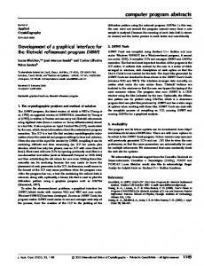
Fig. 1.- Schematic structure of TecD programming. Fig. 1.- Estructura esquemática de la programación de TecD.

al, 2011), and tectonic inferences have to be achieved through tedious counting of samples plotting in different fields and later calculations of success rates in terms of “correctly” classified percentages. Therefore, a suitable computer program could be helpful for an efficient use of such discriminant function based diagrams. We present a new program TecD (Tectonic Discrimination) that enabled us to apply all four sets of five new diagrams for each set (a total of 20 diagrams) to three areas (Faroe Islands in the Atlantic Ocean, Abitibi greenstone belt in Canada, and Mallina basin in Australia). This program will be available to any interested user from request to anyone of the authors ([email protected] or marig@ ier.unam.mx).

169

Verma and Rivera-Gómez / Journal of Iberian Geology 39 (1) 2013: 167-179

2. Computer program TecD was written in VisualBasic (VB.NET). A simplified flow diagram is shown in Figure 1. Basically, a series of options, such as the language, adjusted silica range, and all four sets, or only some sets of diagrams, must first be examined, and a proper selection should be made if the user does not want to process the samples under the default option. The data can be input in an Excel or Statistica file. The program validates the file for possible typographical and other types of errors such as missing variable names or incomplete data. An error-free file is obligatory for using the diagrams, although for a file with incomplete data a suitable selection of diagrams would help. The user can then process the file for different sets of discrimination diagrams (Fig. 1) and save the results as “res” file (all results) or “rep” file (synthesis of results including information on success rates), or both files. The user also has the option to process and save scalable graphics, which can be opened and edited in other conventional software. More details on the functioning and use of TecD in README document (in English as well as Spanish) will be available from the authors. The rocks from four tectonic settings that can be discriminated from these new sets of diagrams are as follows: IAB (island arc basic rocks) numbered as group 1, CRB (continental rift basic rocks) as group 2, OIB (ocean-island basic rocks) as group 3, and MORB (midocean ridge basic rocks) as group 4. A total of 40 equations were programmed in TecD. These are presented according to the papers published in the time sequence from 2004 to 2011 (ADJ in these equations refers to the adjusted data from SINCLAS (Verma et al., 2002) or IgRoCS (Verma and Rivera-Gómez, 2013) computer program; the major oxide symbols refer to oxide concentrations in weight % or % m/m units, e.g., SIO2 stands for SiO2 concentration, i.e., general names, rather than the standardised chemical symbols, were used in these equations; the symbol * is used to show the multiplication operation; function ln stands for natural logarithm; the subscripts m1, m2, t1, and t2 refer, respectively, to the first and second sets of major-element and trace- or immobile element based diagrams). For Agrawal et al. (2004) the equations are as follows. Note these equations use adjusted major-oxide concentrations rather than the crude actually measured values. DF1(IAB-CRB-OIB-MORB)m1 = (0.258*SIO2ADJ) + (2.395*TIO2ADJ) + (0.106*AL2O3ADJ) + (1.019*FE2O3ADJ) - (6.778*MNOADJ) + (0.405*MGOADJ) + (0.119*CAOADJ) + (0.071*NA2OADJ) - (0.198*K2OADJ) + (0.613*P2O5ADJ) - 24.065 (1) DF2(IAB-CRB-OIB-MORB)m1 = (0.730*SIO2ADJ) + (1.119*TIO2ADJ) + (0.156*AL2O3ADJ) + (1.332*FE2O3ADJ) + (4.376*MNOADJ) +

(0.493*MGOADJ) + (0.936*CAOADJ) + (0.882*NA2OADJ) - (0.291*K2OADJ) (1.572*P2O5ADJ) - 59.472 (2) DF1(IAB-CRB-OIB)m1 = (0.251*SIO2ADJ) + (2.034*TIO2ADJ) (0.100*AL2O3ADJ) + (0.573*FE2O3ADJ) + (0.032*FEOADJ) - (2.877*MNOADJ) + (0.260*MGOADJ) + (0.052*CAOADJ) + (0.322*NA2OADJ) (0.229*K2OADJ) - 18.974 (3) DF2(IAB-CRB-OIB)m1 = (2.150*SIO2ADJ) + (2.711*TIO2ADJ) + (1.792*AL2O3ADJ) + (2.295*FE2O3ADJ) + (1.484*FEOADJ) + (8.594*MNOADJ) + (1.896*MGOADJ) + (2.158*CAOADJ) + (1.201*NA2OADJ) + (1.763*K2OADJ) - 200.276 (4) DF1(IAB-CRB-MORB)m1 = (0.435*SIO2ADJ) - (1.392*TIO2ADJ) + (0.183*AL2O3ADJ) + (0.148*FEOADJ) + (7.690*MNOADJ) + (0.021*MGOADJ) + (0.380*CAOADJ) + (0.036*NA2OADJ) + (0.462*K2OADJ) (1.192*P2O5ADJ) - 29.435 (5) DF2(IAB-CRB-MORB)m1 = (0.601*SIO2ADJ) - (0.335*TIO2ADJ) + (1.332*AL2O3ADJ) + (1.449*FEOADJ) + (0.756*MNOADJ) + (0.893*MGOADJ) + (0.448*CAOADJ) + (0.525*NA2OADJ) + (1.734*K2OADJ) + (2.494*P2O5ADJ) - 78.236

(6)

DF1(IAB-OIB-MORB)m1 = (1.232*SIO2ADJ) + (4.166*TIO2ADJ) + (1.085*AL2O3ADJ) + (3.522*FE2O3ADJ) + (0.500*FEOADJ) - (3.930*MNOADJ) + (1.334*MGOADJ) + (1.085*CAOADJ) + (0.416*NA2OADJ) + (0.827*K2OADJ) - 119.050 (7) DF2(IAB-OIB-MORB)m1 = (1.384*SIO2ADJ) + (1.091*TIO2ADJ) + (0.908*AL2O3ADJ) + (2.419*FE2O3ADJ) + (0.886*FEOADJ) + (5.281*MNOADJ) + (1.269*MGOADJ) + (1.790*CAOADJ) + (2.572*NA2OADJ) + (0.138*K2OADJ) - 134.295 (8) DF1(CRB-OIB-MORB)m1 = (0.310*SIO2ADJ) + (1.936*TIO2ADJ) + (0.341*AL2O3ADJ) + (0.760*FE2O3ADJ) + (0.351*FEOADJ) - (11.315*MNOADJ) + (0.526*MGOADJ) + (0.084*CAOADJ) + (0.312*K2OADJ) + (1.892*P2O5ADJ) - 32.909 (9) DF2(CRB-OIB-MORB)m1 = (0.703*SIO2ADJ) + (2.454*TIO2ADJ) + (0.233*AL2O3ADJ) + (1.943*FE2O3ADJ) - (0.182*FEOADJ) - (2.421*MNOADJ) + (0.618*MGOADJ) + (0.712*CAOADJ) - (0.866*K2OADJ) (1.180*P2O5ADJ) - 56.455 (10)

For Verma et al. (2006) the equations are as follows. Note these equations use natural logarithm (ln)-transformed ratios of major oxides using SiO2 as the common denominator for all ratios. Although adjusted data from SINCLAS (Verma et al., 2002) provide essentially the same results, they are certainly useful for ascertaining the basic or ultrabasic nature of magmas before their use in discrimination diagrams. We encourage people to use these (and more recent) diagrams only for such basic and ultrabasic magmas as those inferred from SINCLAS. DF1(IAB-CRB-OIB-MORB)m2 = - 4.6761*ln(TIO2/SIO2) + 2.5330*ln(AL2O3/SIO2) -0.3884*ln(FE2O3/SIO2) + 3.9688*ln(FEO/SIO2) + 0.8980*ln(MNO/SIO2) - 0.5832*ln(MGO/SIO2) 0.2896*ln(CAO/SIO2) - 0.2704*ln(NA2O/SIO2) + 1.0810*ln(K2O/SIO2) + 0.1845*ln(P2O5/SIO2) + 1.5445 (11) DF2(IAB-CRB-OIB-MORB)m2 = 0.6751*ln(TIO2/SIO2) + 4.5895*ln(AL2O3/SIO2) + 2.0897*ln(FE2O3/SIO2) + 0.8514*ln(FEO/SIO2) + -0.4334*ln(MNO/SIO2) + 1.4832*ln(MGO/SIO2) 2.3627*ln(CAO/SIO2) - 1.6558*ln(NA2O/SIO2) + 0.6757*ln(K2O/SIO2) + 0.4130*ln(P2O5/SIO2) +13.1639 (12) DF1(IAB-CRB-OIB)m2 = 3.9998*ln(TIO2/SIO2) - 2.2385*ln(AL2O3/SIO2) + 0.8110*ln(FE2O3/SIO2) - 2.5865*ln(FEO/SIO2) - 1.2433*ln(MNO/SIO2) +

170

Verma and Rivera-Gómez / Journal of Iberian Geology 39 (1) 2013: 167-179

0.4872*ln(MGO/SIO2) - 0.3153*ln(CAO/SIO2) + 0.4325*ln(NA2O/SIO2) 1.0262*ln(K2O/SIO2) + 0.0514*ln(P2O5/SIO2) - 0.5718 (13) DF2(IAB-CRB-OIB)m2 = - 1.3705*ln(TIO2/SIO2) + 3.0104*ln(AL2O3/SIO2)+ 0.3239*ln(FE2O3/SIO2) + 1.8998*ln(FEO/SIO2) - 1.9746*ln(MNO/SIO2) + 1.4411*ln(MGO/SIO2) - 2.2656*ln(CAO/SIO2) + 1.8665*ln(NA2O/SIO2) + 0.2872*ln(K2O/SIO2) + 0.8138*ln(P2O5/SIO2) +1.8202 (14) DF1(IAB-CRB-MORB)m2 = -1.5736*ln(TIO2/SIO2) + 6.1498*ln(AL2O3/SIO2) + 1.5544*ln(FE2O3/SIO2) + 3.4134*ln(FEO/SIO2) - 0.0087*ln(MNO/SIO2) + 1.2480*ln(MGO/SIO2) - 2.1103*ln(CAO/SIO2) - 0.7576*ln(NA2O/SIO2) + 1.1431*ln(K2O/SIO2) + 0.3524*ln(P2O5/SIO2) + 16.8712 (15) DF2(IAB-CRB-MORB)m2 = 3.9844*ln(TIO2/SIO2) + 0.2200*ln(AL2O3/SIO2) + 1.1516*ln(FE2O3/SIO2) - 2.2036*ln(FEO/SIO2) - 1.6228*ln(MNO/SIO2) + 1.4291*ln(MGO/SIO2) - 1.2524*ln(CAO/SIO2) + 0.3581*ln(NA2O/SIO2) 0.6414*ln(K2O/SIO2) + 0.2646*ln(P2O5/SIO2) + 5.0506 (16) DF1(IAB-OIB-MORB)m2 = 5.3396*ln(TIO2/SIO2) - 1.6279*ln(AL2O3/SIO2) + 0.8338*ln(FE2O3/SIO2) - 4.7362*ln(FEO/SIO2) - 0.1254*ln(MNO/SIO2) + 0.6452*ln(MGO/SIO2) + 1.5153*ln(CAO/SIO2) - 0.8154*ln(NA2O/SIO2) 0.8888*ln(K2O/SIO2) - 0.2255*ln(P2O5/SIO2) + 5.7755 (17) DF2(IAB-OIB-MORB)m2 = 1.1799*ln(TIO2/SIO2) + 5.5114*ln(AL2O3/SIO2) + 2.7737*ln(FE2O3/SIO2) - 0.1341*ln(FEO/SIO2) + 0.6672*ln(MNO/SIO2) + 1.1045*ln(MGO/SIO2) - 1.7231*ln(CAO/SIO2) - 3.8948*ln(NA2O/SIO2) + 0.9471*ln(K2O/SIO2) - 0.1082*ln(P2O5/SIO2) + 15.4984 (18) DF1(CRB-OIB-MORB)m2 = - 0.5183*ln(TIO2/SIO2) + 4.9886*ln(AL2O3/SIO2) + 2.2204*ln(FE2O3/SIO2) + 1.1801*ln(FEO/SIO2) - 0.3008*ln(MNO/SIO2) + 1.3297*ln(MGO/SIO2) - 2.1834*ln(CAO/SIO2) - 1.9319*ln(NA2O/SIO2) + 0.6976*ln(K2O/SIO2) + 0.8998*ln(P2O5/SIO2) + 13.2625 (19) DF2(CRB-OIB-MORB)m2 = 5.0509*ln(TIO2/SIO2) - 0.4972*ln(AL2O3/SIO2) + 1.0046*ln(FE2O3/SIO2) - 3.3848*ln(FEO/SIO2) + 0.5528*ln(MNO/SIO2) + 0.2925*ln(MGO/SIO2) + 0.4007*ln(CAO/SIO2) - 2.8637*ln(NA2O/SIO2) 0.2189*ln(K2O/SIO2) - 1.0558*ln(P2O5/SIO2) + 2.8877 (20)

For Agrawal et al. (2008) the equations are as follows. Note these equations use natural logarithm (ln)-transformed ratios of relatively immobile trace elements using Th as the common denominator for all ratios. Also, the first diagram in this set discriminates the combined setting of CRB and OIB from IAB and MORB. Also note that in equations 27 and 28, La/Th ratio is absent because this parameter was not statistically significant for IAB, OIB, and MORB discrimination. SINCLAS computer program (Verma et al., 2002), or still a newer program IgRoCS (Verma and Rivera-Gómez, 2013), must be used to ascertain the basic or ultrabasic nature of magmas before their use in discrimination diagrams. DF1(IAB-CRB+OIB-MORB)t1 = 0.3518*ln(La/Th) + 0.6013*ln(Sm/Th) 1.3450*ln(Yb/Th) + 2.1056*ln(Nb/Th) - 5.4763 (21) DF2(IAB-CRB+OIB-MORB)t1 = - 0.3050*ln(La/Th) - 1.1801*ln(Sm/Th) + 1.6189*ln(Yb/Th) + 1.226*ln(Nb/Th) - 0.9944 (22) DF1(IAB-CRB-OIB)t1 = 0.5533*ln(La/Th) + 0.2173*ln(Sm/Th) 0.0969*ln(Yb/Th) + 2.0454*ln(Nb/Th) - 5.6305 (23) DF2(IAB-CRB-OIB)t1 = - 2.4498*ln(La/Th) + 4.8562*ln(Sm/Th) 2.1240*ln(Yb/Th) - 0.1567*ln(Nb/Th) + 0.94 (24) DF1(IAB-CRB-MORB)t1 = 0.3305*ln(La/Th) + 0.3484*ln(Sm/Th) 0.9562*ln(Yb/Th) + 2.0777*ln(Nb/Th) - 4.5628 (25)

DF2(IAB-CRB-MORB)t1 = - 0.1928*ln(La/Th) - 1.1989*ln(Sm/Th) + 1.7531*ln(Yb/Th) + 0.6607*ln(Nb/Th) - 0.4384 (26) DF1(IAB-OIB-MORB)t1 = 1.7517*ln(Sm/Th) - 1.9508*ln(Yb/Th) + 1.9573*ln(Nb/Th) - 5.0928 (27) DF2(IAB-OIB-MORB)t1 = - 2.2412*ln(Sm/Th) + 2.206*ln(Yb/Th) + 1.2481*ln(Nb/Th) - 0.8243 (28) DF1(CRB-OIB-MORB)t1 = - 0.5558*ln(La/Th) - 1.426*ln(Sm/Th) + 2.2935*ln(Yb/Th) - 0.689*ln(Nb/Th) + 4.1422 (29) DF2(CRB-OIB-MORB)t1 = - 0.9207*ln(La/Th) + 3.652*ln(Sm/Th) 1.9866*ln(Yb/Th) + 1.0574*ln(Nb/Th) - 4.4283 (30)

Finally, for Verma and Agrawal (2011) diagrams, the equations are reported as follows. Note these equations also use natural logarithm (ln)-transformed ratios of relatively immobile major and trace elements using TIO2ADJ (expressed in mg g-1 units rather than wt. % or % m/m, but this change of units is internally executed in TecD) as the common denominator for all ratios. Therefore, in the data file to be processed TiO2 must be input in wt. % as a major element. Also as in Agrawal et al. (2008), the first diagram in this set discriminates the combined setting of CRB and OIB from IAB and MORB. Greater precision is used in these coefficients, because for this set of diagrams the authors have also published probability calculations of individual samples, and the use of higher precision here helps to achieve greater accuracy in these probability estimates. Finally, the prior processing of data in SINCLAS computer program (Verma et al., 2002) is essential for ascertaining the basic or ultrabasic nature of magmas and converting the measured TiO2 into TIO2ADJ. Similarly, the log-transformed ratio variables must also be processed in DODESSYS program (Verma and Díaz-González, 2012; DODESSYS uses the precise and accurate critical values of Verma et al. (2008) for discordancy tests; Barnett and Lewis, 1994) to comply with the basic assumption of normally distributed log-transformed ratios of the samples under study before the use of these newest diagrams. DF1(IAB-CRB+OIB-MORB)t2 = - 0.66107*ln(Nb/TIO2ADJ) + 2.292621*ln(V/TIO2ADJ) +1.677387*ln(Y/TIO2ADJ) + 1.091615*ln(Zr/TIO2ADJ) + 21.36032

(31)

DF2(IAB-CRB+OIB-MORB)t2 = 0.470182*ln(Nb/TIO2ADJ) + 3.764911*ln(V/TIO2ADJ) - 3.91107*ln(Y/TIO2ADJ) + 2.269698*ln(Zr/TIO2ADJ) + 4.848662

(32)

DF1(IAB-CRB-OIB)t2 = - 0.6145999*ln(Nb/TIO2ADJ) + 2.350957*ln(V/TIO2ADJ) +1.682772*ln(Y/TIO2ADJ) + 1.191068*ln(Zr/TIO2ADJ) + 22.72528

(33)

DF2(IAB-CRB-OIB)t2 = 1.37649*ln(Nb/TIO2ADJ) 0.945187*ln(V/TIO2ADJ) + 4.046083*ln(Y/TIO2ADJ) 2.078927*ln(Zr/TIO2ADJ) + 22.24503

(34)

171

Verma and Rivera-Gómez / Journal of Iberian Geology 39 (1) 2013: 167-179

Table 1. Equations of probabilitybased tectonic field boundaries used in the programming of TecD. Tectonic field (boundary type) numbering is as follows: IAB–1; CRB–2; OIB–3; MORB–4; For example, Boundary type 1-2 refers to the probability based boundary that discriminates fields 1 (IAB) and 2 (CRB). Figure numbering (Fig_) refers to these field numbering, and additional information m1, m2, t1, and t2 stands, respectively, for majorelement based first set (Agrawal et al., 2004), major-element based second set (Verma et al., 2006), trace-element based first set (Agrawal et al., 2008), and mainly trace-element based second set (Verma and Agrawal, 2011) of diagrams. For example, Fig_1234m1 means that this is the diagram that discriminates all four tectonic settings of IAB, CRB, OIB, and MORB, and is the first set of major-element based diagram. Further, boundary type also uses a plus (+) sign when the diagram discriminates a combined field of two tectonic settings with the other two fields. For example, the boundary 1-2+3 refers to the boundary of field 1 (IAB) and field 2+3 (CRB and OIB combined field). Tabla 1. Ecuaciones de las fronteras probabilísticas de ambientes tectónicos usadas en la programación de TecD.

Reference / name of diagram set

Agrawal et al. (2004)

Verma et al. (2006)

Agrawal et al. (2008)

Identification of the diagram

Boundary type

Fig_1234m1

1-2 2-3 3-4 1-4 2-4

(–1.03, –8.00) (0.80, 0.32) (0.80, 0.32) (–0.52, –1.03) (–0.52, –1.03)

Fig_123m1

1-2 2-3 1-3

Fig_124m1

Boundary equation Slope (m)

Intercept (b)

(–0.52, –0.99) (8.00, –4.75) (2.67, 8.00) (–8.00, 6.33) (0.80, 0.32)

13.745098 -0.70416667 4.10695187 -0.98395722 1.02272727

6.15745098 0.88333333 -2.9655615 -1.54165775 -0.49818182

(–0.52, 1.34) (–0.52, 1.34) (–0.52, 1.34)

(–2.76, –8.00) (8.00, –5.11) (–1.09, 8.00)

4.16964286 -0.75704225 -11.6842105

3.50821429 0.94633803 -4.73578947

2-4 1-4 1-2

(–0.49, 0.84) (–0.49, 0.84) (–0.49, 0.84)

(–4.97, –8.00) (8.00, –3.04) (–1.93, 8.00)

1.97321429 -0.45700824 -4.97222222

1.806875 0.61606596 -1.59638889

Fig_134m1

1-3 3-4 1-4

(0.50, –2.17) (0.50, –2.17) (0.50, –2.17)

(0.97, –8.00) (4.27, 8.00) (–8.00, 7.10)

-12.4042553 2.69761273 -1.09058824

4.03212766 -3.51880637 -1.62470588

Fig_234m1

2-4 2-3 3-4

(0.50, –2.17) (0.50, –2.17) (0.50, –2.17)

(0.97, –8.00) (4.27, 8.00) (–8.00, 7.10)

2.0175 -0.15836526 -3.23673469

-0.272975 0.09692209 0.6202449

Fig_1234m2

1-2 2-3 3-4 1-4 2-4

(1.160, −0.333) (−0.266, 0.020) (−8.000, −2.490) (1.160, −0.333) (1.160, −0.333)

(5.912, 8.00) (−4.190, 8.00) (−0.266, 0.020) (3.431, -8.00) (−0.266, 0.020)

1.75357744 -2.03363914 0.32454099 -3.37604579 -0.24754558

-2.36714983 -0.52094801 0.1063279 3.58321312 -0.04584712

Fig_123m2

1-2 2-3 1-3

(−0.733, −1.405) (−0.733, −1.405) (−1.343, −8.000)

(−3.788, 8.00) (8.000, 5.428) (−0.733, -1.405)

-3.07855974 0.78243444 10.8114754

-3.66158429 -0.83147555 6.51981148

Fig_124m2

1-2 2-4 1-4

(8.000, −1.332) (−2.673, 8.000) (−6.779,−8.000)

(0.361, −0.619) (0.361, −0.619) (0.361, −0.619)

-0.09333682 -2.84080422 1.0337535

-0.58530541 0.40653032 -0.99218501

Fig_134m2

1-3 3-4 1-4

(−0.830, 1.224) (−0.830, 1.224) (−4.865, −8.000)

(−1.824, 8.000) (8.000, −3.583) (−0.830, 1.224)

-6.81690141 -0.54439411 2.28599752

-4.43402817 0.77215289 3.12137794

Fig_234m2

2-3 3-4 2-4

(0.029, −0.222) (0.029, −0.222) (−0.819, −8.000)

(8.000, 4.322) (−6.177, 8.000) (0.029, −0.222)

0.57006649 -1.32484692 9.17216981

-0.23853193 -0.18357944 -0.48799292

Fig_1234t1

1-2+3 2+3-4 1-4

(-0.12, -8) (8, 7.32) (-8, 5.6)

(-1.03, -0.47) (-1.03, -0.47) (-1.03, -0.47)

-8.27472528 0.86267996 -0.87087518

-8.99296703 0.41856035 -1.36700144

Fig_123t1

1-2 2-3 1-3

(–1.12, 0.71) (–1.12, 0.71) (–1.12, 0.71)

(–2.34, –8.00) (8.00, –2.08) (–1.8, 8.00)

7.13934426 -0.30592105 -10.7205882

8.70606557 0.36736842 -11.2970588

Fig_124t1

1-2 2-4 1-4

(–0.44, –0.39) (–0.44, –0.39) (–0.44, –0.39)

(–1.22, –8.00) (8.00, 3.65) (–7.18, 8.00)

9.75641026 0.47867299 -1.24480712

3.90282051 -0.17938389 -0.93771513

Fig_134t1

1-3 3-4 1-4

(–0.36, –0.78) (–0.36, –0.78) (–0.36, –0.78)

(0.03, –8.00) (8.00, 7.03) (–8.00, 6.06)

-18.5128205 0.93421053 -0.89528796

-7.44461539 -0.44368421 -1.10230367

Fig_234t1

2-3 3-4 2-4 1-2+3 2+3-4 1-4

(0.67, 0.48) (0.67, 0.48) (0.67, 0.48) (0.0282, 8.00) (-3.2318, -8.00) (8.00, -4.5532)

(–8.00, –2.06) (1.58, 8.00) (2.31, –8.00) (0.63849, 0.87812) (0.63849, 0.87812) (0.63849, 0.87812)

0.29296425 8.26373626 -5.17073171 -11.6696652 2.29391596 -0.73779972

0.28371396 -5.0567033 3.94439024 8.32908456 -0.5865224 1.34919774

Fig_123t2

1-2 2-3 3-1

(2.2782, 8.00) (-8.00, 1.6674) (1.876, -8.00)

(0.883172, -0.667465) (0.883172, -0.667465) (0.883172, -0.667465)

6.21311185 -0.26284136 -7.38550383

-6.15471142 -0.43533087 5.85520519

Fig_124t2

1-2 1-4 2-4

(-0.4358, 8.00) (-4.1944, -8.00) (8.00, -5.7992)

(-0.016496, 0.972583) (-0.016496, 0.972583) (-0.016496, 0.972583)

-16.7597185 2.14762785 -0.84473104

0.69611468 1.00801027 0.95864832

Fig_134t2

1-3 1-4 3-4

(-0.8184, 8.00) (8.00, -4.365) (-3.721, -8.00)

(-0.322489, 1.040295) (-0.322489, 1.040295) (-0.322489, 1.040295)

-14.0341815 -0.64948058 2.66007525

-3.48557417 0.83084466 1.89814001

Fig_234t2

2-3 2-4 3-4

(-8.00, 1.485) (3.321, 8.00) (2.43, -8.00)

(1.129586, -0.4194316) (1.129586, -0.4194316) (1.129586, -0.4194316)

-0.2086 3.84200868 -5.82935004

-0.18379997 -4.75931081 6.16532059

Fig_1234t2

Verma and Agrawal (2011)

Boundary coordinates

172

Verma and Rivera-Gómez / Journal of Iberian Geology 39 (1) 2013: 167-179

Area of application

Diagram Reference

Faroe Islands

AGV2004

Faroe Islands

Faroe Islands

Faroe Islands

Abitibi

Abitibi

Abitibi

Mallina

Mallina

Mallina

Mallina

VGA2006

VA2011

VA2011

AGV2008

VA2011

VA2011

AGV2004

VGA2006

AGV2008

VA2011

Number of samples discriminated as CRB+OIB CRB OIB (2+3) (2) (3)

Figure code

Total no. of samples

Fig_1234m1 Fig_123m1 Fig_124m1 Fig_134m1 Fig_234m1

13 13 13 13 13

0 1 0 0

Fig_1234m2 Fig_123m2 Fig_124m2 Fig_134m2 Fig_234m2

13 13 13 13 13

0 0 0 0

Fig_1234t2 Fig_123t2 Fig_124t2 Fig_134t2 Fig_234t2

13 13 13 13 13

Fig_1234t2 Fig_123t2 Fig_124t2 Fig_134t2 Fig_234t2

12 12 12 12 12

Fig_1234t1 Fig_123t1 Fig_124t1 Fig_134t1 Fig_234t1

17 17 17 17 17

Fig_1234t2 Fig_123t2 Fig_124t2 Fig_134t2 Fig_234t2

8 8 8 8 8

Fig_1234t2 Fig_123t2 Fig_124t2 Fig_134t2 Fig_234t2

7 7 7 7 7

Fig_1234m1 Fig_123m1 Fig_124m1 Fig_134m1 Fig_234m1 Fig_1234m2 Fig_123m2 Fig_124m2 Fig_134m2 Fig_234m2 Fig_1234t1 Fig_123t1 Fig_124t1 Fig_134t1 Fig_234t1

11 (6+5) 9 11 (6+5) 11 11 (6+5) 9 11 (6+5) 8 11 (6+5) 11 (6+5) 11 11 (6+5) 11 11 (6+5) 11 11 (6+5) 11 11 (6+5) 11 (6+5) 11 0 11 (6+5) 1 11 (6+5) 11 11 (6+5) 11 11 (6+5) Before and after DODESSYS 11 (6+5) 11 0 11 (6+5) 11 11 (6+5) 11 11 (6+5) 11 11 (6+5)

Fig_1234t2 Fig_123t2 Fig_124t2 Fig_134t2 Fig_234t2

IAB (1)

1 1 9 0 0 0 2 0

Before DODESSYS 12 0 0 0 0

1 12 0

After DODESSYS 12 0 0 0 0

0 12 0

0 0 0 0

0

Before DODESSYS 1 0 3 1 1 After DODESSYS 0 0 2 0 0

1 0 0 5 0

10 11 11 10 12 13 13 13 12 12 12 12 12 12 16 0 0 0 0 0

0

MORB (4) 2 4 2 3

0 0

0 1 0 1 2 0 0 0 9 0 0 0 0 0 0

0 0 0 0 0 0 0 0 0 0 0 0 0 0

Inapplicable

1 11 0 0

Inapplicable

1 1 1 1

Inapplicable

0 1 0 0 17 17 17 17 7 7 7 8 7

5 0

Diagram type

7 7 7

Inapplicable

Inapplicable

Inapplicable

Inapplicable

1 1 3 9 0 0 0 2 0 0 0 11

Inapplicable

Inapplicable

Inapplicable

0 0 0 11

Inapplicable

AGV2004—Agrawal et al. (2004); VGA2006—Verma et al. (2006); AGV2008—Agrawal et al. (2008); VA2011—Verma and Agrawal (2011); Figure code refers to TecD program. The tectonic groups are numbered as follows: IAB─1, CRB─2, OIB─3, MORB─4. For Faroe Islands and Abitibi greenstone belt, one discordant outlier was observed in each case as judged by DODESSYS computer program (Verma and Díaz-González, 2012), also note Verma and Agrawal (2011) diagrams require the log-transformed ratios be normally distributed. For Mallina basin (Australia), both basic and intermediate type of rocks (6 and 5 samples, respectively) provide consistent results and no discordant outliers were detected.

Table 2. Synthesis of inferred tectonic setting results for the three examples presented in this work. Tabla 2. Síntesis de los resultados de los ambientes tectónicos inferidos para los tres ejemplos presentados en este trabajo.

173

Verma and Rivera-Gómez / Journal of Iberian Geology 39 (1) 2013: 167-179

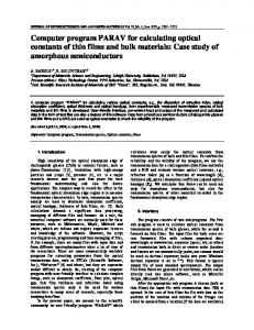
Fig. 2.- The five major-element based diagrams of Agrawal et al. (2004) for the tectonic discrimination of basic and ultrabasic rocks from four tectonic settings (island arc–IAB; continental rift–CRB; ocean island–OIB; and mid-ocean ridge–MORB). The samples plotted are from the Faroe Islands (north Atlantic) and Mallina basin (Australia). DF1 and DF2 are the two discriminant functions obtained from linear discriminant analysis (LDA), and the subscript m1 refers to the first LDA diagram set based on major-element data. Symbols used are shown as an inset in the first diagram. For Mallina, both basic and intermediate rocks were plotted. a) discrimination of all four tectonic settings of IAB, CRB, OIB, and MORB; b) discrimination of three tectonic settings of IAB, CRB, and OIB; c) discrimination of three tectonic settings of IAB, CRB, and MORB; d) discrimination of three tectonic settings of IAB, OIB, and MORB; and e) discrimination of three tectonic settings of CRB, OIB, and MORB. Fig. 2.- Los cinco diagramas de Agrawal et al. (2004) basados en elementos mayores para la discriminación tectónica de rocas básicas y ultrabásicas provenientes de cuatro ambientes tectónicos (arco isla–IAB; rift continental–CRB; isla oceánica–OIB; y dorsal oceánica–MORB). Las muestras graficadas son de las Islas de Faroe (Atlántico norte) y la cuenca de Mallina (Australia). DF1 y DF2 son las dos funciones discriminantes obtenidas del análisis discriminante lineal (LDA), y el subíndice m1 se refiere al primer conjunto de diagramas por LDA, basados en los datos de elementos mayores. Los símbolos usados se muestran en el primer diagrama. Para Mallina ambos tipos de rocas, tanto básicas como intermedias, fueron graficados. a) la discriminación de los cuatro ambientes de IAB, CRB, OIB y MORB; b) la discriminación de tres ambientes de IAB, CRB y OIB; c) la discriminación de tres ambientes de IAB, CRB y MORB; la discriminación de tres ambientes de IAB, OIB y MORB; la discriminación de tres ambientes de CRB, OIB y MORB.

DF1(IAB-CRB-MORB)t2 = - 0.662434*ln(Nb/TIO2ADJ) + 2.449799*ln(V/TIO2ADJ) +1.286697*ln(Y/TIO2ADJ) + 1.091972*ln(Zr/TIO2ADJ) + 18.74662

(35)

DF2(IAB-CRB-MORB)t2 = 0.4937943*ln(Nb/TIO2ADJ) + 3.474124*ln(V/TIO2ADJ) - 3.805286*ln(Y/TIO2ADJ) + 2.006953*ln(Zr/TIO2ADJ) + 3.316333

(36)

DF1(IAB-OIB-MORB)t2 = - 0.2645674*ln(Nb/TIO2ADJ) + 2.049134*ln(V/TIO2ADJ) +3.456482*ln(Y/TIO2ADJ) + 0.8573134*ln(Zr/TIO2ADJ) + 32.94724

(37)

DF2(IAB-OIB-MORB)t2 = 0.01873799*ln(Nb/TIO2ADJ) + 4.093726*ln(V/TIO2ADJ) - 4.854987*ln(Y/TIO2ADJ) + 2.989979*ln(Zr/TIO2ADJ) + 0.1994712

(38)

DF1(CRB-OIB-MORB)t2 = - 0.782930*ln(Nb/TIO2ADJ) + 0.337940*ln(V/TIO2ADJ) +3.323900*ln(Y/TIO2ADJ) - 0.512325*ln(Zr/TIO2ADJ) + 16.094080

(39)

DF2(CRB-OIB-MORB)t2 = 1.7477580*ln(Nb/TIO2ADJ) 0.0421204*ln(V/TIO2ADJ) +3.5300950*ln(Y/TIO2ADJ) 1.4502710*ln(Zr/TIO2ADJ) + 28.3592300

(40)

The coordinates of probability-based boundaries were provided in the original papers (Agrawal et al., 2004, 2008; Verma et al., 2006; Verma and Agrawal, 2011; also see Verma, 2010). To correctly locate the tectonic field in which a given “unknown” sample will plot, it became necessary to accurately calculate each of the boundary equations as done earlier by Verma et al. (2002) for classi-

174

Verma and Rivera-Gómez / Journal of Iberian Geology 39 (1) 2013: 167-179

Fig. 3.- The five major-element based diagrams of Verma et al. (2006) for the tectonic discrimination of basic and ultrabasic rocks from four tectonic settings (island arc–IAB; continental rift–CRB; ocean island–OIB; and mid-ocean ridge–MORB). The samples plotted are from the Faroe Islands (north Atlantic) and Mallina basin (Australia). DF1 and DF2 are the two discriminant functions obtained from linear discriminant analysis (LDA), and the subscript m2 refers to the second LDA diagram set based on major-element data. Symbols used are shown as an inset in the first diagram. For Mallina both basic and intermediate rocks were plotted. a) discrimination of IAB, CRB, OIB, and MORB; b) discrimination of IAB, CRB, and OIB; c) discrimination of IAB, CRB, and MORB; d) discrimination of IAB, OIB, and MORB; and e) discrimination of CRB, OIB, and MORB. Fig. 3.- Los cinco diagramas de Verma et al. (2006) basados en elementos mayores, para la discriminación tectónica de rocas básicas y ultrabásicas provenientes de cuatro ambientes tectónicos (arco isla–IAB; rift continental–CRB; isla oceánica–OIB; y dorsal oceánica–MORB). Las muestras graficadas son de las Islas de Faroe (Atlántico norte) y la cuenca de Mallina (Australia). DF1 y DF2 son las dos funciones discriminantes obtenidas del análisis discriminante lineal (LDA), y el subíndice m2 se refiere al segundo conjunto de diagramas por LDA, basados en los datos de elementos mayores. Los símbolos usados se muestran en el primer diagrama. Para Mallina ambos tipos de rocas, tanto básicas como intermedias, fueron graficados. a) la discriminación de los cuatro ambientes de IAB, CRB, OIB y MORB; b) la discriminación de tres ambientes de IAB, CRB y OIB; c) la discriminación de tres ambientes de IAB, CRB y MORB; la discriminación de tres ambientes de IAB, OIB y MORB; la discriminación de tres ambientes de CRB, OIB y MORB.

fying samples in the TAS diagram. In the DF1-DF2 plots, the equations of the type (DF2=m*DF1+b; where m is the slope, b is the intercept of the corresponding boundary line, and the symbol * stands for multiplication) are summarised in Table 1 for all dividing boundaries. For a given plot, TecD compares the coordinates of an unknown sample with these respective reference boundaries, and decides the exact field in which that sample would plot. Thus, for a given file and a given diagram, all “valid” samples are individually counted and a synthesis is prepared in a report file. TecD thus facilitates an efficient and unequivocal use of all 20 (or less depending on the option used) diagrams for a given geological area. A final report is prepared and provided to the user for help-

ing with the interpretation. 3. Applications Three application examples of TecD are presented for (i) basic rock samples from the Faroe Islands (Atlantic Ocean), (ii) basic and ultrabasic samples from the Abitibi greenstone belt (Canada), and (iii) basic and intermediate rocks from the Mallina basin (Australia). The data are plotted in figures 2-5 and the results from TecD program are summarised in Table 2. We also clarify that although TecD always calculates the success rates in percent (% success rates), we recommend to report only the number of samples plotting in each field when the

Verma and Rivera-Gómez / Journal of Iberian Geology 39 (1) 2013: 167-179

175

Fig. 4.- The five immobile trace-element based diagrams of Agrawal et al. (2008) for the tectonic discrimination of basic and ultrabasic rocks from four tectonic settings (island arc–IAB; continental rift–CRB; ocean island–OIB; and mid-ocean ridge–MORB). The samples plotted are from the Abitibi greenstone belt (Canada) and Mallina basin (Australia). DF1 and DF2 are the two discriminant functions obtained from linear discriminant analysis (LDA), and the subscript t1 refers to the first LDA diagram set based on immobile trace-element data. Symbols used are shown as an inset in the first diagram. For Mallina both basic and intermediate rocks were plotted. a) discrimination of IAB, CRB+OIB, and MORB; b) discrimination of IAB, CRB, and OIB; c) discrimination of IAB, CRB, and MORB; d) discrimination of IAB, OIB, and MORB; and e) discrimination of CRB, OIB, and MORB. Fig. 4.- Los cinco diagramas de Agrawal et al. (2008) basados en elementos mayores, para la discriminación tectónica de rocas básicas y ultrabásicas provenientes de cuatro ambientes tectónicos (arco isla–IAB; rift continental–CRB; isla oceánica–OIB; y dorsal oceánica–MORB). Las muestras graficadas son del cinturón de rocas verdes de Abitibi (Canadá) y la cuenca de Mallina (Australia). DF1 y DF2 son las dos funciones discriminantes obtenidas del análisis discriminante lineal (LDA), y el subíndice t1 se refiere al primer conjunto de diagramas por LDA, basadas en los datos de elementos traza inmóviles. Los símbolos usados se muestran en el primer diagrama. Para Mallina ambos tipos de rocas, tanto básicas como intermedias, fueron graficados. a) la discriminación de los cuatro ambientes de IAB, CRB, OIB y MORB; b) la discriminación de tres ambientes de IAB, CRB y OIB; c) la discriminación de tres ambientes de IAB, CRB y MORB; la discriminación de tres ambientes de IAB, OIB y MORB; la discriminación de tres ambientes de CRB, OIB y MORB.

total number of samples is small, arbitrarily less than 20 (or any other number that the user may decide). 3.1. Paleogene Faroe Islands plateau basalts Søager and Holm (2009) presented new analytical data for 13 high-Ti basalts from the top of the lava pile that was formed presumably by the time of break-up of the North Atlantic about 56–55 Ma ago. These samples were from Faroe Islands located on the eastern continental margin of the Atlantic Ocean. Three of the four sets of tectonic discrimination diagrams (except Agrawal et al. (2008), for which complete data were not available) were applied through TecD for inferring tectonic setting of these lavas.

This application will be described in greater detail than the other two presented in this work. The first diagram (Fig_1234m1 of AGV2004 in Table 2; Fig. 2a) of Agrawal et al. (2004) shows for this area that out of 13 samples of basic and ultrabasic rocks, 10 samples plot in the OIB field, 1 in CRB and 2 in MORB. This diagram, therefore, suggests an OIB setting for the Faroe Islands. The second diagram (Fig_123m1 of AGV2004 in Table 2; Fig. 2b) confirms these results of OIB setting, because 11 out of 13 samples plot in the OIB field. The third diagram (Fig_124m1 of AGV2004 in Table 2; Fig. 2c) is suggested as “Inapplicable” diagram, because the OIB field (field no. 3) is absent from it. The fourth diagram (Fig_134m1 of AGV2004 in Table 2; Fig. 2d) shows once again that

176

Verma and Rivera-Gómez / Journal of Iberian Geology 39 (1) 2013: 167-179

Fig. 5.- The five immobile element based diagrams of Verma and Agrawal (2011) for the tectonic discrimination of basic and ultrabasic rocks from four tectonic settings (island arc–IAB; continental rift–CRB; ocean island–OIB; and mid-ocean ridge–MORB). The samples plotted are from the Faroe Islands (north Atlantic), Abitibi greenstone belt (Canada), and Mallina basin (Australia). DF1 and DF2 are the two discriminant functions obtained from linear discriminant analysis (LDA), and the subscript t2 refers to the second LDA diagram set based on immobile trace-element data. Symbols used are shown as an inset in the first diagram. For Mallina both basic and intermediate rocks were plotted. DiscO stands for discordant outlier detected by the DODESSYS computer program (Verma and Díaz-González, 2012). a) discrimination of IAB, CRB+OIB, and MORB; b) discrimination of IAB, CRB, and OIB; c) discrimination of IAB, CRB, and MORB; d) discrimination of IAB, OIB, and MORB; and e) discrimination of CRB, OIB, and MORB. Fig. 5.- Los cinco diagramas de Verma and Agrawal (2011) basados en elementos inmóviles, para la discriminación tectónica de rocas básicas y ultrabásicas provenientes de cuatro ambientes tectónicos (arco isla–IAB; rift continental–CRB; isla oceánica–OIB; y dorsal oceánica– MORB). Las muestras graficadas son las Islas de Faroe (Atlántico norte), el cinturón de rocas verdes de Abitibi (Canadá) y la cuenca de Mallina (Australia). DF1 y DF2 son las dos funciones discriminantes obtenidas del análisis discriminante lineal (LDA), y el subíndice t1 se refiere al primer conjunto de diagramas por LDA, basados en los datos de elementos traza inmóviles. Los símbolos usados se muestran en el primer diagrama. Para Mallina ambos tipos de rocas, tanto básicas como intermedias, fueron graficados. DiscO significa que los valores en los extremos de arreglo ordenado de datos fueron detectados como discordantes o desviados por el programa de computación DODESSYS (Verma y Díaz-González, 2012). a) la discriminación de los cuatro ambientes de IAB, CRB, OIB y MORB; b) la discriminación de tres ambientes de IAB, CRB y OIB; c) la discriminación de tres ambientes de IAB, CRB y MORB; la discriminación de tres ambientes de IAB, OIB y MORB; la discriminación de tres ambientes de CRB, OIB y MORB.

a large number of samples (11 out of 13) plot in the OIB field. Finally, the fifth diagram (Fig_234m1 of AGV2004 in Table 2; Fig. 2e) also shows 10 out of 13 samples in the OIB field. Thus, all four applicable diagrams (remember one of the five diagrams will generally be inapplicable) show a consistent result, viz., most samples plot in the OIB field. Therefore, we conclude that Agrawal et al. (2004) diagrams suggest an OIB setting for the Faroe Islands. TecD was also used for the application of Verma et al. (2006) major-element based diagrams, which also provided the same results, viz., most samples (12 or 13 out of

13) plot in the OIB field (Table 2 and Fig. 3a-e). The set of diagrams by Agrawal et al. (2008) could not be used for Faroe Islands because of the lack of complete data set (see figure 4a-e, in which samples from Faroe Islands are absent). The application of Verma and Agrawal (2011) diagrams (VA2011 in Table 2; Fig. 5a-e) also gave a consistent result. The first diagram discriminates combined field of CRB and OIB (called “within plate” by many authors; see Verma, 2010), in which an indication of CRB+OIB field was clearly observed. The other three applicable diagrams (Table 2 and Fig. 5b, d, e) also suggest an OIB setting.

Verma and Rivera-Gómez / Journal of Iberian Geology 39 (1) 2013: 167-179

177

The correct use of Verma and Agrawal (2011) diagrams requires that the log-transformed ratios be normally distributed. We achieved this through the use of DODESSYS (Verma and Díaz-González, 2012) by applying all singleoutlier type tests (Barnett and Lewis, 1994; Verma, 1997, 2005; Verma et al., 2009) to log-transformed ratios used in LDA by Verma and Agrawal (2011). We emphasize that discordancy tests should be applied to log-ratios and not to crude compositional data; see Verma (2012) for geochemometric reasons. Only one discordant outlier was obtained, which is plotted by filled diamond symbol in figure 5a-e. This particular sample generally plotted in a field different from the remaining samples, the latter suggested an OIB setting for Faroe Islands. Clearly, an OIB setting is obtained for Faroe Islands. In this case, all four sets of diagrams provided consistent results.

not comment on the probable tectonic setting of these samples, Kerrich et al. (1998) hypothesized an arc setting for the boninite series rocks from this belt of Canada. We also compiled all samples reported by Kerrich et al. (1998). Only 10 out of 18 samples had complete majorelement data set (K2O was missing for the remaining 8 samples). Interestingly, none of these 18 samples proved to be boninite according to the IUGS (International Union of Geological Sciences) scheme of classification (see SINCLAS computer program by Verma et al., 2002). The immobile element based diagrams of Agrawal et al. (2008) also indicated MORB setting for 11 samples of basic and ultrabasic rocks of Kerrich et al. (1998), although the diagrams of Verma and Agrawal (2011) suggested an arc setting (plots not shown) for four basic and ultrabasic rock samples with complete major and trace element data.

3.2. Archaean Abitibi greenstone belt, Canada

3.3. Mallina basin, Australia

Lahaye et al. (1995) presented geochemical data on basic and ultrabasic rocks from the ca. 2700 Ma Abitibi greenstone belt of Ontario, Canada. Major-element data for these samples from Alexo and Texmont areas are incomplete with non-zero Na2O reported for only three (out of 22) samples; besides, for three elements (Na2O, K2O and P2O5) the data seem to be of poor quality. On the other hand, these rocks were probably highly altered as evidenced from their very high water contents as well as from the mineralogical study by Lahaye et al. (1995). Most major-elements for such old rocks might be highly mobile, and therefore the tectonic discrimination will be less reliable. For all these reasons, the major-element based diagrams (Agrawal et al., 2004; Verma et al., 2006) may better be considered as inapplicable. We, therefore, decided to use only immobile element based diagrams (Agrawal et al., 2008; Verma and Agrawal, 2011) whose results are summarised in Table 2. Both sets of diagrams provide consistent results. All samples in figure 4a, c-e plot in the MORB field (Table 2). Note Figure 4b would be the inapplicable diagram because the expected MORB setting is missing from it. Although less number of samples had complete data for figure 5 (Lahaye et al., 1995), most of them plot also in the MORB field (figure 5b is the inapplicable diagram), being consistent with the results of figure 4. Also note that the discordant outlier detected by DODESSYS generally plots in a field different from most of the samples (IAB in Fig. 5a, c, d). Therefore, MORB setting is more likely for the samples from Abitibi greenstone belt of Canada reported by Lahaye et al. (1995). Although Lahaye et al. (1995) did

Smithies (2002) reported the so called boninite-like rocks from the ca. 3010-2935 Ma Mallina basin in the central part of the Pilbara craton (ca. 3120-3115 Ma), northwest Australia. During this long time span (31202935 Ma), both arc and rift settings have been suggested for this area. Smithies (2002) reported major- and traceelement data for 6 boninite-like rocks and 5 melanogabbro rocks. We used TecD to evaluate the tectonic setting of 11 analyses (6 basic and 5 intermediate rock samples, according to the TAS diagram) reported by Smithies (2002). All sets of diagrams (Figs. 2-5) based on major- or trace-elements give consistently an arc setting for these samples (Table 2). With the exception of Agrawal et al. (2004) in which 8-11 samples plot in the IAB field, all sets of diagrams show that all 11 samples (both basic and intermediate types) consistently plot in the IAB setting. No discordant outliers were detected for this dataset. The results remain exactly the same for Verma and Agrawal (2011) diagrams. Therefore, an arc setting can be inferred for the Mallina basin. 4. Final considerations Even though the older binary, ternary and discriminant function based diagrams were not included in TecD because of the deficient statistical handling of compositional data, the newer four sets of five diagrams for each set (a total of 20 diagrams) for basic and ultrabasic magmas (Agrawal et al., 2004, 2008; Verma et al, 2006; Verma and Agrawal, 2011) may be considered too many for ap-

178

Verma and Rivera-Gómez / Journal of Iberian Geology 39 (1) 2013: 167-179

plication to any given area. Nevertheless, when the results of all four sets of diagrams are consistent, there is no problem in the tectonic interpretation based on discrimination diagrams. However, that all four sets provide consistent results might be an exception rather than the rule. We summarise here some guidelines for making decisions in the case of likely inconsistencies (see also Verma et al., 2010). More definitive recommendations for the use of TecD may have to await additional computational work based on Monte Carlo simulations (for more details on Monte Carlo, see Verma, 2012). Sometimes, complete data may not be available for all sets of diagrams to be applied for a given study area. The interpretation in such cases will be limited to the applicable set(s) of diagrams. If one is dealing with relatively old or altered rocks, the two sets of immobile element based diagrams (Agrawal et al., 2008; Verma and Agrawal, 2011) will have to be preferred in comparison to the major-element based diagrams (Agrawal et al., 2004; Verma et al., 2006). On the other hand, for relatively fresh rocks, the diagrams based on major-elements (Agrawal et al., 2004; Verma et al., 2006) will probably be preferable because these elements can generally be determined with less analytical errors than the trace-elements. If the two sets of major-element based diagrams provide inconsistent results, the newer set by Verma et al. (2006) is then preferable, because these diagrams are based on the correct statistical treatment of compositional data. If, on the contrary, the immobile-element based diagrams are mutually inconsistent, there is no simple answer at present, although probably the newer (Verma and Agrawal, 2011) diagrams might be preferable because this set complies additionally with the LDA requirements of normally distributed log-transformed ratio variables used for constructing them. It is also important that this condition be also fulfilled for the application samples, which can be easily achieved from DODESSYS (Verma and DíazGonzález, 2012) or UDASYS software (Verma et al., 2013). Finally, newer diagrams currently under preparation for acid and intermediate magmas should also be applied whenever possible for reaching at the final conclusion from geochemical tectonomagmatic discrimination tools. Acknowledgements The second author (M.A. Rivera-Gómez) is grateful to Conacyt for the fellowship for Master´s studies under the guidance of the first author (S.P. Verma). K. Pandarinath and Sanjeet K. Verma are thanked for using the preliminary versions of TecD and providing suggestions for its improvement. We are also thankful to Alfredo

Quiroz-Ruiz for continuous support and maintenance of our computing facilities essential for the development of our work. We are also much grateful to Prof. Rajesh K. Srivastava and an anonymous reviewer, both of whom greatly appreciated our work and recommended the publication of earlier manuscript in its present form, although we still tried to further improve our presentation through minor corrections of our original manuscript. References Agrawal, S. (1999): Geochemical discrimination diagrams: a simple way of replacing eye-fitted boundaries with probability based classifier surfaces. Journal of the Geological Society of India 54, 335-346. Agrawal, S., Verma, S.P. (2007): Comment on “Tectonic classification of basalts with classification trees” by Pieter Vermeesch (2006). Geochimica et Cosmochimica Acta 71, 3388-3390. doi: 10.1016/j. gca.2007.03.036 Agrawal, S., Guevara, M., Verma, S.P. (2004): Discriminant analysis applied to establish major-element field boundaries for tectonic varieties of basic rocks. International Geology Review 46, 575-594. doi: 10.2747/0020-6814.46.7.575 Agrawal, S., Guevara, M., Verma, S.P. (2008): Tectonic discrimination of basic and ultrabasic rocks through log-transformed ratios of immobile trace elements. International Geology Review 50, 1057-1079. doi: 10.2747/0020-6814.50.12.1057 Aitchison, J. (1986): The statistical analysis of compositional data. Chapman and Hall, London, New York: 416 p. Aitchison, J., Barceló-Vidal, C., Martín-Fernández, J.A., PawlowskyGlahn, V. (2000): Logratio analysis and compositional distance. Mathematical Geology 32, 271-275. doi: 10.1023/A:1007529726302 Armstrong-Altrin, J.S., Verma, S.P. (2005): Critical evaluation of six tectonic setting discrimination diagrams using geochemical data of Neogene sediments from known tectonic settings. Sedimentary Geology 177, 115-129. doi: org/10.1016/j.sedgeo.2005.02.004 Barnett, V., Lewis, T. (1994): Outliers in statistical data. Third edition. John Wiley & Sons, Chichester: 584 p. Cabanis, B., Lecolle, M. (1989): Le diagramme La/10-Y/15-Nb/8: un outil pour la discrimination des séries volcaniques et la mise en évidence des processus de mélange et/ou de contamination crustale. C.R. Acad. Sci. Paris 309, 2023-2029. Kerrich, R., Wyman, D., Fan, J., Bleeker, W. (1998): Boninite series: low Ti-tholeiite associations from the 2.7 Ga Abitibi greenstone belt. Earth and Planetary Science Letters 164, 303-316. doi: 10.1023/A:1007529726302 Lahaye, Y., Arndt, N., Byerly, G., Chauvel, C., Fourcade, S., Gruau, G. (1995): The influence of alteration on the trace-element and Nd isotopic compositions of komatiites. Chemical Geology 126, 43-64. doi: 10.1016/0009-2541(95)00102-1 Pearce, J.A., Cann, J.R. (1971): Ophiolite origin investigated by discriminant analysis using Ti, Zr and Y. Earth and Planetary Science Letters 12, 339-349. doi: 10.1016/0012-821X(71)90220-2 Pearce, J.A., Cann, J.R. (1973): Tectonic setting of basic volcanic rocks determined using trace element analyses. Earth and Planetary Science Letters 19, 290-300. doi: 10.1016/0012-821X(73)90129-5 Pearce, J.A., Harris, N.B.W., Tindle, A.G. (1984): Trace element discrimination diagrams for the tectonic interpretation of granitic rocks. Journal of Petrology 25, 956-983. doi: 10.1093/petrology/25.4.956 Rollinson, H.R. (1993): Using geochemical data: evaluation, presentation, interpretation. Longman Scientific Technical, Essex: 344 p. Shervais, J.W. (1982): Ti-V plots and the petrogenesis of modern and ophiolitic lavas. Earth and Planetary Science Letters 59, 101-118.

Verma and Rivera-Gómez / Journal of Iberian Geology 39 (1) 2013: 167-179 doi: 10.1016/0012-821X(82)90120-0 Sheth, H.C. (2008): Do major oxide tectonic discrimination diagrams work? Evaluating new log-ratio and discriminant-analysis-based diagrams with Indian Ocean mafic volcanics and Asian ophiolites. Terra Nova 20, 229-236. doi: 10.1111/j.1365-3121.2008.00811.x Smithies, R.H. (2002): Archaean boninite-like rocks in an intracratonic setting. Earth and Planetary Science Letters 197, 19-34. doi: 10.1016/S0012-821X(02)00464-8 Søager, N., Holm, P.M. (2009): Extended correlation of the Paleogene Faroe Islands and East Greenland plateau basalts. Lithos, 107: 205215. doi: 10.1016/j.lithos.2008.10.002 Thomas, C.W., Aitchison, J. (2005): Compositional data analysis of geological variability and process: a case study. Mathematical Geology 37, 753-772. doi: 10.1007/s11004-005-7378-4 Vasconcelos-F., M., Verma, S.P., Rodríguez-G., J.F. (1998): Discriminación tectónica: nuevo diagrama Nb-Ba para arcos continentales, arcos insulares, “rifts” e islas oceánicas en rocas máficas. Boletín de la Sociedad Española de Mineralogía 21, 129-146. Vasconcelos-F., M., Verma, S.P., Vargas-B., R.C. (2001): Diagrama TiV: una nueva propuesta de discriminación para magmas básicos en cinco ambientes tectónicos. Revista Mexicana de Ciencias Geológicas 18, 162-174. Verma, S.P. (1997): Sixteen statistical tests for outlier detection and rejection in evaluation of International Geochemical Reference Materials: example of microgabbro PM-S. Geostandards Newsletter. The Journal of Geostandards and Geoanalysis 21, 59-75. doi: 10.1111/j.1751-908X.1997.tb00532.x Verma, S.P. (2005): Estadística básica para el manejo de datos experimentales: aplicación en la Geoquímica (Geoquimiometría). UNAM, México, D.F.: 186 p. Verma, S.P. (2010): Statistical evaluation of bivariate, ternary and discriminant function tectonomagmatic discrimination diagrams. Turkish Journal of Earth Sciences 19, 185-238. doi: 10.3906/yer-0901-6 Verma, S.P. (2012): Geochemometrics. Revista Mexicana de Ciencias Geologícas 29, 276-298. Verma, S.P., Agrawal, S. (2011): New tectonic discrimination diagrams for basic and ultrabasic volcanic rocks through log-transformed ratios of high field strength elements and implications for petrogenetic processes. Revista Mexicana de Ciencias Geológicas 28, 24-44. Verma, S.P., Díaz-González, L. (2012): Application of the discordant out-

179

lier detection and separation system in the geosciences. International Geology Review 54, 593-614. doi: 10.1080/00206814.2011.569402 Verma, S.P., Rivera-Gómez, M.A. (2013): Computer programs for the classification and nomenclature of igneous rocks. Episodes 36, in press. Verma, S.P., Torres-Alvarado, I.S., Sotelo-Rodríguez, Z.T. (2002): SINCLAS: standard igneous norm and volcanic rock classification system. Computers & Geosciences 28, 711-715. doi.org/10.1016/S00983004(01)00087-5 Verma, S.P., Guevara, M., Agrawal, S. (2006): Discriminating four tectonic settings: five new geochemical diagrams for basic and ultrabasic volcanic rocks based on log-ratio transformation of major-element data. Journal of Earth System Science 115, 485-528. doi: 10.1007/ BF02702907 Verma, S.P., Quiroz-Ruiz, A., Díaz-González, L. (2008): Critical values for 33 discordancy test variants for outliers in normal samples up to sizes 1000, and applications in quality control in Earth Sciences. Revista Mexicana de Ciencias Geológicas 25, 82-96. Verma, S.P., Díaz-González, L., González-Ramírez, R. (2009): Relative efficiency of single-outlier discordancy tests for processing geochemical data on reference materials. Geostandards and Geoanalytical Research 33, 29-49. doi: 10.1111/j.1751-908X.2009.00885.x Verma, S.P., Pandarinath, K., Verma, S.K. (2010): Statistically correct methodology for compositional data in new discriminant function tectonomagmatic diagrams and application to ophiolite origin. Advances in Geosciences 27 (Solid Earth Science), 11-22. Verma, S.P., Verma, S.K., Pandarinath, K., Rivera-Gómez, M.A. (2011): Evaluation of recent tectonomagmatic discrimination diagrams and their application to the origin of basic magmas in Southern Mexico and Central America. Pure and Applied Geophysics 168, 1501-1525. doi: 10.1007/s00024-010-0173-2. Verma, S.P., Cruz-Huicochea, R., Díaz-González, L. (2013): Univariate data analysis system: deciphering mean compositions of island and continental arc magmas, and influence of the underlying crust. International Geology Review, in press. doi: 10.1080/00206814.2013.810363. Wood, D.A. (1980): The application of a Th-Hf-Ta diagram to problems of tectonomagmatic classification and to establishing the nature of crustal contamination of basaltic lavas of the British Tertiary volcanic province. Earth and Planetary Science Letters 50, 11-30. doi: 10.1016/0012-821X(80)90116-8