New Design Criteria for Hash Functions and Block Ciphers.

New Design Criteria for Hash Functions and Block Ciphers. by

Prashant Puniya

A dissertation submitted in partial fulfillment of the requirements for the degree of Doctor of Philosophy Department of Computer Science New York University September 2007

Yevgeniy Dodis

c Prashant Puniya

All Rights Reserved, 2007

iv

Abstract Cryptographic primitives, such as hash functions and block ciphers, are integral components in several practical cryptographic schemes. In order to prove security of these schemes, a variety of security assumptions are made on the underlying hash function or block cipher, such as collision-resistance, pseudorandomness etc. In fact, such assumptions are often made without much regard for the actual constructions of these primitives. In this thesis, we address this problem and suggest new, and possibly better, design criteria for hash functions and block ciphers. We start by analyzing the design criteria underlying hash functions. The usual design principle here involves a two-step procedure: First, come up with a heuristically-designed and “hopefully strong” fixed-length input construction (i.e. the compression function), then use a standard domain extension technique, usually the cascade construction (see figure 3.2), to get a construction that works for variable-length inputs. We investigate this design principle from two perspectives: (a) To instantiate the Random Oracle. We suggest modifications to existing constructions that make the resulting construction secure as a random oracle, with appropriate assumptions on the underlying compression function. (b) In general, we look for “black-box” fixes to existing hash functions v

to get secure constructions for each of the common security notions required of hash functions. We also give suggestions for appropriate modes for using existing hash functions along these lines. We next move on to discuss the Feistel network, which is used in the design of several popular block ciphers such as DES, Triple-DES, Blowfish etc. Currently, the celebrated result of Luby-Rackoff [47] (and further extensions) is regarded as the theoretical basis for using this construction in block cipher design, where it was shown that a four-round Feistel network is a (strong) pseudorandom permutation (PRP) if the round functions are independent pseudorandom functions (PRFs). We study the Feistel network from two different perspectives: (a) Is there a weaker security notion for round functions, than pseudorandomness, that suffices to prove security of the Feistel network? (b) Can the Feistel network satisfy a much stronger security notion, i.e. security as an ideal cipher, under appropriate assumptions on the round functions? We give a positive answer to the first question and a partial positive answer to the second question. In the process, we undertake a combinatorial study of the Feistel network, that might be useful in other scenarios as well. We provide several practical applications of our results for the Feistel network.

vi

Contents Dedication . . . . . . . . . . . . . . . . . . . . . . . . . . . . . . . .

iv

Abstract . . . . . . . . . . . . . . . . . . . . . . . . . . . . . . . . .

v

Contents . . . . . . . . . . . . . . . . . . . . . . . . . . . . . . . . .

xi

List of Figures . . . . . . . . . . . . . . . . . . . . . . . . . . . . . . xiii 1 Introduction

1

1.1 Hash Functions . . . . . . . . . . . . . . . . . . . . . . . . . .

2

1.1.1

Hash Functions as Random Oracles . . . . . . . . . . .

3

1.1.2

Getting the Best out of Existing Hash Functions . . . .

9

1.2 Block Ciphers . . . . . . . . . . . . . . . . . . . . . . . . . . . 13 1.2.1

Feistel Networks and Luby-Rackoff’s Result . . . . . . 14

1.2.2

Looking Beyond Pseudorandomness? . . . . . . . . . . 15

1.2.3

An Abstraction for Feistel Networks . . . . . . . . . . . 16

1.2.4

New and Improved Primitives . . . . . . . . . . . . . . 18

1.2.5

The Ideal Cipher Model . . . . . . . . . . . . . . . . . 22

2 Preliminaries

26

vii

2.1 Pseudorandomness and Indistinguishability . . . . . . . . . . . 26 2.2 Ideal Primitives and Indifferentiability . . . . . . . . . . . . . 30 2.3 Other Cryptographic Primitives . . . . . . . . . . . . . . . . . 36

I

2.3.1

Message Authentication Codes . . . . . . . . . . . . . . 36

2.3.2

Collision Resistance . . . . . . . . . . . . . . . . . . . . 37

Hash Functions

39

3 Hash Functions as Random Oracles

40

3.1 Domain Extension for Random Oracles . . . . . . . . . . . . . 48 3.1.1

H(x) = f (h(x)) for Random Oracle f and CollisionResistant One-way Hash-function h . . . . . . . . . . . 48

3.1.2

Plain Merkle-Damg˚ ard Construction . . . . . . . . . . 50

3.1.3

Prefix-free Merkle-Damg˚ ard . . . . . . . . . . . . . . . 51

3.1.4

The Chop Solution . . . . . . . . . . . . . . . . . . . . 53

3.1.5

The NMAC and HMAC constructions

. . . . . . . . . 55

3.2 Constructions using Ideal Cipher . . . . . . . . . . . . . . . . 58 3.2.1

Prefix-free Merkle-Damg˚ ard Construction . . . . . . . . 65

3.2.2

MD-then-Chop Construction . . . . . . . . . . . . . . . 83

3.2.3

NMAC and HMAC Constructions . . . . . . . . . . . . 99

3.2.4

Implications for the RO Domain Extenders . . . . . . . 115

3.3 Other Extensions . . . . . . . . . . . . . . . . . . . . . . . . . 120 4 Getting the Best out of existing Hash Functions viii

123

4.1 Preliminaries . . . . . . . . . . . . . . . . . . . . . . . . . . . 133 4.1.1

Collision Resistance . . . . . . . . . . . . . . . . . . . . 133

4.1.2

Pseudorandomness . . . . . . . . . . . . . . . . . . . . 134

4.1.3

Unpredictability and MACs . . . . . . . . . . . . . . . 134

4.1.4

Target Collision Resistance and One-Wayness . . . . . 135

4.1.5

Randomness Extraction . . . . . . . . . . . . . . . . . 136

4.2 Security of MD modes . . . . . . . . . . . . . . . . . . . . . . 137 4.2.1

Collision Resistance . . . . . . . . . . . . . . . . . . . . 137

4.2.2

Pseudorandomness . . . . . . . . . . . . . . . . . . . . 142

4.2.3

Random Oracle . . . . . . . . . . . . . . . . . . . . . . 148

4.2.4

Message Authentication Code . . . . . . . . . . . . . . 149

4.2.5

Target Collision Resistance . . . . . . . . . . . . . . . . 153

4.2.6

Second Preimage Resistance. . . . . . . . . . . . . . . . 157

4.2.7

Randomness Extraction . . . . . . . . . . . . . . . . . 159

4.2.8

One-Wayness . . . . . . . . . . . . . . . . . . . . . . . 163

4.3 Implications for Actual Hash Functions . . . . . . . . . . . . . 165 4.3.1

Collision Resistance . . . . . . . . . . . . . . . . . . . . 166

4.3.2

Pseudorandomness . . . . . . . . . . . . . . . . . . . . 167

4.3.3

Random Oracle . . . . . . . . . . . . . . . . . . . . . . 167

4.3.4

Message Authentication . . . . . . . . . . . . . . . . . 168

4.3.5

Target Collision Resistance or UOWHFs . . . . . . . . 169

4.3.6

Second Preimage Resistance . . . . . . . . . . . . . . . 169

4.3.7

Randomness Extraction . . . . . . . . . . . . . . . . . 169 ix

4.3.8

II

One-Wayness . . . . . . . . . . . . . . . . . . . . . . . 170

Block Ciphers

171

5 Feistel network made public 5.0.9

172

Luby-Rackoff’s result and Improvements . . . . . . . . 173

5.0.10 The Problem and Our Result . . . . . . . . . . . . . . 175 5.1 Preliminaries . . . . . . . . . . . . . . . . . . . . . . . . . . . 180 5.2 Insecurity of O(log λ)-round Feistel . . . . . . . . . . . . . . . 182 5.3 Combinatorial Analysis of the Feistel Network . . . . . . . . . 184 5.3.1

A “No-Collision” Property of the Feistel Network . . . 185

5.3.2

A Slightly Weaker Result . . . . . . . . . . . . . . . . . 199

5.3.3

Relevance for Feistel Applications . . . . . . . . . . . . 209

6 Implications for Feistel-based Primitives 6.0.4

212

Summary of results . . . . . . . . . . . . . . . . . . . . 213

6.1 Preliminaries . . . . . . . . . . . . . . . . . . . . . . . . . . . 218 6.2 Implications . . . . . . . . . . . . . . . . . . . . . . . . . . . . 223 6.2.1

More Resilient PRPs from PRFs . . . . . . . . . . . . 223

6.2.2

Unpredictable Permutations . . . . . . . . . . . . . . . 230

6.2.3

Verifiable Random Permutations

6.2.4

Verifiable Unpredictable Permutations . . . . . . . . . 239

. . . . . . . . . . . . 237

6.3 Applications . . . . . . . . . . . . . . . . . . . . . . . . . . . . 239 6.3.1

Implications to Domain Extension . . . . . . . . . . . . 240 x

6.3.2

More Resilient Block Ciphers . . . . . . . . . . . . . . 242

6.3.3

Ideal Cipher Model using Semi-Honest Trusted Party . 243

6.3.4

Applications of VRPs/VUPs . . . . . . . . . . . . . . . 245

7 Relation Between the Ideal Cipher and Random Oracle Models

253 7.0.5

Our Plan . . . . . . . . . . . . . . . . . . . . . . . . . 256

7.1 Indifferentiability in the Honest-but-Curious Model . . . . . . 257 7.1.1

Transparent Constructions . . . . . . . . . . . . . . . . 261

7.2 The Construction . . . . . . . . . . . . . . . . . . . . . . . . . 264 7.2.1

Transparency for O(log λ) Rounds . . . . . . . . . . . . 266

7.2.2

HBC Indifferentiability for ω(log λ) rounds . . . . . . . 268

7.2.3

Non-transparency for ω(logλ) rounds . . . . . . . . . . 276

7.2.4

Negative Results for Constant Rounds . . . . . . . . . 277

xi

List of Figures 2.1 The indifferentiability notion: the distinguisher D either interacts with algorithm C and ideal primitive G, or with ideal primitive F and simulator S. Algorithm C has oracle access to G, while simulator S has oracle access to F . . . . . . . . . . 33 2.2 The environment E interacts with cryptosystem P and attacker A. In the G model (left), P has oracle access to C whereas A has oracle access to G. In the F model, both P and A0 have oracle access to F . . . . . . . . . . . . . . . . . . 33 2.3 Construction of attacker A0 from attacker A and simulator S.

35

3.1 The simulator cannot output H(m) since it only receives h(m) and cannot recover m from h(m). . . . . . . . . . . . . . . . . 49 3.2 The plain Merkle-Damg˚ ard Construction . . . . . . . . . . . . 50 3.3 The NMAC and HMAC constructions . . . . . . . . . . . . . . 58 3.4 The Davies-Meyer Compression function . . . . . . . . . . . . 59 4.1 Table for comparing Security Property vs. Mode of operation. 131

xii

5.1 The k-round Feistel Network . . . . . . . . . . . . . . . . . . . 181 5.2 Example of the first three levels of a query tree. All the queries in this example are assumed to be forward queries. . . . . . . 197 7.1 Indifferentiability in honest-but-curious model: The distinguisher D either interacts with CG and gets the transcript TCG ↔F or it interacts with G and gets the simulated transcript TS . . . . . . . . . . . . . . . . . . . . . . . . . . . . . . . . . 259 7.2 An idea of the proof of lemma 24. The conventional honest parties Phon along with the curious ones Pcur can be seen together as a distinguisher D . . . . . . . . . . . . . . . . . . . . 261 7.3 a. Conversion of the simulator S in honest-but-curious model to simulator S 0 in general indifferentiability. b. Conversion of the malicious distinguisher Dmal into an honest-but-curious distinguisher Dcur . . . . . . . . . . . . . . . 264 7.4 Overall Game Structure . . . . . . . . . . . . . . . . . . . . . 276

xiii

Chapter 1 Introduction Cryptographic primitives, such as hash functions and block ciphers, are integral components in the design of practical cryptographic schemes. Often the use of such primitives makes the task of coming up with secure and efficient cryptosystems much easier, as compared to designing such systems from scratch based on complexity-theoretic assumptions. The usual design procedure involves coming up with a proposed construction that uses an abstract function/permutation family. The construction is then proven secure by making an appropriate assumption on the function/permutation family. For instance, assuming the function family to be collision-resistant or assuming the permutations to be pseudorandom permutations. In practice, these functions (resp. permutation) families are instantiated with actual hash functions (resp. block ciphers), in the hope that these constructions will satisfy the required security notion.

1

Hence, depending on the requirements of cryptographic schemes these primitives may need to satisfy a variety of security notions. For this reason, the notion of a “secure” hash function or a “secure” block cipher is a little fuzzy, at best. In this thesis, we attempt to come up with new and possibly better design criteria for these primitives.

1.1

Hash Functions

The most common way of constructing a hash functions consists of two steps. First, one constructs a compression function f : {0, 1}m → {0, 1}n from scratch, or using a block cipher. Then one uses an iterative technique such as the Cascade construction (see figure 3.2) to extend the domain of the function to variable-length inputs. The basic motivation behind using the cascade construction for domain extension was provided by the results of Merkle and Damg˚ ard [22, 54], who showed that the cascade construction applied to a suffix-free encoding1 of the input is collision resistant if the underlying compression function is collision resistant. Thus, the main security notion that has served as a guideline for the design of cryptographic hash functions, such as SHA [32], MD5 [34] etc., has been Collision Resistance. Indeed, these hash functions have been used to instantiate collision resistant functions in a variety of cryptographic schemes. The applications of Collision resistant hash functions (CRHFs) range from 1

In particular, they suggest using the Merkle-Damg˚ ard strengthening, which involves appending the input length to the input

2

signature schemes (the classic “Hash-then-Sign” paradigm), to more recent applications such as those relying on the non-black-box techniques of [2]. However, the problem with using a particular security property as the guideline for hash function design is that now the requirements from hash functions extend to a large number of different security notions. Indeed, hash functions are used as pseudorandom functions, for message authentication, as Universal One-Way Hash Functions (UOWHFs)2 [60], for Key Derivation or even as a Random Oracle [8]. In spite of this large variety of applications, a large fraction of the existing literature related to design and implementation of cryptographic hash functions has concentrated on collision resistance [22, 54, 15]. Apart from this, there have also been results related to pseudorandomness [5], MACs [6, 53], target collision-resistance [11, 70] and key derivation [25].

1.1.1

Hash Functions as Random Oracles

In this thesis, we start by discussing one of the most important applications of hash functions. That is, when hash functions are used to instantiate a random oracle. The random oracle methodology was introduced by Bellare and Rogaway as a “paradigm for designing efficient protocols” [8]. In this paradigm, one designs a cryptographic protocol under the assumption that there exists a ideal random function oracle (RO), which can be accessed by all parties in the protocol (including the adversary). Then one provides a formal 2

also called target collision resistant functions

3

proof of security for the protocol under this assumption. In practice, the random oracle is instantiated using an actual cryptographic hash function, such as one of the hash functions from the SHA family [32]. It is clear that security in the ROM does not guarantee security of the scheme when instantiated with an actual hash functions. Indeed, this was shown in several “separation” results [18, 61, 4, 19, 26] which gave instances of un-instantiable “artificial” cryptographic schemes that are secure in the ROM. However, none of these results gave any attacks on actual schemes that were proven secure in the ROM (such as OAEP [9] or PSS [10]). Thus, the random oracle methodology is still a useful tool for designing efficient cryptographic schemes with “reasonable security guarantee”. In chapter 3, we study the design principles for cryptographic hash functions when used to instantiate the Random Oracle. As we discussed, an actual hash function H : {0, 1}∗ → {0, 1}n is designed to work on variable length inputs. Thus, one would assume that if this hash function H is “random and unstructured” enough, then there should not be any issues with using H for instantiating the random oracle (RO). However, in reality, this thinking is erroneous. As we noted above, practical hash functions are designed by applying a domain extension technique to a fixed-length input compression function f : {0, 1}m → {0, 1}n . While most of the ad-hoc design effort goes into the compression function h, the domain extension technique used in almost all hash functions is the plain Merkle-Damg˚ ard construction (figure 3.2). Thus, 4

it would be unreasonable to expect such a structured construction to behave like a monolithic random oracle. On the other hand, it is a much more difficult task to design a monolithic “unstructured” hash function from scratch. Hence, we approach this problem from a perspective of designing a variable length input random oracle (VIL-RO) from a fixed-length input primitive (for eg., a FIL-RO), so that all the design effort can then be concentrated on coming up with a construction for the fixed-length primitive (in practice, the compression function). We start by noting that none of the previous “domain-extension” results for hash functions (collision-resistance, pseudo-randomness etc.) imply a similar domain extension result for random function oracle. The main reason being that an RO construction must replicate all the properties of the random oracle, such as pseudorandomness, extractability, programmability etc. Since none of the previous definitions guarantee all these properties, it is not even clear how to approach this problem. Indifferentiability We start by discussing what it means to implement an variable-length input random oracle H from a fixed-length building block, such as a FIL-RO f . We show that the notion of indifferentiability introduced by Maurer et al [52] is the right definition in this context. In particular, if we show that the construction H using a fixed-length building block f is indifferentiable from a random oracle under the assumption that f is ideal, then we can use 5

the construction H to instantiate the random oracle in any scheme provably secure in the ROM. And the resulting scheme will be secure in the idealized model corresponding to the primitive f . In order to illustrate this security notion, consider a proposed RO conf struction CH in the f -ideal model. This is an indifferentiable RO construc-

tion if there is a simulator S H that can simulate the role of the fixed-length primitive f in the random oracle model. That is, for any attacker A(·,·) that expects access to two oracles, the following two scenarios are indistinguishable: first, where it has oracle access to the RO H and the simulator S H f and second, where it has oracle access to the RO construction CH and the

fixed-length primitive oracle f . Thus, SH should essentially simulate the role played by the fixed-length primitive f with respect to the RO construction. More details on this definition are given in chapter 2, section 2.2. Domain Extension for Random Oracle Equipped with a suitable definition, we attempt to find an indifferentiable construction of a variable-length random oracle H from a fixed-length random function oracle f 3 . We start by discussing some existing, and seemingly secure domain extension techniques under this definition. In particular, we show that the popular hash-then-sign paradigm is not secure in this context. Moreover, even the plain Merkle-Damg˚ ard construction, used in almost all existing hash functions, is not an indifferentiable 3

This is a fixed-length random function that is accessible to all the parties in the protocol.

6

construction of a VIL-RO (even with Merkle-Damg˚ ard strengthening). Thus, the existing design principle behind hash functions such as SHA-1 or MD5 is not secure for our goal. Therefore, instead of giving new and practically unmotivated constructions, we come up with minimal changes to the plain Merkle-Damg˚ ard construction that are easily implementable in practice, and satisfy our security definition. In particular, we propose the following modifications to the plain MD construction: 1. Prefix-free encoding: we show that if the inputs to the plain MD construction are guaranteed to be prefix-free, then the resulting construction is secure. 2. Dropping some output bits: we show that by dropping a non-trivial number of output bits from the output of the plain MD construction, we get an indifferentiable construction of a VIL-RO. 3. The NMAC construction (see figure 3.3a): we show that by applying an independent hash function g to the output of the plain MD construction using f (as in the NMAC construction [5]), then we get an indifferentiable VIL-RO construction in the random oracle model for f and g. 4. The HMAC construction (see figure 3.3b): we show a slight variant of the NMAC construction allows us to build the second function g from f itself (as in [5], in going from NMAC to HMAC)! In this latter 7

variant, one implements a secure hash function H by making two blackbox calls to the plain MD construction (with the same IV and a given compression function f ). Ideal Cipher to Random Oracle In practice, most hash functions are block-cipher based, either explicitly as in [15] or implicitly as in SHA-1. Therefore, we consider the question of constructing a VIL-RO H from an ideal block cipher E : {0, 1}κ × {0, 1}n → {0, 1}n . An ideal block cipher is an ideal primitive that takes a κ-bit key, and defines an independent random permutation for each key. We concentrate on using the Merkle-Damg˚ ard construction with the DaviesMeyer compression function f (x, y) = Ey (x) ⊕ x, since this is the most practically relevant construction. One could hope to first show that the DaviesMeyer compression function is an indifferentiable construction of a FIL-RO in the ideal cipher model for E and then use one of the secure constructions of a VIL-RO from a FIL-RO. However, as we show, this first attempt fails and the Davies-Meyer construction fails to give a FIL-RO from an ideal cipher. Fortunately, we show, via direct proofs, that all four fixes proposed for FIL-RO to VIL-RO construction also work when used with the Davies-Meyer compression function in the ideal cipher model.

8

1.1.2

Getting the Best out of Existing Hash Functions

Having discussed the use of hash functions for instantiating the random oracle, we then analyze security of hash functions in a more general perspective. As we mentioned above, hash functions are required to satisfy a variety of different security requirements in cryptographic schemes. In fact, in the past, hash functions were viewed by practitioners as black-boxes with magic properties. However, this perception has changed since the recent attacks on existing hash functions, including the SHA-1 and MD5. Most notable of these were the new and improved collision-finding attacks proposed by Wang et al [72, 73]. Along with other results demonstrating weaknesses of existing hash function constructions, such as [43, 45], these attacks showed that the collision-resistance of these hash functions is much worse than what was anticipated earlier. Moreover, these results have also cast a doubt on the security of these hash functions with respect to other notions. These results have prompted NIST into organizing a series of workshops [62] for coming up with constructions for the “next generation” hash functions, and rightly so. However, this new standard is not expected to be decided any time soon. Meanwhile, practitioners are stuck with either using existing, known to be “insecure”, hash functions or using an ad-hoc implementation that has not undergone the thorough analysis that standardized hash functions go through. In either case, the resulting application will be prone to possible weaknesses that are avoidable. 9

In chapter 4, we address this problem by looking for fixes that would allow practitioners to use standardized hash functions while side-stepping several of the weaknesses of existing constructions. As we have discussed, almost all existing hash functions are based on the plain MD construction (with Merkle-Damg˚ ard strengthening). Thus, we look for black-box fixes that can be implemented on top of the plain MD construction for several of the applications that hash functions are often used for. Efficient Black-Box Fixes to Existing Hash Functions Most of the prior work for hash functions has been aimed at finding iterative techniques (usually, some variants of the plain MD construction) for extending the domain of fixed length primitive to get an arbitrary length primitive satisfying the same security property, which are also often called property-preserving transforms. For instance, the results from chapter 3 for constructing a VIL-RO from a FIL-RO fall under this category. However, we note that it is not always the case that these variants of the plain MD construction can be implemented on top of a plain MD based hash function. An example in this context is the PRF domain extension technique in [5]. In fact, most often the reason for such “non-black-box variants” of the plain MD construction is that no black-box variants are known that preserve the required security property. In chapter 4, our focus will be slightly different in the sense that we will emphasize this alternative goal for domain extension techniques more than 10

property preservation. In particular, we are willing to make slightly stronger assumptions on the fixed-length primitive in order to get a variable-length primitive with a desired security property. We will look for efficient variants of the plain MD construction that satisfy the following axioms: 1. It should consist of one or two “black-box” calls to plain MD construction. 2. The construction must support variable-length inputs. 3. Compared to a single evaluation of the plain MD construction, its evaluation should make at most a fixed (small constant) number of extra calls to the underlying compression function. Such a variant of the plain MD construction will allow a practitioner, who understands the security property he/she needs from the hash functions, to use an existing standardized implementation without having to tinker with the, often rather involved, internals of the implementation. We also refer to such a variant of the plain MD construction as an efficient black-box hash function mode of operation. Security Properties vs. Modes of Operation The axioms that we require our hash function modes of operation to satisfy leave very little choice for the domain extension techniques that one can use. We discuss most of the popular hash function modes of operation that satisfy our axioms: 11

1. Plain MD Construction: This captures the notion that the application uses the hash function as it is. 2. Encode-then-MD Construction: In this case, the user encodes the hash function input before applying the plain MD construction. Examples of popular encoding schemes used are suffix-free encoding and prefix-free encoding. 3. MD-then-Chop Construction: Here the user applies the plain MD mode and only uses part of the output while discarding the remaining bits. In particular, existing hash functions SHA-224 and SHA-384 are obtained this way from SHA-256 and SHA-512, respectively. 4. NMAC/HMAC Construction: The version of the NMAC construction that we consider simply composes two applications of the plain MD mode with possibly different initialization vectors IV1 and IV2 . While not obeying the first axiom, the NMAC construction serves as a nice abstraction for the HMAC construction which does satisfy all our axioms (but is slightly harder to formally analyze in some cases). Essentially, the HMAC construction simulates the two black-box calls of the NMAC construction with different IV s, by adding prefixes to the input in each call. We analyze each of these hash function modes of operation for most of the security properties that are usually desired of hash functions. The hash function properties that we analyze include: (1) Collision-resistance, (2) Pseu12

dorandomness, (3) Message Authentication, (4) Random Oracle, (5) Target Collision Resistance (UOWHFs), (6) Second Preimage Resistance, (7) Randomness Extraction, and (8) One-Wayness. In each case, we find the minimal assumptions that one needs to make on the compression function in order to achieve the required security property from the resulting hash function mode of operation. In many cases, it turns out that we need to make stronger assumptions on the compression function than the desired security property. Some of these results follow directly from previous work, while for other results we provide separate proofs in chapter 4. We provide a detailed “security property vs. hash function mode of operation guide” that gives the minimal assumptions one needs to make on the compression function for each of an efficient black-box mode of operation to satisfy each of the security property (see figure 4.1). This will serve as a useful guide for practitioners on how to use existing hash functions when they desire a certain security property from them.

1.2

Block Ciphers

In the second part of this thesis, we discuss another important cryptographic primitive, a block cipher. A block cipher E : {0, 1}κ ×{0, 1}n → {0, 1}n takes a κ-bit key, and gives a permutation on n-bit strings for each key. Examples of actual block ciphers include Data Encryption Standard (DES), Advanced

13

Encryption Standard (AES) etc. The initial use of block ciphers was for symmetric key encryption. Though the uses for block ciphers are not as wide-ranging as in the case of hash functions, these primitives are also used in several scenarios other than for privacy. For instance, these are used in the popular message authentication mode, CBC-MAC, or in instantiating schemes in the ideal cipher model [15, 23, 30, 42, 46].

1.2.1

Feistel Networks and Luby-Rackoff ’s Result

Feistel networks form the basis of several block cipher constructions, such as DES, Triple DES, Blowfish etc. A Feistel network consists of multiple iterative applications of the Feistel transform. The Feistel transform provides a construction of a permutation on 2n-bit strings using a length-preserving def

function f : {0, 1}n → {0, 1}n . It is defined as follows: Ψf (x) = xR k (xL ⊕ f (xR )). The different iterative applications of the Feistel transform are known as the rounds of the Feistel network, and the corresponding functions are called round functions. Initially, there was no theoretical justification for the usage of the Feistel networks in the design of block ciphers. This theoretical justification was provided by the result of Luby and Rackoff [47], who showed that 4 rounds of the Feistel network with independent pseudorandom functions in each round gives a (strong) pseudorandom permutation 4 . Since the paper of Luby4

A strong pseudorandom permutation is indistinguishable from a truly random permu-

14

Rackoff, several improvements were made to their result (see [58, 51, 69, 64]). All these results showed essentially argued the pseudorandomness of a multiple round Feistel network with pseudorandom round functions (with improving exact security of the reductions or under slightly different attack scenarios). These results provided enough justification for the use of the Feistel network based block ciphers for symmetric key encryption. Indeed, pseudorandomness of ciphertexts is the security property that one desires from a symmetric key encryption scheme.

1.2.2

Looking Beyond Pseudorandomness?

However, there are several reasons to look for other security properties from block ciphers. (a) As we mentioned above, block ciphers are utilized for a much wider range of applications than for symmetric key encryption alone. These applications often require security properties that may be different from pseudorandomness. (b) The round functions (or S-Boxes in actual constructions) in Feistel network based block ciphers are designed based on heuristics, and may not be (possibly even close to) pseudorandom functions. In this case, all of the previous results for the Feistel network become inapplicable. (c) Moreover, the round functions in actual constructions may leak a lot of tation for any attacker that can make both forward or inverse permutation queries

15

information about the intermediate round values of the Feistel network. Again, all of the prior results for Feistel networks assume the secrecy of all (or at least some) of the round values. In part II of this thesis, we analyze the Feistel networks from this perspective. In particular, we analyze the Feistel network under both weaker as well as stronger security notions than pseudorandomness. Firstly, we analyze the situation when the round functions of a Feistel network are not pseudorandom functions. In particular, we analyze the situation when the round functions satisfy some weaker security property than pseudorandomness, or if the intermediate round values of the Feistel network are somehow (possibly thorough weakness of round functions) leaked to the attacker. We give positive results in such a situation in chapter 6. Secondly, we ask if the Feistel network could be used to design a much stronger primitive than a pseudorandom permutation. That is, we analyze if, under some (ideal) security assumption on the round functions, the Feistel network is an indifferentiable construction of an ideal block cipher. Note that this is also the other direction of one of the questions addressed in chapter 3. We give a partial positive answer to this question in chapter 7.

1.2.3

An Abstraction for Feistel Networks

As we discussed, most of the previous results become inapplicable if either the round functions are not pseudorandom, or (at least some of) the round

16

values are not hidden from the attacker. In order to handle this problem, we start out by discussing a combinatorial abstraction for the multiple round Feistel network that is applicable to scenarios where one or both of these assumptions do not hold. In particular, we do not make any assumptions on the round functions when stating this result. Consider a k-round Feistel network that defines a permutation on 2n bits based on k length-preserving functions on n-bits. We will refer to the inputs to each of these round functions as the round values of the Feistel network. We study a game between this k-round Feistel network and an attacker that makes 2n-bit forward/inverse permutation queries to this Feistel network and gets the result as well as all the intermediate round values. The attacker wins the game if it makes two queries such that the middle ((k/2)th ) round values in these queries collide. We show that if the attacker wins after making q queries to the k-round Feistel network in this game, then: (a) Either the number of queries, q, made by it is exponential in k. (b) Or a new round function output can be represented as an XOR of upto 5 other round values that already existed before this round function output. We refer to this as the 5-XOR condition (see section 5.1). The second condition essentially implies that for some query made by the attacker, a round function, say fi (Ri ), where output can be represented as an XOR of upto 5 round values that were defined before this round function 17

output. This includes round values from earlier queries, or round values from this query that were defined before this round function output. This property essentially proves a property of an interaction between an attacker and the Feistel network that does not depend on the round functions used in the construction. We use this property for our problem by showing that if the round functions of the Feistel network are chosen such that the 5-XOR condition is not satisfied for any efficient attacker, then the number of queries made by a “winning” attacker must be exponential in the number of rounds k (which is super-polynomial in the security parameter λ for k = ω(log λ). Moreover, we show that this result is tight in the sense that for a Feistel network with upto logarithmic number of rounds k = O(log λ), there is an attacker that can find the input corresponding to any permutation output by making only forward queries. This is sufficient to see that the combinatorial property above does not hold for such a Feistel network. In fact, as we show in chapter 6, this implies that such a Feistel network is not useful for most applications where the round values are revealed to the attacker.

1.2.4

New and Improved Primitives

In chapter 6, we show new (or improved) constructions of some cryptographic primitives using the combinatorial property above. First, prove a stronger result than Luby-Rackoff (and subsequent results) for PRPs, that with a super-logarithmic number of rounds, the Feistel network, with independent 18

PRFs as round functions, is a (strong) pseudorandom permutation even if the PRP attacker can observe the intermediate computations of the Feistel network. This gives a more resilient PRP construction. Coming back to our first question, we ask if there is a weaker property of the round functions than pseudorandomness, that guarantees some security property for the Feistel network. We show that even if the round functions of a super-logarithmic round Feistel network are only unpredictable functions (UFs) then it is an unpredictable permutation (UP) 5 . In fact, we show that this result is tight, in the sense that for upto a logarithmic number of rounds, there is a set of UFs that do not give a UP via the Feistel network (see lemma 23). Next, we show that our result is also useful in a scenario where the application may need to explicitly reveal all the intermediate round values to an attacker. For instance, this comes up when one tries to add verifiability to the PRP or UP constructions above. The notion of verifiable (pseudo)random functions (VRFs) was introduced by Micali et al. [55]. These are essentially verifiable analogs of PRFs, with a public key P K and secret key SK. Given both the public and secret keys, one can compute the output y of the VRF on an input x, as well as construct a short proof that y is indeed the output of the VRF on input x and not some “garbage value” (which could easily be done for a normal PRF). On the other hand, given only the public key P K, 5 Roughly speaking, an unpredictable function guarantees that no attacker can predict the output of the function on an unqueried input (similarly for unpredictable permutations with both forward/inverse queries).

19

one can verify this proof to learn whether y is indeed the correctly computed output (see formal defns. in section 6.1). We introduce the notion of verifiable (pseudo)random permutations (VRPs) that are similar verifiable analogues of PRPs (or permutation analogues of VRFs). For VRPs, one can compute (and provide proofs for) both the forward and inverse permutation given the public and secret keys. We show that a super-logarithmic round Feistel network with independent VRFs as round functions, is a secure VRP. Note that in this case, the VRP proof will simply consist of intermediate round function input/output pairs along with the corresponding VRF proofs. Thus the round values need to be revealed to the attacker, which makes all of the previous techniques for the Feistel network inapplicable. Moreover, this also implies that super-logarithmic number of rounds are both necessary and sufficient. Finally, we consider the case of verifiable unpredictable permutations (VUPs). These are verifiable analogs of unpredictable permutations. The corresponding notion of verifiable unpredictable functions (VUFs) was also introduced by Micali et al. [55]. These are also known as unique signatures (see [38, 49]). Micali et al. used VUFs as an intermediate step for constructing VRPs. Note that in this case, if one uses the Feistel network with VUFs as round functions to construct VUPs, then neither are the round functions pseudorandom, nor are the round values hidden from the attacker (and are revealed as part of the VUP proof). However, we show that even in this case, a super-logarithmic round Feistel network is both necessary and sufficient to 20

construct VUPs from VUFs. Applications We then provide various examples of natural scenarios where our technique (and the constructions we derive from it) are useful. These applications are described in section 6.3 (chapter 6). • We show how our results provide a “closer-to-reality” justification for the number of Feistel rounds heuristically used in practical block cipher constructions. • Using our results, we provide the most efficient domain extension technique for length-preserving MACs without introducing any new assumptions. • We show that VRPs immediately yield non-interactive, setup-free, perfectlybinding commitment schemes. • VRPs can be used to fix a subtle security flaw in the non-interactive lottery system of Micali-Rivest [56]. • We show that these primitives can also be used to implement so called “invariant signatures” needed by Goldwasser and Ostrovsky [38]. • Other applications of VRPs, such as verifiable CBC encryption/decryption, verifiable huge (pseudo)random objects [36] or a “proof-transferable”

21

implementation of the Ideal Cipher Model using a semi-trusted third party.

1.2.5

The Ideal Cipher Model

In chapter 7, we analyze if the Feistel network can be used to achieve a stronger security notion than pseudorandomness. That is, we analyze if the Feistel network can be used to get an indifferentiable construction of the ideal cipher (IC) from a random oracle (RO). This is essentially the converse of a question we studied in chapter 3. There we gave indifferentiable constructions of the random oracle from the ideal cipher oracle. If the converse result also holds, then it will also imply that the ideal cipher model (ICM) is equivalent to the random oracle model (ROM). Although, the ideal cipher model has not been as widely applicable as the random oracle model, there have been some results that utilize this model (see [15, 23, 30, 42, 46]). We give a “partial positive” answer to this question, by showing that with sufficient number of rounds a Feistel network based construction using RO is indifferentiable from the ideal cipher in the “honest-but-curious” model. This is a weaker security notion than general indifferentiability, that is still stronger than classical indistinguishability (that is used in the case of PRPs). Indifferentiability in the Honest-but-Curious Model We start out by introducing the notion of indifferentiability in the honestbut-curious model in section 7.1. In order to illustrate this security notion, 22

consider a construction CEH of the IC E using the RO H. Under the general notion of indifferentiability this construction is a secure ideal cipher construction, if there is an efficient simulator that can simulate the role of the RO H in the ideal cipher model. In this weaker notion, the task of the simulator is simply to simulate the interaction between the RO H and the construction CEH in the ideal cipher model. That is, for any attacker A that has expects access to the ideal cipher construction oracle CEH and can make queries to this construction where it observes the queries that CEH , in turn, makes to the random oracle H, the following two scenarios are indistinguishable: first, where it has oracle access to CEH and can observe the actual interaction between CE and H or second, where it has oracle access to the ideal cipher E and the simulator S generates a fake interaction for the attacker. We show that if an ideal cipher construction is indifferentiable in the honest-but-curious model, then any cryptographic protocol that is secure against honest-but-curious attackers in the ideal cipher model can also be instantiated in the random oracle model using this construction. Next, we define the notion of a transparent construction, which are constructions for which general indifferentiability is equivalent to indifferentiability in the honest-but-curious model. Roughly speaking, for a transparent ideal cipher construction using RO, an attacker can query the RO indirectly by making queries to the construction and observing its interaction with the RO.

23

An HBC Indifferentiable construction and going beyond. . . Next, we analyze the Feistel network to find out if it can give us an indifferentiable IC construction using RO. We first show that for upto a logarithmic number of rounds k = O(log λ), the k-round Feistel network is a transparent construction. That is, if one can prove the honest-but-curious indifferentiability of this construction, then it will also imply general indifferentiability. This implies that if such a k-round Feistel network is an HBC indifferentiable ideal cipher construction, then the random oracle model and the ideal cipher model are equivalent! We conjecture that this is the case and that in fact, even a 6-round Feistel network might be an indifferentiable ideal cipher construction. However, we have not been able to come up with a formal proof of this conjecture. However, we show that with super-logarithmic number of rounds k = ω(log λ), the k-round Feistel network is HBC indifferentiable from the ideal cipher. This result uses the combinatorial property that we prove in chapter 5. This would indicate that one might be able to show that such a construction is indifferentiable from the ideal cipher in general, by showing that this is a transparent construction. Unfortunately, we prove that this cannot be the case by showing that for super-logarithmic number of rounds, the Feistel network cannot be a transparent construction. Thus, in this case, honest-but-curious indifferentiability is a strictly weaker notion than general indifferentiability. Finally, we state a result of Coron [20] who shows that for upto 5 rounds, 24

the Feistel network does not even give an HBC indifferentiable ideal cipher construction. We give a proof of this fact for a 4-round Feistel network in section 7.2.4. This result also implies that the notion of indifferentiability in the honest-but-curious model is strictly stronger than classical indistinguishability, since 4 rounds are sufficient in the latter case [47].

25

Chapter 2 Preliminaries 2.1

Pseudorandomness and Indistinguishability

Let λ ∈ N denote the security parameter. Let {Aλ , Bλ }λ∈N be a sequence of pairs of sets. For the purposes of this thesis, Aλ and Bλ will be of the form {0, 1}n(λ) and {0, 1}m(λ) , respectively. Here n(·) and m(·) are polynomial functions N 7→ N. When no ambiguity can arise, we will simply represent these sets as {0, 1}n and {0, 1}m . Let Fλ be the set of all functions Aλ 7→ Bλ , and let Pλ be the set of all permutations on Aλ . A function ensemble H = {Hλ }λ∈N is a sequence such that each Hλ is distributed on Fλ . Here H is the uniform function ensemble if Hλ is uniformly distributed on Fλ . A permutation ensemble H = {Hλ }λ∈N is a sequence such that each Hλ is distributed on Pλ , and H is the uniform 26

permutation ensemble is Hλ is uniformly distributed on Pλ . A function ensemble is efficiently computable if the distribution Hλ is efficiently samplable and the functions in Hλ can be computed efficiently. That is, there exist probabilistic polynomial time Turing machines, I and V , and a mapping from strings to functions, φ, such that (1) φ(I(1λ )) and Hλ are identically distributed and (2) V (i, x) = (φ(i))(x) so that V (I(1n ), ·) is def

essentially Hλ (·). We denote by fi the function assigned to i (i.e. fi = φ(i)). We refer to i as the key of fi and to I as the key generating function of F . Throughout this thesis, when we consider function (or permutation en sembles), the sequence of sets {Aλ , Bλ }λ∈N will be of the form {0, 1}n(λ) , {0, 1}m(λ) , where n, m are functions on N 7→ N. The usual key generation

function I will simply output a uniformly sampled random bit string from a set {0, 1}k(λ) , i.e. I(1λ ) is uniformly distributed over {0, 1}k(λ) . We start by describing the notion of indistinguishability of two function (or permutation) ensembles. In this notion, the distinguisher is an oracle

machine that is given oracle access to a function in Fλ or a permutation in Pλ . On input 1λ , the distinguisher makes queries to the function or permutation that it has oracle access to, and outputs a single bit. We assume that on input 1λ , the distinguisher only makes queries in Aλ . For the purpose of this thesis, the oracle machine can be thought to be an oracle Turing machine. Let D be an oracle machine, let f be a function in Fλ and let Hλ be distributed over Fλ . We denote by D f (1λ ), the output distribution of D when its oracle queries are answered by f , and denote by D Hλ (1λ ), the output dis27

tribution of D when its oracle queries are answered by a function distributed according to Hλ . We will also consider oracle machines that take oracle access to a permutation in Pλ and its inverse. Let π be a permutation in Pλ −1

and let Hλ be a distribution over Pλ . We denote by D π,π (1λ ), the output distribution of D when it is given oracle access to the permutation π, and −1

denote by D Hλ ,Hλ (1λ ), the output distribution of D when it is given oracle access to a permutation distributed according to Hλ . ˜ = Definition 1 ((t, q, )-indistinguishability). Let H = {Hλ }λ∈N and H ˜ λ }λ∈N be two function ensembles. We say that H and H ˜ are (t, q, ){H indistinguishable function ensembles if for any probabilistic oracle machine D running in time t and making at most q oracle queries,  i h  ˜λ λ H Hλ λ Pr D (1 ) = 1 − Pr D (1 ) = 1 ≤  Here t, q and  are all functions of the security parameter λ. The same definition can also be used for (t, q, )-indistinguishability of two permutation ˜ H ˜ −1 i. ensembles hH, H −1 i and hH, Definition 2 (negligible function). A function h : N → N is negligible if for every constant c > 0 and all sufficiently large n,

h(n)
n), getting the final output. Note that we could also define the HMAC construction by using a different initialization vector in each part of the construction, instead of using the same IV but prepending 0κ to the input. However, our purpose here is to present these constructions as black-box extensions of existing hash functions such as SHA-1 which have only one fixed IV , in which case our proposed construction can be viewed as making two black-box calls to SHA-1 to get SHA − 1(SHA − 1(0κ k m1 . . . m` ). However, in practice most hash-function constructions are block-cipher based, either explicitly as in [68] or implicitly as for SHA-1. Therefore, we consider the question of designing an arbitrary-length random oracle H

47

from an ideal block cipher E, specifically concentrating on using the MerkleDamg˚ ard construction with the Davies-Meyer compression function f (x, y) = Ey (x) ⊕ x, since this is the most practically relevant construction. We show that all of the four fixes to the plain MD chaining which worked when f was a fixed-length random oracle, are still secure (in the ideal cipher model) when we plug in f (x, y) = Ey (x) ⊕ x instead. Specifically, we can either use a prefix-free encoding, or drop a non-trivial number of output bits (when possible), or apply an independent random oracle g to the output of plain MD chaining, or use the optimized HMAC construction which allows us to build this function g from the ideal cipher itself.

3.1

Domain Extension for Random Oracles

In this section, we show how to construct an iterative hash-function indifferentiable from a random oracle, from a compression function viewed as a random oracle. We start with two simple and intuitive constructions that do not work.

3.1.1

H(x) = f (h(x)) for Random Oracle f and CollisionResistant One-way Hash-function h

One could hope to emulate a random oracle (with arbitrary-length input) by taking : C f (x) = f (h(x)) 48

f C h C(m)

f =

f(h(m))

H

S

H(m)

= S(h(m))

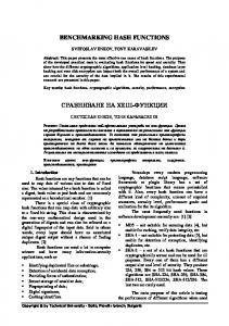
Figure 3.1: The simulator cannot output H(m) since it only receives h(m) and cannot recover m from h(m). where f : {0, 1}n → {0, 1}n is modelled as a random oracle and h : {0, 1}∗ → {0, 1}n is any collision-resistant one-way hash-function (not modelled as a random oracle). However, we show that such C f is not indifferentiable from a random oracle; namely, we construct a distinguisher that can fool any simulator. As illustrated in Figure 3.1, the distinguisher first generates an arbitrary m and computes u = h(m). Then it queries v = f (u) to random oracle f and queries z = C f (m) to C f . It then checks that z = v and outputs 1 in this case, and 0 otherwise. It is easy to see that the distinguisher always output 1 when interacting with C f and f , but outputs 0 with overwhelming probability when interacting with H and any simulator S. Namely, when the distinguisher interacts with H and S, the simulator only receives u = h(m); therefore, in order to output v such that v = H(m), the simulator must either recover m from h(m) (and then query H(m)) or guess the value of H(m), which can be done with only negligible probability.

49

3.1.2

Plain Merkle-Damg˚ ard Construction

We show that the plain Merkle-Damg˚ ard construction (see Figure 3.2) fails to emulate a random oracle (taking arbitrary-length input) when the compression function f is viewed as a random oracle (taking fixed-length input). For simplicity, we only consider the usual Merkle-Damg˚ ard variant, although the discussion easily extends to the strengthened variant which appends the message length h|m|i at the last block : Function MDf (m1 , . . . , m` ) : let y0 = 0n

(more generally, some fixed IV value can be used)

for i = 1 to ` do yi ← f (yi−1 , mi ) return y` ∈ {0, 1}n. where for all i, |mi | = κ and f : {0, 1}n+κ → {0, 1}n .

m1 IV

m2

f

y1

m` f

f

y2

y`

Figure 3.2: The plain Merkle-Damg˚ ard Construction We have already mentioned in introduction a counter-example based on MAC. Namely, we showed that MAC(k, m) = H(kkm) provides a secure MAC in the random oracle model for H, but is completely insecure when H is replaced by the previous Merkle-Damg˚ ard construction MDf , because of

50

the message extension attack. In the following, we give a more direct refutation based on the definition of indifferentiability, using again the message extension attack. We consider only one-block messages or two-block messages. For such messages, we have that MDf (m1 ) = f (0, m1 ) and MDf (m1 , m2 ) = f (f (0, m1 ) , m2 ). We build a distinguisher that can fool any simulator as follows. The distinguisher first makes a MDf -query for m1 and receives u = MDf (m1 ). Then it makes a query for v = f (u, m2 ) to random oracle f . The distinguisher then makes a MDf -query for (m1 , m2 ) and eventually checks that v = MDf (m1 , m2 ); in this case it outputs 1, and 0 otherwise. It is easy to see that the distinguisher always outputs 1 when interacting with MDf and f . However, when the distinguisher interacts with H and S (who must simulate f ), we observe that S has no information about m1 (because S does not see the distinguisher’s H-queries). Therefore, the simulator cannot answer v such that v = H(m1 , m2 ), except with negligible probability.

3.1.3

Prefix-free Merkle-Damg˚ ard

In this section, we show that if the inputs to the plain MD construction are guaranteed to be prefix-free, then the plain MD construction is secure. Namely, prefix-free encoding enables to eliminate the message expansion attack described previously. This “fix” is similar to the fix for the CBCMAC [7], which is also insecure in its plain form. Thus, the plain MD construction can be safely used for any application of the random oracle H where 51

the length of the inputs is fixed or where one uses domain separation (e.g., prepending 0, 1, . . . to differentiate between inputs from different domains). For other applications, one must specifically ensure that prefix-freeness is satisfied. A prefix-free code over the alphabet {0, 1}κ is an efficiently computable injective function g : {0, 1}∗ → ({0, 1}κ )∗ such that for all x 6= y, g(x) is not a prefix of g(y). Moreover, it must be easy to recover x given only g(x). We provide two examples of prefix-free encodings. The first one consists in prepending the message size in bits as the first block. The last block is then padded with the bit one followed by zeroes.

Function g1 (m) : let N be the message length of m in bits. write m as (m1 , . . . , m` ) where for all i, |mi | = κ and with the last block m` padded with 10r . let g1 (m) = (hN i, m1 , . . . , m` ) where hN i is a κ-bit binary encoding of N . An important drawback of this encoding is that the message length must be known in advance; this can be a problem for streaming applications in which a large message must be processed on the fly. Our second encoding g2 does not suffer from this drawback, but requires to waste one bit per block of the message :

52

Function g2 (m) : write m as (m1 , . . . , m` ) where for all i, |mi | = κ − 1 and with the last block m` padded with 10r . let g2 (m) = (0|m1 , . . . , 0|m`−1 , 1|m` ). Given any prefix-free encoding g, we consider the following construction of the iterative hash-function pf-MDfg : {0, 1}∗ → {0, 1}n , using the MerkleDamg˚ ard hash-function MDf : ({0, 1}κ )∗ → {0, 1}n defined previously. Function pf-MDfg (m) : let g(m) = (m1 , . . . , m` ) y ← MDf (m1 , . . . , m` ) return y Theorem 2. The construction pf-MDfg (m), described above, is (tD , tS , q, )indifferentiable from a random oracle, in the fixed-length random oracle model for the compression function, for any tD , with tS = ` · O(q 2 ) and  = 2−n · `2 · O(q 2 ), where ` is the maximum number of κ-bit blocks in the prefix-free encoding of a query made by the distinguisher D.

3.1.4

The Chop Solution

In this section, we show that by removing a fraction of the output of the plain Merkle-Damg˚ ard construction MDf , one obtains a construction indifferentiable from a random oracle. This “fix” is similar to the method used by

53

Dodis et al. [25] to overcome the problem of using plain MD chaining for randomness extraction from high-entropy distributions, and to the suggestion of Lucks [48] to increase the resilience of plain MD chaining to multi-collision attacks. It is also already used in practice in the design of hash functions SHA-348 and SHA-224 [33] (both obtained by dropping some output bits from SHA-512 and SHA-256). Here we show that by dropping a non-trivial number of output bits from the plain MD chaining, one gets a secure random oracle H even if the input is not encoded in the prefix-free manner. For example, such dropping prevents the “extension” attacks we saw in the MAC application, since the attacker cannot guess the value of the dropped bits, and cannot extend the output of the MAC to a valid MAC of a longer message. Formally, given a compression function f : {0, 1}n+κ → {0, 1}n , the new construction chop-MDfs is defined as follows : Function chop-MDfs (m) : let m = (m1 , . . . , m` ) y ← MDf (m1 , . . . , m` ) return the first n − s bits of y. Theorem 3. The construction chop-MDfs (m), described above, is (tD , tS , q, )indifferentiable from a random oracle, in the fixed-length random oracle model for the compression function f , for any tD , with tS = ` · O(q 2 ) and  = 2−s · `2 · O(q 2 ). Here ` is the maximum number of κ-bit blocks in a query made by the distinguisher D. 54

While really simple, the drawback of this method is that its exact security is proportional to q 2 2−s , where s is the number of chopped bits and q is the number of oracle queries. Thus, to achieve adequate security level the value of s has to be relatively high, which means that short-output hash functions such as SHA-1 and MD5 cannot be fixed using this method. However, functions such as SHA-512 can naturally be fixed (say, by setting s = 256). A formal proof of theorem 3 is given in the next section.

3.1.5

The NMAC and HMAC constructions

The NMAC construction [5], which is the basis of the popular HMAC construction, applies an independent hash function g to the output of the plain MD chaining. It has been shown very valuable in the design of MACs [5], and recently also randomness extractors [25]. Here we show that if g is modelled as another fixed-length random oracle independent from the random oracle f (used for the compression function), then once again one gets a secure construction of an arbitrary-length random oracle H, even if plain MD chaining is applied without prefix-free encoding. Intuitively, applying g gives another way to hide the output of the plain MD chaining, and thus prevent the “extension” attack described earlier. 0

Formally, given f : {0, 1}n+κ → {0, 1}n and g : {0, 1}n → {0, 1}n , the function NMACf,g is defined as (see Figure 3.3a):

55

Function NMACf,g (m) : let m = (m1 , . . . , m` ) y ← M D f (m1 , . . . , m` ) Y ← g(y) return Y Theorem 4. The construction NMACf,g is (tD , tS , q, ) indifferentiable from 0

a random oracle for any tD , tS = ` · O(q 2 ) and  = 2− min(n,n ) `2 O(q 2 ), in the fixed-length random oracle model for the functions f and g (modelled as independent random oracles), where ` is the maximum number of κ-bit blocks in a query made by the distinguisher. To practically instantiate this suggestion, we would like to implement f and g from a single compression function. This problem is analogous to the problem in going from NMAC to HMAC in [5], although our solution is slightly different. One simple way for achieving this is to use domain separation: e.g., by prepending 0 for calls to f and 1 — for calls to g. However, with this modeling we are effectively using the prefix-free encoding mapping m1 m2 . . . m` to 0m1 0m2 . . . 0m` 10κ , which appears slightly wasteful. Additionally, this also forces us to go into the lower-level implementation details for the compression function, which we would like to avoid. Instead, our solution consists in applying two black-box calls to the plain MerkleDamg˚ ard construction MDf (with the same f and IV ) : first to the input 0κ m1 . . . m` , getting an n-bit output y, and again to κ-bit y 0 , where y 0 is 56

defined from y as follows (see Figure 3.3b): Function HMACf (m) : let m = (m1 , . . . , m` ) let m0 = 0κ y ← MDf (m0 , m1 , . . . , m` ) if n < κ then y 0 ← y k 0κ−n else y 0 ← y|κ Y ← MDf (y 0 ) return Y Intuitively, we are almost using the NMAC construction with g(y) = f (IV, y 0 ) (where y 0 is obtained from y as above), except we prepend a fixed block m0 = 0κ to our message. This latter tweak is done to ensure that there are no inter-dependencies between using the same IV on y 0 and the first message block (which would have been under adversarial control had we not prepended m0 ). Indeed, it is very unlikely that “high-entropy” y 0 will ever be equal to m0 = 0κ , so the analysis for NMAC can be easily extended for this optimization. Theorem 5. The construction HMACf , described above, is (tD , tS , q, ) indifferentiable from a random oracle, in the fixed length random oracle model for the compression function f , for any tD , tS = ` · O(q 2 ) and  = 2min(n,κ) · `2 · O(q 2 ). Here ` is the maximum number of κ bit blocks in a query made by the distinguisher D. The formal proofs for both theorems 4 and 5 are given in the next section. 57

m1 IV

m2 f

m` f

y1

f y2

Y

g

y`

a. NMAC construction 0κ IV

m1 f

m` f

y0

y` f

f

y1

Y

b. HMAC construction Figure 3.3: The NMAC and HMAC constructions

3.2

Constructions using Ideal Cipher

In practice, most hash-function constructions are block-cipher based, either explicitly as in [68] or implicitly as for SHA-1. Therefore, we consider the question of designing an arbitrary-length random oracle H from an ideal block cipher E : {0, 1}κ × {0, 1}n → {0, 1}n , specifically concentrating on using the Merkle-Damg˚ ard construction with the Davies-Meyer compression function f (x, y) = Ey (x) ⊕ x (see Figure 3.4), since this is the most practically relevant construction. We notice that the question of designing a collision-resistant hash function H from an ideal block cipher was explicitly considered by Preneel, Govaerts and Vandewalle in [68], and latter formalized and extended by Black, Rogaway and Shrimpton [15]. Specifically, the authors of [15] actually considered 64 block-cipher variants of the Merkle58

Damg˚ ard transform (which included the Davies-Meyer variant among them), and formally showed that exactly 20 of these variations (including the DaviesMeyer variant) are collision-resistant when the block cipher E is modeled as an ideal cipher. However, while our work will also model E as an ideal cipher, our security goal is considerably stronger than mere collision-resistance. Indeed, we already pointed out that none of the 64 variants above can withstand the “extension” attack on the MAC application, even with the MerkleDamg˚ ard strengthening. And even when restricting to a fixed number of blocks ` (which invalidates the “extension” attack), collision-resistance is completely insufficient for our purposes. For example, the authors of [15] show the collision-resistance when using the plain MD chaining with fixed IV and compression function f (x, y) = Ey (x). On the other hand, it is easy to see that this method does not provide a secure random oracle H according to our definition.

y y x

f

x

E

Figure 3.4: The Davies-Meyer Compression function From a different direction, if we could show that the Davies-Meyer compression function f (x, y) = Ey (x) ⊕ x is a secure random oracle when E is an ideal block-cipher, then we could directly apply any of the three fixes 59

discussed above. Unfortunately, this is again not the case: intuitively, the above construction allows anybody to compute x from f (x, y) ⊕ x and y (since x = Ey−1 (f (x, y) ⊕ x)), which should not be the case if f was a true random oracle. Thus, we need a direct proof to argue the security of the Davies-Meyer construction. Luckily, using such direct proofs we indeed argue that all of the fixes to the plain MD chaining which worked when f was a fixed-length random oracle, are still secure when f (x, y) = Ey (x) ⊕ x is used instead. Namely, we can either use a prefix-free encoding, or drop a non-trivial number of output bits, or apply an independent random oracle g to the output of plain MD chaining. With respect to this latter fix, we also show that we can implement this independent g using the ideal cipher itself, similarly to the case with an ideal compression function f . Formally, given a block-cipher E : {0, 1}κ × {0, 1}n → {0, 1}n , the plain Merkle-Damg˚ ard hash-function with Davies-Meyer’s compression function is defined as : Function MDE (m1 , . . . , m` ) : let y0 = 0n

(more generally, some fixed IV value can be used)

for i = 1 to ` do yi ← Emi (yi−1 ) ⊕ yi−1 return y` ∈ {0, 1}n . where for all i, |mi | = κ. The block-cipher based iterative hash-functions E E E pf-MDE are then defined as in section g , chop-MDs , NMACg and HMAC

3.1, using MDE instead of MDf .

60

E Theorem 6. The block-cipher based constructions pf-MDE g , chop-MDs , E NMACE are (tD , tS , q, )-indifferentiable from a random orag and HMAC

cle, in the ideal cipher model for E, for any tD and tS = ` · O(q 2 ), with −s  = 2−n · `2 · O(q 2 ) for pf-MDE · `2 · O(q 2 ) for chop-MDE g,  = 2 s ,  = 0

− min(κ,n) 2− min(n,n ) · `2 · O(q 2 ) for NMACE · `2 · O(q 2 ) for HMACE . g and  = 2

Here ` is the maximum message length queried by the distinguisher. Proof: We will prove that the Merkle-Damg˚ ard (MD) based constructions are indifferentiable constructions of a random oracle (RO), when applied to the Davies-Meyer (DM) compression function using an ideal block cipher (IC). The four constructions that we prove to be secure are: 1. Prefix-free Merkle-Damg˚ ard construction pf-MD E g : In this construction, we apply the Davies-Meyer Merkle-Damg˚ ard (DMMD) construction to a prefix-free encoding of the input (using the prefix-free encoding scheme g). 2. Merkle-Damg˚ ard with chopped output chop-MDE s : This is the plain DMMD construction applied directly to the input, with a nontrivial number, s, of the output bits chopped. 3. NMAC construction NMACE1,E2 : This construction uses two independent ideal block ciphers E1 : {0, 1}κ × {0, 1}n → {0, 1}n and 0

0

0

E2 : {0, 1}κ × {0, 1}n → {0, 1}n . It first applies the DMMD construction using E1 to the input, getting a n bit output Y . Then it applies

61

the Davies-Meyer compression function using E2 to Y to get the final output. 4. HMAC construction HMACE : This is an instantiation of the NMAC construction using the same ideal cipher for both parts, but using different initialization vectors in each part (implemented by prepending 0κ to the input). The proof of indifferentiability in each of these cases essentially involves two steps. First, we propose a simulator that simulates the task of the ideal cipher in the random oracle model (ROM). Secondly, we show that the view of any distinguisher in the ROM, with oracle access to the actual random oracle and the ideal cipher simulator, does not differ from its view in the ideal cipher model (ICM), with oracle access to the RO construction and the ideal cipher, by more than a negligible amount. We start by providing an intuitive idea of the basic paradigm used in each of the proofs, followed by the formal proofs for each case.

The Simulator. The task of the simulator in each of the cases is to simulate the ideal cipher in the ROM, in such a way that its relation with the random oracle is consistent with the relation between that actual ideal cipher and the RO construction in the ICM. Thus, in each case, the simulator essentially gives random responses to all forward block cipher queries except those that form the last application of the ideal cipher for some random oracle input (when processed using the RO construction). For example, in

62

the Chop construction this will be the last block cipher call in the DaviesMeyer Merkle-Damg˚ ard computation. If the query corresponds to a last block cipher call, then the simulator consults the random oracle and adjusts its response so as to remain consistent with the ICM scenario. In the case of an inverse block cipher query, the simulator always gives random responses. In addition, the simulator also maintains a table T in which it records all previous query-response pairs (so as to maintain consistency among its responses).

Proof of Indifferentiability. Each of the proofs of indifferentiability consist of a hybrid argument that presents a sequence of mutually indistinguishable games starting in the random oracle model, with the RO F and the ideal cipher simulator S, leading up to the ideal cipher model, with the RO construction (which we call C E ) and the ideal cipher E. The overall structure of the hybrid argument is similar for each of the constructions, though the formal proof differs. We will describe the overall structure of the proof here. Game 1. This is the random oracle model, where the distinguisher is given oracle access to the random oracle F and the ideal cipher simulator S.

Game 2.

In this game, we introduce a relay algorithm R0 that is sim-

ply a dummy algorithm between the distinguisher and the random oracle F . This relay algorithm simply relays the queries of the distinguisher to the RO 63

and relays back the output of F .

Game 3. In this game, we modify the simulator by defining a few failure conditions for its query-response pairs. If any of these failure conditions is true, then the new simulator S0 explicitly fails. These failure conditions capture certain collision conditions which, if they happen, could be exploited by the distinguisher to decide the scenario it is in. The failure conditions are different for each constructions and are described in the formal proof. Thus the distinguisher has oracle access to the new simulator S0F and the relay algorithm R0F in this game.

Game 4. Now we modify the relay algorithm so as to make its responses directly dependent on the simulator, instead of the RO F . The new relay algorithm R1 essentially evaluates the construction C E using the simulator S0 instead of the ideal cipher E. The main idea here is to prove that unless one of the failure conditions described in game 3 is true for the query-response pairs of the simulator S0 (in which case it would fail), the responses of R1 are still consistent with the random oracle. Thus, games 3 and 4 form the heart of the proof in each case. In this game, the distinguisher has oracle SF

access to the relay algorithm R1 0 and the simulator S0F .

Game 5.

In this game, we modify the simulator so that it chooses its

64

responses independent of the random oracle (i.e. uniformly random by itself). In addition, the new simulator S1 does not check for any of the failure conditions described above. This does not introduce any changes in the view of the distinguisher since the relay algorithm R1 uses the simulator S1 to construct its responses (which still look random). Thus, in this game the distinguisher has oracle access to the relay algorithm R1S1 and the simulator S1 .

Game 6. Finally, we replace the simulator S1 by the ideal block cipher E. Thus the relay algorithm R1 now becomes identical to the RO construction C E . Thus in this game the distinguisher has oracle access to the RO construction C E and the ideal cipher E.

Now that we have the overall structure of the indifferentiability proofs, we will give the formal proofs for each of the four RO constructions. The proof of this theorem is a consequence of lemmas 1, 2, 3 and 4.

3.2.1

Prefix-free Merkle-Damg˚ ard Construction

In this section, we will give the proof of indifferentiability for the prefix-free Merkle-Damg˚ ard construction pf-MDE g. Lemma 1. The prefix-free Merkle-Damg˚ ard construction pf-MDE g using an 65

ideal cipher E : {0, 1}κ × {0, 1}n → {0, 1}n is (tD , tS , q, )-indifferentiable from a random oracle in the ideal cipher model for E, for any tD and tS = O(q · Rg (q · κ)) (where Rg (q · κ) is the running time of the decoding algorithm of g on an input of length q · κ), with  = 2−n · `2 · O(q 2 ). Proof:

The Simulator. The simulator SE accepts either forward ideal cipher queries, (+, x, y), or inverse ideal cipher queries, (−, x, z), such that x ∈ {0, 1}κ and y, z ∈ {0, 1}n . In either case, the simulator S responds with a n-bit string that is interpreted as Ex (y) in case of a forward query (+, x, y) and as Ex−1 (z) in case of an inverse query. The simulator maintains a table T of triples (x, y, z) ∈ {0, 1}κ × {0, 1}n × {0, 1}n , such that it either responded with z to a forward query (+, x, y) or with y to an inverse query (−, x, z). On getting a forward query (+, x, y), the simulator searches its table T for a triple (x, y, z) for any z. If there exists such a triple, then it responds with z otherwise it needs to choose a new response to this query. It then searches its table T for a sequence of triples (x1 , y1 , z1 ) . . . (xi , yi , zi ) such that: • The bit string x1 k . . . k xi k x decodes to a valid RO input under the prefix-free encoding g. • It is the case that y1 = IV , where IV denotes the initialization vector used in the construction pf-MDE g. • For each j = 2 . . . i, it is the case that yj = zj−1 ⊕ yj−1 .

66

• It is the case that y = zi ⊕ yi , where y is the input message in the current forward query. Note that for an empty sequence of triples, i.e. when just considering the κ-bit block x from the current query, only the first requirement makes sense. We additionally also require that y = IV in this case. If the simulator S finds such a sequence of triples, then it needs to give a response that is consistent with the random oracle output on g −1 (x1 k . . . k xi k x). Thus, the simulator makes this RO query to get the output Y = F (g −1 (x1 k . . . k xi k x)), and responds with z = Y ⊕ y. If the simulator does not find such a sequence of triples, it outputs a random response z. In either case, it stores the triple (x, y, z) in its table T . On receiving an inverse query (−, x, z), the simulator S searches its table T for a triple (x, y, z) for any y. If it finds such a triple, then it outputs y as its response. If it does not find such a triple, it chooses a random n-bit string y and responds with y. It then stores the triple (x, y, z) into its table T .

Proof of Indifferentiability. We need to prove that the distinguisher cannot tell apart the two scenarios, one where it has oracle access to the random oracle F and the simulator S and the other where it has access to the RO construction pf-MDE g and the ideal block cipher E. As we mentioned above, the proof involves a hybrid argument starting in the random oracle scenario, and ending in the ideal cipher scenario through a sequence of mutually indistinguishable hybrid games. 67

Game 1.

This is the random oracle model, where the distinguisher D

has oracle access to the random oracle F and the simulator S described above. Let G1 denote the event that D outputs 1 after interacting with F and S. Thus, h i F Pr[G1 ] = Pr D F,S (1λ ) = 1 Game 2. In this game, we give the distinguisher oracle access to a dummy relay algorithm R0 instead of direct oracle access to the random oracle F . This relay algorithm R0 is given oracle access to the random oracle F , and on getting a random oracle query from the distinguisher, it simply makes the same query to the RO F and forwards the RO output to the distinguisher as its response. Let G2 denote the event that the distinguisher outputs 1 in this game. Since we have left the view of the distinguisher unchanged in this game, the distribution of its outputs also remains the same. h

Pr[G2 ] = Pr D

F RF 0 ,S

λ

i

(1 ) = 1 = Pr[G1 ]

Game 3. In this game, we modify the simulator S. In particular, we restrict the responses of the simulator such that they never satisfy certain specific failure conditions. If the simulator comes up with a response that results in its responses satisfying one of these conditions, then it fails explicitly instead

68

of sending this response. The failure conditions that the new simulator S0 avoids essentially describe certain dependencies that could arise among its responses that could be exploited by the distinguisher. In response to a forward query (+, x, y), the new simulator chooses a response z ∈ {0, 1}n similar to the original simulator S and it checks for the following conditions: 1. Condition B1 : It is the case that z ⊕ y = IV , where IV is the n-bit initialization vector used in the RO construction pf-MDE g. 2. Condition B2 : There is a triple (x0 , y 0 , z 0 ) ∈ T , with (x0 , y 0 ) 6= (x, y), such that y 0 ⊕ z 0 = y ⊕ z. 3. Condition B3 : There is a triple (x0 , y 0 , z 0 ) ∈ T , with (x0 , y 0 ) 6= (x, y), such that y ⊕ z = y 0 . If the response z is chosen by the simulator S0 at random then the simulator S0 checks for these conditions and explicitly fails if any of them holds. However, if the simulator is forced to choose a response in order to maintain consistency with the random oracle F , then it only checks for the conditions B1 and B2 . Let us briefly describe how the distinguisher can exploit each of these conditions to its advantage. If the condition B1 holds then the distinguisher could possibly force two different RO query sequences to end in the same block, where one input is the suffix of the other. Hence the simulator can be consistent with at most one of these two RO inputs. If condition B2 holds, 69

then the distinguisher can again force two query sequences to end in the same block. However, in this case the two RO inputs have a common suffix and the simulator can be consistent with at most one of these inputs. If condition B3 holds, then distinguisher can make a RO query sequence to the simulator such that the simulator is not consistent with the RO output because the query corresponding to the last block of the (encoding of the) RO input is not the last one that it makes. Now we will estimate the occurrence probability for each of the above failure conditions. Let the number of random oracle queries made by the distinguisher be qF , and let the number of ideal cipher queries be qE . To start with, it is easy to see that the occurrence probability of condition B1 is at most the probability that one of q(= qE + qF ) random n-bit strings are equal to IV . To bound the occurrence probability of failure condition B2 , we will analyze three situations separately. • Query (+, x, y) does not correspond to the last block of (the prefix-free encoding of) a random oracle query. In this case, condition B2 occurs only if the uniformly random n-bit string y ⊕ z (with z chosen by the simulator), collides with one of qE n-bit strings corresponding to other queries. • Both (x, y, z) and (x0 , y 0 , z 0 ) form last blocks of random oracle queries. In this case, condition B2 is exactly the event that two random oracle 70

outputs collide. • The triple (x, y, z) forms the last block of a random oracle query, but (x0 , y 0 , z 0 ) does not. In this case, y 0 ⊕ z 0 is a random n-bit string chosen by the simulator. Hence, condition B2 corresponds to the random oracle output y ⊕ z collides with a random n-bit string chosen by the simulator. Hence, we can bound the occurrence probability of condition B2 by the birthday bound over (qE + qF ) uniformly random n-bit strings. The simulator checks for condition B3 only if it chooses the response independently. In this case, the occurrence probability of this failure condition can be bounded by the (qE 2/2n ). We do not force the simulator to check for condition B3 when it is forced to be consistent with the random oracle. This is because the distinguisher can force this condition using RO queries, but this does not help since we use a prefix-free encoding before applying the Merkle-Damg˚ ard construction. If an inverse query (−, x, z) is made to the simulator S0 , the it chooses a response y ∈ {0, 1}n to this query similar to the original simulator S and checks for the following failure conditions: 1. Condition C1 . It is the case that y = IV or y ⊕ z = IV , where IV is the n-bit initialization vector. 2. Condition C2 . There is a triple (x0 , y 0 , z 0 ) ∈ T , with (x0 , z 0 ) 6= (x, z), such that y 0 ⊕ z 0 = y ⊕ z. 71

3. Condition C3 . There is a triple (x0 , y 0 , z 0 ) ∈ T , with (x0 , z 0 ) 6= (x, z), such that y ⊕ z = y 0 or y 0 ⊕ z 0 = y. In the case of inverse queries, the simulator always independently chooses random responses to any new queries and fails if any of the conditions C1 , C2 or C3 holds, and hence estimating the occurrence probability of these failure conditions is straightforward. The reasons for avoiding the conditions C1 , C2 and C3 are similar to those given above for B1 , B2 and B3 . Let G3 denote the event that the distinguisher outputs 1 in game 3, i.e. h i RF ,S0F λ 0 Pr[G3 ] = Pr D (1 ) = 1 . The responses of the distinguisher in games

2 and 3 differ only in situations where the new simulator S0 explicitly fails

and the original simulator S does not. This event is identical with the event that any of the failure conditions hold for the responses of either simulator (both of which are identically distributed).

|Pr[G3 ] − Pr[G2 ]| ≤ 2 · Pr[B1 ∪ B2 ∪ B3 ∪ C1 ∪ C2 ∪ C3 hold for a corresponding query.] 2 · (qE + qF ) · (2 · (qE + qF ) + 1) 2n  2 q = O 2n

≤

72

Game 4. In this game, we modify the relay algorithm and leave the ideal cipher simulator unchanged. The underlying idea is to make the responses of the relay algorithm directly dependent on the simulator. Thus, instead of giving the new relay algorithm R1 an oracle access to the random oracle F , here it is given oracle access to the simulator S0 . On a random oracle query X, the relay algorithm R1 computes the prefixfree encoding of X, i.e. g(X). It then applies the Davies-Meyer MerkleDamg˚ ard construction to g(X) by querying the simulator S0 . Thus the relay algorithm R1 is essentially the same as the random oracle construction pf-MDE g , except that it is based on the simulator S0 instead of the ideal cipher E. Let G4 denote the event that the distinguisher D outputs 1 when given oracle access to S0 and R1 in this game. Thus, we know that S0

Pr[G4 ] = Pr[D R1

,S0F

(1λ ) = 1]

Now we will show that the view of the distinguisher D remains unchanged (upto a negligible additive factor) in the transformation from game 3 to game 4. We will assume that that maximum length of the prefix-free encoding g(X) of a random oracle input X queried upon by the distinguisher is `κ. This claim is formally stated below: Claim 7. Let G3 and G4 denote the events that the distinguisher D outputs 1 in games 3 and 4, respectively. If qE and qF denote the number of ideal 73

cipher and random oracle queries made by the distinguisher (respectively), then it is the case that

|P r[G4 ] − P r[G3 ]| = O



(qE + ` · qF )2 2n



proof of claim 7: From the view of the distinguisher, the games 3 and 4 differ only if it detects any difference in the responses of the relay algorithm or the simulator in these two games. We will prove that such a difference in the responses is impossible unless the simulator S0 fails in either game 3 or 4. We start by demonstrating a few useful properties of the responses of the simulator S0 . Claim 8. If the simulator S0 does not explicitly fail, then there are no two different sequences of κ-bit blocks x1 . . . xm and x01 . . . x0p with corresponding triples (x1 , y1 , z1 ) . . . (xm , ym , zm ) and (x01 , y10 , z10 ) . . . (x0p , yp0 , zp0 ) in table T such that: • Both x1 k . . . k xm and x01 k . . . k x0p constitute valid prefix-free encodings of random oracle inputs. • It is the case that y1 = y10 = IV , and for each s = 1 . . . m and s0 = 1 . . . p, ys = ys−1 ⊕ zs−1 and ys0 0 = ys0 0 −1 ⊕ zs0 0 −1 . • There is a s ∈ {1, m} such that (xs , ys , zs ) = (x0p , yp0 , zp0 ). proof of claim 8: We will prove this claim by performing an induction on the number of queries made to the simulator S0 , and show that unless 74

the simulator explicitly fails, such sequence of triples cannot exist in the table T maintained by it. When no queries have been made, then the claim is vacuously true. Assume that it holds when q queries have already been made to the simulator S0 . Say there are two sequences of κ-bit blocks x1 . . . xm and x01 . . . x0p that satisfy the properties mentioned in the statement of the claim after the (q + 1)th query. We can deduce that there are two subsequences of κ-bit blocks xj−r . . . xj and x0p−r . . . x0p such that: 0 0 ∀s ∈ {0, r} : (xj−s , yj−s, zj−s ) = (x0p−s , yp−s , zp−s )

If r < j − 1 and r < p − 1, then consider the triples (xj−r−1 , yj−r−1, zj−r−1 ) 0 0 0 and (x0p−r−1 , yp−r−1 , zp−r−1 ). Since yj−r = yp−r , we can deduce that yj−r−1 ⊕ 0 0 zj−r−1 ) = yp−r−1 ⊕ zp−r−1 . Without loss of generality, assume that the query

corresponding to the triple (xj−r−1 , yj−r−1, zj−r−1 ) was made after the one 0 0 corresponding to (x0p−r−1 , yp−r−1 , zp−r−1 ). If this query was a forward query

then the simulator S0 would have explicitly failed because of failure condition B2 . If this was an inverse query then the simulator would have failed because of failure condition C2 . Now consider the case that r = p − 1 but r < j − 1. In this case, if the triple (xj−r−1 , yj−r−1 , zj−r−1 ) was generated as a result of a forward query, then the simulator S0 would have explicitly failed because of failure condition B1 since zj−r−1 ⊕ yj−r−1 = yj−r = y10 = IV . If this triple was generated due

75

to an inverse query then the simulator will fail because of failure condition C1 . The case when r = j − 1, but r < p − 1 is similar. Lastly, if r = p − 1 = j − 1 then we have that ∀s ∈ {1, p} : (xs , ys , zs ) = (x0s , ys0 , zs0 ). But this implies that x01 k . . . k x0p is a prefix of x1 k . . . k xm , which is not possible since they are encodings of two different inputs using the prefix-free encoding g. Hence, we can conclude that there can be no such sequence of κ-bit blocks x1 k . . . k xm and x01 k . . . k x0p if the simulator S0 does not explicitly fail.

Next we show that if the distinguisher wishes to find the random oracle output for an input X ∈ {0, 1}∗ , such that g(X) = x1 k . . . k xs , by making queries to the simulator S0 to compute the Davies-Meyer Merkle-Damg˚ ard construction applied to x1 k . . . k xs , then the only way it can do so is by making the ordered sequence of forward queries (+, x1 , y1 ) . . . (+, xs , ys ). Claim 9. Consider any sequence of κ-bit blocks x1 . . . xs , with corresponding triples (x1 , y1 , z1 ) . . . (xs , ys , zs ) in the table T maintained by the simulator S0 , such that: • x1 k . . . k xs is a valid encoding of a random oracle input X under the prefix-free encoding g. • y1 = IV , and for all j ∈ {2, s} it is the case that yj = yj−1 ⊕ zj−1 . If the simulator S0 does not explicitly fail then it must be the case that the 76

triples (x1 , y1 , z1 ) . . . (xs , ys , zs ) were stored as a result of the ordered sequence of queries (+, x1 , y1 ) . . . (+, xs , ys ). proof of claim 9: To the contrary, assume that the sequence of queries that resulted in the triples (x1 , y1 , z1 ) . . . (xs , ys , zs ) was not the sequence of forward queries given in the claim statement. We can then deduce that at least one of the following must be true regarding this sequence of queries: 1. For j ∈ {1, s − 1}, a forward query (+, xj , yj ) was made when the triple (xj+1 , yj+1 , zj+1 ) already existed in the table T . 2. For j ∈ {2, s}, an inverse query was made (−, xj , zj ) when the triple (xj−1 , yj−1 , zj−1 ) already existed in the table T . 3. The triple (x1 , y1 , z1 ) was generated as a result of an inverse query (−, x1 , z1 ). In the first case, we know from claim 8 that the triple (xj , yj , zj ) cannot be the last block of the prefix-free encoding of another query if the simulator S0 does not fail. Hence it must be the case that the response to the corresponding query was randomly chosen by the simulator itself (independent of the random oracle). But since the triple (xj+1 , yj+1 , zj+1 ) already exists in table T , the simulator will explicitly fail from condition B3 since the equality yj ⊕ zj = yj+1 holds. In the second case, the simulator will explicitly fail due to failure condition C3 since the equality yj = zj−1 ⊕ yj−1 holds. In the last case the simulator fails due to failure condition C1 . 77

Thus the simulator S0 explicitly fails in either of the above situations, and the only sequence of queries possible is the one mentioned in the statement of the claim.

Next, we wish to show that the responses of the relay algorithm R0 and the simulator S0 are always consistent in game 3. Note that in game 4, the relay algorithm R1 responds to all queries by computing the RO construction pf-MDSg 0 , with the ideal cipher E replaced by the simulator S0 . On the other hand, the responses of the relay algorithm R0 could be inconsistent with the simulator S0 (i.e. the distinguisher may get a different output to a random oracle input depending on whether it uses the construction pf-MDSg 0 itself, or queries the relay algorithm R0 ). We show that such a situation is impossible unless the simulator S0 fails. Claim 10. In game 3, if the simulator S0 never fails then there is no sequence of κ-bit blocks x1 . . . xj , with corresponding triples (x1 , y1 , z1 ) . . . (xj , yj , zj ) such that: • The bit string x1 k . . . k xj is a valid prefix-free encoding of a random oracle input. • y1 = IV and for l = 2 . . . j it is the case that yl = yl−1 ⊕ zl−1 . • To the random oracle query g −1 (x1 k . . . k xj ), the response of the relay algorithm R0 is different from yj ⊕ zj .

78

proof of claim 10: To any random oracle query X, the relay algorithm R0 always responds with the random oracle output F (X). Thus the situation described in the statement of the claim occurs if and only if the simulator responds to its queries (corresponding to the κ-bit blocks in g(X) = x1 k . . . k xj ) in such a way that yj ⊕ zj 6= F (X). From claim 9, we can deduce that if the distinguisher is to compute the Davies-Meyer Merkle Damg˚ ard output on g(X) = x1 k . . . k xj , then the only way to do this is to make the ordered sequence of queries (+, x1 , y1 ), . . . , (+, xj , yj ) unless the simulator S0 fails. Here y1 = IV and for each i = 2 . . . j we have yi = yi−1 ⊕ zi−1 . Hence the simulator S0 already has the triples (x1 , y1 , z1 ) . . . (xj−1 , yj−1 , zj−1 ) in its table T when the query (+, xj , yj ) is made. If the response of the simulator S0 to the query (+, xj , yj ) is different from F (X) ⊕ yj , then it must be the case that the simulator is unable to give this response because of some other constraint. But from claim 8, we can deduce that the block xj cannot be part of any other valid Davies-Meyer Merkle-Damg˚ ard computation sequence unless the simulator S0 fails. Thus there can be no other constraint of the response of S0 if it has not explicitly failed. Thus the responses of S0 are always consistent with the relay algorithm R0 in game 3, if it does not fail.

79

In fact, we can use the same argument as in proof of claim 10 to show that the responses of S0 are consistent with the random oracle F in game 4 as well (that is, the result of applying Davies-Meyer Merkle-Damg˚ ard construction using S0 to g(X) is the same as F (X)). From the above, we can deduce that if the simulator S0 does not fail in game 4, then the responses of the relay algorithm R1 are identical to the responses of the relay algorithm R0 . And since we are using the same simulator S0 in both games, and have shown that the responses of the simulator and the two relay algorithms are consistent in the two games, we can also deduce that the view of the distinguisher D remains unchanged from game 3 to game 4 if the simulator S0 does not fail in either of the two games. Hence, we can finally complete the proof of claim 7 by observing that if the maximum length of the prefix-free encoding of a random oracle query made by D is ` · κ then,

|Pr[G4 ] − Pr[G3 ]| ≤ Pr [S0 fails in game 3] + Pr [S0 fails in game 4]   (qE + qF `)2 = O 2n   (q`)2 = O 2n

Game 5.

In this game, we modify the simulator S0 so as to make its 80

responses independent of the random oracle F . For this purpose, we remove the random oracle F from this game entirely and the new simulator S1 always chooses a random n-bit response, even in situations where S0 would have consulted the RO F . We also remove all the failure conditions from the new simulator S1 . Thus on a forward query (+, x, y), the new simulator S1 checks if there is a triple (x, y, z) in its table T . If it finds such a triple then it responds with the n-bit string z. Otherwise it chooses a uniformly random n-bit string z and sends this as its response, while storing the triple (x, y, z) in T . On an inverse query (−, x, z), it similarly checks to see if there is a triple (x, y, z) in its table T . If it finds such a triple, it responds with y, else it chooses a uniformly random n-bit response y. Now we will show that the view of the distinguisher D does not change by a non-negligible amount from game 4 to game 5. In fact, if we can show that the responses of the simulators S0 and S1 seem almost identical to the distinguisher D, then we will be done. But the responses of these two simulators are identical apart from the failure conditions which are used by S0 and not by S1 (even when S0 consults the random oracle, its response is still uniformly distributed). Thus, the distinguisher does not notice a difference between these games if: • In game 4, the simulator S0 does not fail. • In game 5, the simulator S1 does not respond to its queries in such 81

a manner that its satisfy one of the failure conditions specified in the definition of S0 . In fact, these two events are identical in terms of their probability of occurrence since the distribution of the responses of the two simulators is identical. Let G5 denote the event that the distinguisher D outputs 1 in game 5, so S1

that Pr[G5 ] = Pr[D R1

,S1

(1λ ) = 1]. Then we can deduce that,

|Pr[G5 ] − P r[G4 ]| ≤ Pr [S0 fails in game 4] + Pr [S1 should have failed in game 5]  2 2 q ` = O 2n Game 6. This is the final game of our argument. Here we finally replace the simulator S1 with the ideal cipher E. Since the relay algorithm R1 simply implemented the construction pf-MDSg 1 , it will be the same as the RO construction pf-MDE g in this game. Hence this game is same as the view of the distinguisher in the ideal cipher model. The outputs of the ideal cipher E are not distributed uniformly like the responses of S1 . Hence the distinguisher may be able to differentiate between games 5 and 6 if it can detect this. However, this happens only if S1 outputs an input/output collision for the same ideal cipher key. The probability of this event is easily seen to be at most the birthday bound. Let G6 denote the probability that the distinguisher outputs 1 in game 6, so that Pr[G6 ] =

82

E

Pr[D pf-MDg ,E (1λ ) = 1]. Then we can deduce that

|Pr[G6 ] − Pr[G5 ]| = O



q 2 `2 2n



Now we can complete the proof of lemma 1 by combining games 1 to 6, and observing that game 1 is same as the random oracle model while game 6 is same as the ideal cipher model. Hence we can deduce that h    2 2 i E Pr D F,S F (1λ ) = 1 − Pr D pf-MDg ,E (1λ ) = 1 = O q ` 2n

3.2.2

MD-then-Chop Construction

Now we will prove the indifferentiability of the second random oracle construction chop-MDE s . Recall that this construction essentially applies the plain Davies-Meyer Merkle-Damg˚ ard construction (using the ideal cipher E) to the input and then removes a non-trivial number s of the output bits. Lemma 2. The Merkle-Damg˚ ard construction with truncated output chop-MDE s based on the Davies-Meyer construction applied to an ideal cipher E : {0, 1} κ × {0, 1}n → {0, 1}n is (tD , tS , q, )-indifferentiable from a random oracle F : {0, 1}∗ → {0, 1}n−s in the ideal cipher model for E, for any tD and tS = O(q 2 · κ)), with  = 2−n · `2 · O(q 2 ). 83

Proof: We will assume that the random oracle inputs provided to the construction chop-MDE s are all of length, that is a multiple of the block length κ. In actual implementation, this can be achieved by applying an appropriate encoding scheme to the input, such as appending a 1 followed by a sufficient number of 0s to the input.

The Simulator. The simulator S accepts either forward ideal cipher queries, (+, x, y), or inverse ideal cipher queries, (−, x, z), such that x ∈ {0, 1}κ and y, z ∈ {0, 1}n . In either case, the simulator responds with a n-bit string that is interpreted as Ex (y) in case of a forward query (+, x, y), and as Ex−1 (z) in case of an inverse query (−, x, z). The simulator maintains a table T consisting of triples (x, y, z) ∈ {0, 1}κ × {0, 1}n × {0, 1}n , such that it either responded with z to a forward query (+, x, y) or with y to an inverse query (−, x, z). On getting a forward query (+, x, y), the simulator searches its table T for a triple of the form (x, y, z). If it finds such a triple then it responds with the n-bit string z otherwise it needs to choose a fresh response to this query. It proceeds by searching its table T for a sequence of triples (x1 , y1 , z1 ) . . . (xi , yi , zi ) such that: • It is the case that y1 = IV , where IV denotes the initialization vector used in the construction chop-MDE s .

84

• For each j = 2 . . . i, it holds that yj = yj−1 ⊕ zj−1 . • It is the case that y = yi ⊕ zi , where y is the ideal cipher input from the current forward query. Note that for an empty sequence of triples, i.e. when just considering the κ-bit block x from the current query, we only need to check if y = IV and none of the above conditions make sense. If the simulator finds such a sequence of triples, then it needs to give a response that is consistent with the random oracle output on x1 k . . . k xi k x. Thus, the simulator makes this RO query to get the output Y = F (x1 k . . . k xi k x). It then samples a uniformly random s-bit string Y 0 and outputs the n-bit string z = (Y k Y 0 ) ⊕ y. If the simulator does not find any such sequence of triples in its table T , then it samples a uniformly distributed random n-bit string z and sends z as its response. In either case, it inserts the triple (x, y, z) in its table T . On an inverse query (−, x, z), the simulator S searches its table T for a triple (x, y, z) with arbitrary y. If it finds such a triple, then it responds with y. Otherwise, the simulator S chooses a uniformly distributed random n-bit string y and responds with y. It then inserts the triple (x, y, z) in its table T .

Proof of Indifferentiability. We need to prove that the distinguisher cannot tell apart the two scenarios, one where it has oracle access to the random oracle F and the simulator S, and the other where it has ora-

85

cle access to the RO construction chop-MDE s and the ideal cipher E. As in the case of the prefix-free Merkle-Damg˚ ard construction, the proof involves a hybrid argument. Game 1.

This is the random oracle model, and the distinguisher D is

given oracle access to the random oracle F and the ideal cipher simulator S described above. Let G1 denote the event that the distinguisher D outputs 1 in this game. F

Pr[G1 ] = Pr[D F,S (1λ ) = 1] Game 2. In this game, the distinguisher is given oracle access to a relay algorithm R0 instead of direct oracle access to F . The relay algorithm, in turn, has oracle access to the random oracle F . On a random oracle query X, the relay algorithm simply makes the same query to F and responds with the RO output F (X). Let G2 denote the event that D outputs 1 in game 2. Since the view of the distinguisher remains unchanged in this game, we can deduce that F

F

Pr[G2 ] = Pr[D R0 ,S (1λ ) = 1] = Pr[G1 ] Game 3.

In this game, we modify the simulator S. In particular, we

restrict the responses of the simulator such that they never satisfy certain specific failure conditions. If the simulator comes up with a response that results in its responses satisfying one of these conditions, then it explicitly fails instead of sending this response.

86

These failure conditions, that the new simulator S0 checks for, describe certain dependencies among its responses that could be exploited by a distinguisher. In response to a forward query (+, x, y), the new simulator S0 starts by choosing a n-bit response z ∈ {0, 1}n in the same way as the original simulator S. It then checks if one of the following conditions is satisfied: 1. Condition B1 : It is the case that z ⊕ y = IV , where IV is the initialization vector used in the RO construction chop-MDE s . 2. Condition B2 : There is a triple (x0 , y 0 , z 0 ) ∈ T , with (x0 , y 0 ) 6= (x, y), such that y 0 ⊕ z 0 = y ⊕ z. 3. Condition B3 : There is a triple (x0 , y 0 , z 0 ) ∈ T , with (x0 , y 0 ) 6= (x, y), such that y ⊕ z = y 0 . If the response z, whether S0 chooses a uniformly random z or z is chosen to be consistent with the RO F on some query, is such that one of these conditions is satisfied, then the simulator S0 explicitly fails. On a new inverse query (−, x, z), the simulator S0 again chooses its response y ∈ {0, 1}n in the same way as S. It then checks if the following conditions, and fails if any one of them is satisfied: 1. Condition C1 : It is the case that y = IV or y ⊕ z = IV , where IV is the initialization vector used in the RO construction chop-MDE s . 2. Condition C2 : There is a triple (x0 , y 0 , z 0 ) ∈ T , with (x0 , z 0 ) 6= (x, z), such that y 0 ⊕ z 0 = y ⊕ z. 87

3. Condition C3 : There is a triple (x0 , y 0 , z 0 ) ∈ T , with (x0 , z 0 ) 6= (x, z), such that either y ⊕ z = y 0 or y 0 ⊕ z 0 = y. Next we will estimate the occurrence probability for each of the above failure conditions. We start by noting that the probability that one of the conditions C1 , C2 and C3 holds can be readily estimated, since the simulator always chooses uniformly random responses to inverse queries. In the case of a forward query, the simulator might be forced to choose its response so as to maintain consistency with the random oracle F . Hence the distinguisher could find out (n − s) bits of the response of the simulator by making a random oracle query. Thus, it is not as straightforward to estimate the occurrence probabilities for the failure conditions B1 , B2 and B3 . Let the number of random oracle queries made by D be qF , and let the number of ideal cipher queries be qE (hence the total number of queries q = qE + qF ) We can bound the occurrence probability of event B1 easily, since it is the probability that at least one of (qE + qF ) uniformly random n-bit strings is IV . In order to estimate the occurrence probability of failure condition B2 , we will analyze three situations separately. • Query (+, x, y) does not correspond to the last block of a random oracle input. In this case, condition B2 holds only if the uniformly random n-bit string y ⊕ z is equal to one of upto qE n-bit strings corresponding to previous queries. • Both (x, y, z) and (x0 , y 0 , z 0 ) correspond to last blocks of random or88

acle inputs, and the simulator adjusted its response according to the RO output in each case. In this case, condition B2 implies a collision among the two random oracle outputs as well as a collision among the remaining s uniformly random bits chosen by the simulator in each case. • The triple (x, y, z) forms the last block of a random oracle input and the simulator adjusts its response z accordingly, but (x0 , y 0 , z 0 ) does not. In this case, y 0 ⊕ z 0 is a random n-bit string chosen by the simulator. Here, the condition B2 corresponds to a random oracle output along with the extra s random bits chosen by the simulator colliding with another randomly and independently chosen n-bit string chosen by the simulator. From the above, we can deduce that the occurrence probability of failure condition B2 can be bounded by the birthday bound over (qE + qF ) random n-bit strings. In order to bound the occurrence probability of failure condition B3 , we note that the simulator S0 chooses at least s random and independent bits in its response (even if it is forced to make the remaining (n − s) bits consistent with the random oracle). Thus the occurrence probability of condition B3 can be bounded by the birthday bound over (qE + qF ) independent and random s-bit random strings. Let G3 denote the event that the distinguisher D outputs 1 in this game, 89

h i F F i.e. Pr[G3 ] = Pr D R0 ,S0 (1λ ) = 1 . The responses of the distinguisher in

games 2 and 3 differ only if the simulator S0 exits because of one of the failure conditions in game 3. This event is identical with the event that at least one of the failure conditions hold for the responses of either simulators (in which case S0 exits while S does not).

|Pr[G3 ] − Pr[G2 ]| ≤ Pr[B1 ∪ B2 ∪ B3 ∪ C1 ∪ C2 ∪ C3 hold for a query.]  2 q = O 2s

Game 4. In this game, we modify the relay algorithm but leave the ideal cipher simulator S0 unchanged. The underlying idea is to make the responses of the relay algorithm directly dependent on the simulator. Thus, instead of giving the new relay algorithm R1 oracle access to the random oracle F , here it is given oracle access to the simulator S0 . It responds to a random oracle query X by computing the Davies-Meyer Merkle-Damg˚ ard construction using input X and then chops the same s bits from the output as in the case of the RO construction chop-MDE s . Let G4 denote the event that the distinguisher D outputs 1 in game 4. Thus we know that h

Pr[G4 ] = Pr D

S

R1 0 ,S0F

90

λ

(1 ) = 1

i

We will assume that the maximum length of a random oracle query made by the adversary is ` · κ. Now we will show that the view of the distinguisher changes by at most a negligible amount in the transition from game 3 to game 4. This claim is formally stated below. Claim 11. Let G3 and G4 denote the events that the distinguisher outputs 1 in game 3 and game 4, respectively. Let qE and qF denote the number of ideal cipher and random oracle queries made by the distinguisher, then it is the case that |Pr[G4 ] − Pr[G3 ]| = O



(qE + qF · `)2 2s



proof of claim 11: The view of the distinguisher differs in games 3 and 4 only if it finds a difference in responses of either the relay algorithm or the simulator among the two games. We will show that such a difference is impossible, unless the simulator S0 fails in at least one of the two games. Let us start by proving a few important properties of the simulator S0 that are valid in both games 3 and 4. Claim 12. If the simulator S0 does not explicitly fail, then there are no two different sequences of κ-bit blocks x1 . . . xm and x01 . . . x0p with corresponding triples (x1 , y1 , z1 ) . . . (xm , ym , zm ) and (x01 , y10 , z10 ) . . . (x0p , yp0 , zp0 ) in the table T such that: • It is the case that y1 = y10 = IV , and for each b = 2 . . . m and b0 = 2 . . . p, it holds that yb = yb−1 ⊕ zb−1 and yb0 0 = yb0 0 −1 ⊕ zb0 0 −1 . • It is the case that (xm , ym , zm ) = (x0p , yp0 , zp0 ). 91

proof of claim 12: We will prove this claim by performing an induction on the number of queries made to the simulator and show that unless the simulator S0 fails, such sequences of triples cannot exist. When no queries have been made as yet, this claim is vacuously true. Let us assume that the claim is also true when q queries have been made to the simulator S0 . Now say there exist two sequences of triples be (x1 , y1 , z1 ) . . . (xm , ym , zm ) and (x01 , y10 , z10 ) . . . (x0p , yp0 , zp0 ), that satisfy the properties stated in the claim, after the (q + 1)th query. Since we know that (xm , ym , zm ) = (x0p , yp0 , zp0 ), we can deduce that there are two subsequences of κ-bit blocks xm−r . . . xm and xp−r . . . xp such that 0 0 ∀b ∈ {0, r} : (xm−b , ym−b , zm−b ) = (x0p−b , yp−b , zp−b )

If r < m − 1 and r < p − 1, then consider the triples (xm−r−1 , ym−r−1 , zm−r−1 ) 0 0 0 and (x0p−r−1 , yp−r−1 , zp−r−1 ). Since ym−r = yp−r , we can deduce that ym−r−1 ⊕ 0 0 zm−r−1 = yp−r−1 ⊕ zp−r−1 . Without loss of generality, assume that the query

corresponding to the triple (xm−r−1 , ym−r−1 , zm−r−1 ) was made earlier than 0 0 the one corresponding to (x0p−r−1 , yp−r−1 , zp−r−1 ). If this query is a forward

query, then the simulator S0 would fail because of failure condition B2 . On the other hand, if this were an inverse query, then the simulator would have failed due to failure condition C2 . Now consider the case that r = p − 1 but r < m − 1. In this case, if the triple (xm−r−1 , ym−r−1 , zm−r−1 ) was generated as a result of a forward

92

query then the simulator S0 would have failed due to failure condition B1 because ym−r−1 ⊕ zm−r−1 = ym−r = y10 = IV . If this triple were generated as a result of an inverse query then the simulator would have failed as a result of failure condition C1 being true. The case when r = m − 1 but r < p − 1 is symmetrical Lastly, it cannot be the case that r = p − 1 as well as r = m − 1, since the two bit strings x01 k . . . k x0p and x1 k . . . k xm are different. Hence we can conclude that there can be no such sequences of κ-bit blocks x1 , . . . , xm and x1 , . . . , x0p if the simulator does not explicitly fail.

Next we show that if the distinguisher wishes to find the random oracle output for an input X = x1 k . . . k xs by making queries to the simulator S0 and computing the Davies-Meyer Merkle-Damg˚ ard construction, then the only way it can do so is by making the ordered sequence of forward queries (+, x1 , y1 ) . . . (+, xs , ys ). Claim 13. Consider any sequence of κ-bit blocks x1 . . . xs , with corresponding triples (x1 , y1 , z1 ) . . . (xs , ys , zs ) in the table T maintained by the simulator S0 , such that y1 = IV and for each j = 2 . . . s it holds that yj = yj−1 ⊕zj−1 . If the simulator S0 does not explicitly fail then it must be the case that the triples (x1 , y1 , z1 ) . . . (xs , ys , zs ) are generated as a result of the ordered sequence of forward queries (+, x1 , y1 ) . . . (+, xs , ys ). proof of claim 13: To the contrary, assume that the triples (x1 , y1 , z1 ) . . . 93

(xs , ys , zs ) were not generated as a result of the sequence of forward queries mentioned in the claim. We can then deduce that one of the following must be true regarding the actual sequence of queries that resulted in these triples: 1. For j = 1 . . . (s − 1), a forward query (+, xj , yj ) was made when the triple (xj+1 , yj+1 , zj+1 ) already existed in the table T . 2. For j = 2 . . . s, an inverse query (−, xj , zj ) was made when the triple (xj−1 , yj−1 , zj−1 ) already existed in the table T . 3. The triple (x1 , y1 , z1 ) was generated as a result of an inverse query (−, x1 , y1 ). In the first case, the simulator S0 would fail since the failure condition B3 holds. Indeed, we can deduce that yj ⊕ zj = yj+1 . In the second case, the simulator explicitly fails because of failure condition C3 since we know that yj = yj−1 ⊕ zj−1 . In the third and final case, the simulator would explicitly fail since the failure condition C1 holds. Thus the only possible sequence of queries that could result in these triples is the one mentioned in the claim.

Now we will show that the responses of the relay algorithm R0 in game 3 are consistent with those of the simulator S0 . Note that in game 4, the relay algorithm R1 is designed in such a way that its responses are always consistent with S0 while the relay algorithm R0 is given oracle access to the

94

random oracle F and may not be consistent with S0 . We show that such inconsistency is impossible unless the simulator S0 explicitly fails. Claim 14. In game 3, if the simulator S0 never fails then there is no sequence of κ-bit blocks x1 . . . xj , with corresponding triples (x1 , y1 , z1 ) . . . (xj , yj , zj ) such that: • y1 = IV and for l = 2 . . . j it is the case that yl = yl−1 ⊕ zl−1 . • To the random oracle query X = x1 k . . . k xj , the response of the relay algorithm R0 is different from the (n − s) bits of yj ⊕ zj that are not chopped in the construction chop-MDE s . proof of claim 14: To any random oracle query X, the relay algorithm R0 always responds with the random oracle output F (X). Thus the situation described in the statement of the claim occurs if and only if the simulator responds to its queries (corresponding to the κ-bit blocks in X = x1 k . . . k xj ) in such a way that yj ⊕ zj 6= F (X). From claim 13, we can deduce that if the distinguisher is to compute the RO output on X = x1 k . . . xj by querying the simulator, then the only way to do this is to make the ordered sequence of queries (+, x1 , y1 ), . . . , (+, xj , yj ) unless the simulator S0 fails. Here y1 = IV and for each i = 2 . . . j we have yi = yi−1 ⊕ zi−1 .

Hence the simulator S0 already has the triples

(x1 , y1 , z1 ) . . . (xj−1 , yj−1 , zj−1 ) in its table T when the query (+, xj , yj ) is made.

95

If the response of the simulator S0 to the query (+, xj , yj ) is different from F (X) ⊕ yj , then it must be the case that the simulator is unable to give this response because of some other constraint. But from claim 12, we can deduce that the block xj cannot be the last block of any other valid Davies-Meyer Merkle-Damg˚ ard computation sequence unless the simulator S0 fails. Thus there can be no other constraint of the response of S0 if it has not explicitly failed.

Thus we have shown that, even though the relay algorithm R0 simply forwards the random oracle outputs in game 3, its responses are still consistent with the responses of simulator S0 in that game. Another way to look at this claim would be to note that the responses of the simulator S0 are always consistent with the random oracle outputs, unless it explicitly fails. Hence, it is easy to see that if the simulator S0 does not fail in either of the games 3 or 4, the view of the distinguisher does not change in going from one game to the other. Now we can complete the proof of claim 11 by observing that if the longest RO query made by the distinguisher D consists consists of at most ` κ-bit blocks then

|Pr[G4 ] − Pr[G3 ]| ≤ Pr[S0 fails in game 3] + Pr[S0 fails in game 4]   (qE + qF · `)2 = O 2s   (q · `)2 = O 2s

96

Game 5. In this game, we modify the simulator S0 so as to make the view of the distinguisher independent of the random oracle F . For this purpose, we introduce a new simulator S1 that does not have oracle access to the random oracle F , and always outputs a n-bit random response to all new forward as well as inverse queries even in cases where S0 would have maintained consistency with F . We also remove all failure conditions from the simulator S1 . On a forward query (+, x, y), the new simulator S1 checks if there already exists a triple (x, y, z) in its table T . If it finds such a triple, then it responds with the n-bit string z. If not, then it chooses a uniformly random n-bit string z and sends this as its response, while storing the triple (x, y, z) in T . On an inverse query (−, x, z), it similarly checks to see if there is a triple (x, y, z) in its table T . If it finds such a triple, it responds with y otherwise it chooses a uniformly random n-bit response y. Now we will show that the view of the distinguisher does not change by a non-negligible amount in going from game 4 to game 5. Note that if we can show that the responses of the simulators S0 and S1 are indistinguishable, then we will be done. But in the view of the distinguisher, these two simulators are identical apart from the failure conditions used by S0 but not by S1 . Thus, we can deduce that the distinguisher does not notice a difference between games 4 and 5 unless: 97

• In game 4, simulator S0 explicitly fails. • In game 5, simulator S1 responds with an output such that it satisfies one of the failure conditions (for which S0 would have failed). Since the simulator S1 always chooses a uniformly random n-bit response to every query, we can easily bound the occurrence probability of any of the failure conditions using the birthday bound. Let G5 denote the event that the S1

distinguisher D outputs 1 in game 5, so that Pr[G5 ] = Pr[D R1

,S1

(1λ ) = 1].

Thus we can deduce that

|Pr[G5 ] − Pr[G4 ]| ≤ Pr[S0 fails in game 4] + Pr[S1 satisfies a failure condition in game 5]   (q · `)2 (q · `)2 = O + 2s 2n  2 2 q ` = O 2s Game 6. This is the final game of our proof. In this game, we replace the simulator S1 with the ideal cipher E. Since the relay algorithm R1 essentially implements the RO construction chop-MDE s , the view of the distinguisher in this game is essentially its view in the ideal cipher model. The outputs of the ideal cipher E are not uniformly distributed as are the responses of S1 . However, the distinguisher can differentiate between the two only if the simulator S1 outputs a collision for the same ideal cipher key. The occurrence probability of this event can be easily bounded using the birthday 98

bound. Thus let G6 be the event that the distinguisher D outputs 1 in this E

game, so that Pr[G6 ] = Pr[D chop-MDs ,E (1λ ) = 1] and we can deduce that

|Pr[G5 ] − Pr[G4 ]| ≤ O



q 2 `2 2n



Now we can complete the proof of lemma 2 by combining games 1 to 6, and observing that game 1 is same as the random oracle model while game 6 is the same as the ideal cipher model. Hence we can deduce that  2 2 h i h i E q ` F,S F λ chop-MD ,E λ s (1 ) = 1 − Pr D (1 ) = 1 = O Pr D 2n

3.2.3

NMAC and HMAC Constructions

Here we will prove the indifferentiability of the NMAC and HMAC construction with the Davies-Meyer compression function. Lemma 3. The NMAC construction NMACE1,E2 that uses two independent 0

ideal block ciphers E1 : {0, 1}κ × {0, 1}n → {0, 1}n and E2 : {0, 1}κ × 0

0

{0, 1}n → {0, 1}n is (tD , tS , q, )-indifferentiable from a random oracle F : 0

{0, 1}∗ → {0, 1}n in the ideal block cipher model for E1 and E2, for any tD 0

and tS = O(q 2 ), with  = 2− min(n,n ) · `2 · O(q 2 ) (`κ is the maximum length of an RO query made by the distinguisher). 99

Proof:

Recall that the construction NMACE1,E2 essentially applies the

Davies-Meyer Merkle-Damg˚ ard construction using the block cipher E1 to the input x1 k . . . k x` to get the final output Y . It then applies the DaviesMeyer compression function using E2 to this output Y . We will assume for simplicity that the output length n of E1 is the same as the key length κ0 of E21 . We will use the initialization vector IV for the Davies-Meyer MerkleDamg˚ ard construction applied to E1, and use initialization vector IV 0 for the Davies-Meyer construction with E2.

The Simulator. Let us start by describing the simulator for the ideal block ciphers E1 and E2 in the random oracle model with an actual random oracle F . The simulator gets forward/inverse queries for either of the block ciphers E1 and E2. Thus the queries that simulator S responds to are as follows: 1. (1, +, x, y) : A forward E1 query, where (x, y) ∈ {0, 1}κ × {0, 1}n . The expected response is E1x (y). 2. (1, −, x, z) : An inverse E1 query, where (x, z) ∈ {0, 1}κ × {0, 1}n . The expected response is E1−1 x (z). 0

0

3. (2, +, x, y) : A forward E2 query, where (x, y) ∈ {0, 1}κ ×{0, 1}n . The expected response is E2x (y). 1

one can use suitable padding techniques to expand Y from n bits to κ0 bits

100

0

0

4. (2, −, x, z) : An inverse E2 query, where (x, z) ∈ {0, 1}κ × {0, 1}n . The expected response is E2−1 x (z). The simulator S also maintains a table T in which it records all previous queries that were made to it, along with the responses it gave to each. Thus, it records an entry (1, x, y, z) in T for every forward (resp. inverse) query of the form (1, +, x, y) (resp. (1, −, x, z)) to which it responded with z (resp. y). On the other hand, it records an entry (2, x, y, z) in T for every forward (resp. inverse) query of the form (2, +, x, y) (resp. (2, −, x, z)) to which it responded with z (resp. y). On getting a forward query (1, +, x, y), the simulator first checks if there is a tuple (1, x, y, z) in its table T . If this is the case, then the simulator S responds with z, otherwise it chooses a uniformly random n-bit string z and sends this as its response. It then records (1, x, y, z) in its table T . Similarly, on getting an inverse query (1, −, x, z), it first searches its table T for a tuple (1, x, y, z). If it finds such a tuple, then it responds with z, otherwise it sends a uniformly random n-bit string y as its response and stores (1, x, y, z) in its table T . On a query (2, +, x, y), the simulator S again checks if there is a tuple (2, x, y, z) ∈ T . If this is the case then it responds with z. If it cannot find such a tuple, then the simulator checks if y = IV 0 , where IV 0 is the initialization vector used in the second part of the construction NMAC E1,E2 . If y 6= IV 0 , then the simulator simply sends back a random response z ∈ {0, 1}n

0

and stores (2, x, y, z) in T . On the other hand, if y = IV 0 , then the simulator 101

S searches its table T for a sequence of tuples (1, x1 , y1 , z1 ), . . . , (1, xi , yi , zi ) such that the following conditions hold: • It is the case that y1 = IV , where IV denotes the initialization vector used in NMACE1,E2 . • For each j = 2 . . . i, it holds that yj = yj−1 ⊕ zj−1 . • It is the case that yi ⊕zi = x, where x is the key provided in the current query (2, +, x, y) (here we assume that κ0 = n). If the simulator S finds such a sequence of tuples, then it needs to send a response that is consistent with the random oracle F . Thus, it queries the random oracle F on the input x1 k . . . k x` to get the output Y = F (x1 parallel . . . k x` ). It then chooses its response as z = Y ⊕ y = Y ⊕ IV 0 (since we know that y = IV 0 ). It then sends this n0 -bit string z as its response and store (2, x, y, z) in its table T . If S does not find such a tuple, then it sends 0

a random response z ∈ {0, 1}n and stores (2, x, y, z) in T . On getting an inverse query (2, −, x, z), the simulator searches its table T for a tuple (2, x, y, z) and responds with y if it finds such a tuple. If it does not find such a tuple, then it sends a uniformly random n0 -bit response y and stores (2, x, y, z) in its table T .

Proof of Indifferentiability. We need to show that the distinguisher cannot tell apart the two scenarios, one where it has oracle access to the actual random oracle F and the simulator S described above, and the other 102

where it has oracle access to RO construction NMAC E1,E2 and the ideal block ciphers E1 and E2. We will use a hybrid argument to prove this result starting in the random oracle scenario, and ending in the ideal cipher scenario through a sequence of indistinguishable games. Game 1. This is the random oracle model, where the distinguisher D has oracle access to the random oracle F and the simulator S. Let G1 denote the event that D outputs 1 after interacting with F and S. Thus, h i F Pr[G1 ] = Pr D F,S (1λ ) = 1 Game 2. In this game, we give the distinguisher oracle access to a dummy relay algorithm R0 instead of direct oracle access to the RO F . This relay algorithm, in turn, has oracle access to the RO F , and on getting a random oracle query from the distinguisher, it simply makes the same query to F and forwards the RO output to the distinguisher D as its response. The simulator S still has direct oracle access to F . Let G2 denote the event that the distinguisher D outputs 1 in this game. Since the view of the distinguisher remains unchanged in this game, we can deduce that h F F i Pr[G2 ] = Pr D R0 ,S (1λ ) = 1 = Pr[G1 ] Game 3. In this game, we will modify the simulator S by restricting its responses. In particular, the new simulator S0 chooses its responses in the

103

same fashion as the original simulator S, but after making its choice the simulator S0 checks if it responses so far satisfy one of a few conditions that could aid the distinguisher in getting to know that it is in the random oracle scenario. On a forward query (1, +, x, y), the new simulator S0 checks if there is a tuple (1, x, y, z) in its table T , and chooses its response z in the same way as the original simulator S. However, if the response chosen is a new one then it checks if the tuple (x, y, z) satisfies one of the following conditions before sending z. 1. Condition B1 : It is the case that z ⊕ y = IV , where IV is the nbit initialization vector used in the first Merkle-Damg˚ ard construction using E1. 2. Condition B2 : There is a tuple (1, x0 , y 0 , z 0 ) ∈ T , with (x0 , y 0 ) 6= (x, y), such that y 0 ⊕ z 0 = y ⊕ z. 3. Condition B3 : There is a tuple (1, x0 , y 0 , z 0 ) ∈ T such that z ⊕ y = y 0 . 4. Condition B4 : There is a tuple (2, x0 , y 0 , z 0 ) ∈ T such that y ⊕ z = x0 . If the response z chosen by the simulator S0 is such that at least one of these conditions is satisfied, then the simulator explicitly fails. Essentially, the idea is that conditions B1 and B2 could be used by the distinguisher to make two random oracle inputs collide after the Merkle-Damg˚ ard part using E1. On the other hand, conditions B3 and B4 could be used by the distinguisher to generate a random oracle input such that the simulator cannot 104

adjust its output to match that of the random oracle. Since the simulator S0 always chooses the response to any E1 query at random, we can bound the occurrence probabilities of each of these events using simple probability calculations. On an inverse query (1, −, x, z), the new simulator S0 chooses its response y in the same fashion as the original simulator S. However, if the response is not chosen from the table T , then S0 checks if the tuple (x, y, z) satisfies any of the following conditions. 1. Condition C1 : It is the case that y = IV or y ⊕ z = IV , where IV is the initialization vector used in the Merkle-Damg˚ ard construction using E1. 2. Condition C2 : There is a tuple (1, x0 , y 0 , z 0 ) ∈ T , with (x0 , z 0 ) 6= (x, z), such that y 0 ⊕ z 0 = y ⊕ z. 3. Condition C3 : There is a tuple (1, x0 , y 0 , z 0 ) ∈ T such that y ⊕ z = y 0 or y 0 ⊕ z 0 = y. 4. Condition C4 : There is a tuple (2, x0 , y 0 , z 0 ) ∈ T such that y ⊕ z = x0 . If the response y is such that at least one of these conditions is satisfied, then the simulator S0 explicitly fails. We can estimate the occurrence probabilities for these failure condition similar to the case of a forward query (1, +, x, y). For queries made to the block cipher E2, we need to check for different failure conditions. In particular, the Merkle-Damg˚ ard construction using E2 105

will only be applied to one block inputs in the RO construction NMAC E1,E2 . 0

For forward queries (2, +, x, y), the new simulator S0 chooses z ∈ {0, 1}n in the same way as the original simulator S and sends z as its response without checking for any failure conditions. On the other hand, for inverse queries 0

(2, −, x, z), the simulator S0 chooses y ∈ {0, 1}n similar to S, but then checks to see if the tuple (x, y, z) satisfies the following condition: 1. Condition C10 : It is the case that y = IV 0 . If the tuple (x, y, z) satisfies this condition and the response y was freshly chosen at random, then the simulator S0 explicitly fails. The probability of occurrence of the failure condition C10 is a straightforward probability computation. Let G3 denote the event that the distinguisher D outputs 1 in game h i RF ,S0F λ 0 3, i.e. Pr[G3 ] = Pr D (1 ) = 1 . The response distribution of the distinguisher differs in games 2 and 3 if and only if the simulator S0 fails in game 3. This event is identical to one of the failure conditions holding for the responses of the simulator S0 . |Pr[G3 ] − Pr[G2 ]| = Pr[B1 ∨ B2 ∨ B3 ∨ B4 ∨ C1 ∨ C2 ∨ C3 ∨ C4 ∨ C10 ] ≤

q2 2min(n.n0 )

Game 4. In this game, we modify the relay algorithm, but leave the ideal cipher simulator S0 unchanged. In particular, the new relay algorithm R1 does not simply relay the outputs of the random oracle F . Instead, R1 is 106

given oracle access to the simulator S0 , and it responds to any random oracle queries made to it by honestly evaluating the RO construction NMAC E1,E2 by using the simulator S0 in place of the ideal ciphers E1 and E2. Let G4 denote the event that the distinguisher D outputs 1 in game 4, so that   SF R1 0 ,S0F λ Pr[G4 ] = Pr D (1 ) = 1 We assume that the maximum length of a random oracle query made by the distinguisher is ` · κ. Now we will show that the view of the distinguisher D does not change by a non-negligible amount when we make this change to the relay algorithm. This is formally stated below. Claim 15. Let G3 and G4 denote the events that the distinguisher outputs 1 in game 3 and 4, respectively. Let qE and qF denote the number of ideal cipher (including both E1 and E2 queries) and random oracle queries made by the distinguisher, then it is the case that

|Pr[G4 ] − Pr[G3 ]| = O



(qE + qF · `)2 2min(n,n0 )



proof of claim 15: The view of the distinguisher changes in the transition from game 3 to 4 only if there is a change in the response distributions of either the relay algorithm or the simulator between the two games. We will show that if the simulator S0 does not fail in either of the two games, then such a change in the response distributions is impossible. Let us start by analyzing the way the two relay algorithms, R0 and R1 , 107

choose their responses. The relay algorithm from game 3, R0 , simply forwards the random oracle output to any RO query X (i.e. responds with F (X)). On the other hand, the relay algorithm from game 4 uses the block ciphers simulated by S0 to implement the RO construction NMACE1,E2 , and responds with the output of this “simulated construction”. If the distinguisher detects a difference in the responses of the two relay algorithms, then it must be the case that the simulator S0 did not adjust its responses consistently with the RO F in game 4, which resulted in the response of the relay algorithm R1 not matching the RO output. We will show that unless the simulator S0 explicitly fails, it is always able to adjust its responses consistent with the random oracle F . The simulator S0 is the same in both games 3 and 4. However, the simulator receives extra queries from the relay algorithm R1 in game 4. Thus it may be the case that the simulator S0 chooses its response to the same query differently, depending on whether it is in game 3 or game 4. This is the case only if the simulator chooses its response consistent with the RO F in one game, while independently at random in the other game. We will show that such a difference is impossible, unless the simulator S0 explicitly fails in one of the games. Below, for simplicity, we will denote by NMAC S0 (X) the output of the “simulated RO construction” NMAC E1,E2 using the block ciphers simulated by S0 , while F (X) is the actual random oracle output on X. We will start by proving a couple of useful properties of the responses of the simulator S0 108

that hold in both games 3 and 4. The first property essentially says that if the simulator S0 does not fail then it is not possible for the input to the Davies-Meyer function based on E2 to collide for two different RO inputs. Claim 16. If the simulator S0 does not explicitly fail, then there are no two different sequences of κ-bit blocks x1 . . . xm and x01 . . . xp with corresponding tuples (1, x1 , y1 , z1 ) . . . (1, xm , ym , zm ) and (1, x01 , y10 , z10 ) . . . (1, x0p , yp0 , zp0 ) in the table T of S0 such that: • It is the case that y1 = y10 = IV . Moreover, for each b = 2 . . . m and b0 = 2 . . . p, it holds that yb = yb−1 ⊕ zb−1 and yb0 0 = yb0 0 −1 ⊕ zb0 0 −1 . • It is the case that ym ⊕ zm = yp0 ⊕ zp0 . proof of claim 16: This is easy to see since there is r ∈ {0 . . . (min(m, p) − 1)} such that, 0 0 ∀s ∈ {0, (r + 1)} : (xm−s , ym−s , zm−s ) = (x0p−s , yp−s , zp−s ) 0 0 and (xm−r , ym−r , zm−r ) 6= (x0p−r , yp−r , zp−r )

0 0 Of the two tuples (1, xm−r , ym−r , zm−r ) and (1, x0p−r , yp−r , zp−r ), we consider

the one whose corresponding query was made later. Without loss of generality, let this be (1, xm−r , ym−r , zm−r ). If this was a result of a forward query (1, +, xm−r , ym−r ), then the simulator S0 would have failed due to failure condition B2 . On the other hand if this were an inverse query, then S0 would

109

have failed as a result of the failure condition C2 .

Next, we show that if the distinguisher wishes to find out the output NMACS0 (X) for a random oracle query X = x1 k . . . k xm , then the only way it can do so is by computing the RO construction honestly. Claim 17. Consider any sequence of entries (1, x1 , y1 , z1 ) . . . (1, xm , ym , zm ) , (2, x0 , y 0 , z 0 ) in the table T maintained by the simulator S0 that satisfy the following properties: • It is the case that y1 = IV and y 0 = IV 0 . • For all i = 2 . . . m, it is the case that yi = yi−1 ⊕ zi−1 . • It also holds that x0 = ym ⊕ zm . If the simulator S0 does not explicitly fail, then it is necessarily the case that these entries were generated as a result of the ordered sequence of queries (1, +, x1 , y1 ), . . . , (1, +, xm , ym ), (2, +, x0 , y 0 ). proof of claim 17: To the contrary, assume that the tuples (1, x1 , y1 , z1 ) . . . (1, xm , ym , zm ), (2, x0 , y 0 , z 0 ) were not generated as a result of the ordered sequence of forward queries (1, +, x1 , y1 ), . . . , (1, +, xm , ym ), (2, +, x0 , y 0 ). In this case, one of the following must hold: 1. The tuple (1, xm , ym , zm ) was stored in the table T after the tuple (2, x0 , y 0 , z 0 ), as a result of a forward/inverse query. 110

2. For some j ∈ {1 . . . (m − 1)}, a new forward query (1, +, xj , yj ) was made when the tuple (1, xj+1 , yj+1 , zj+1 ) already existed in the table T. 3. For some j ∈ {2 . . . m}, a new inverse query (1, −, xj , zj ) was made when the tuple (1, xj−1 , yj−1 , zj−1 ) already existed in the table T . 4. The tuple (1, x1 , y1 , z1 ) was stored in T as a result of an inverse query (1, −, x1 , z1 ). 5. The tuple (2, x0 , y 0 , z 0 ) was stored in T as a result of the inverse query (2, −, x0 , z 0 ). We will show how any of these situations would have resulted in the simulator S0 explicitly failing. In each of these cases, we can deduce that at least one of the failure conditions would have held. • Case 1 : In this case, the failure condition B4 (resp. C4 ) would have been true for the query (1, +, xm , ym ) (resp. (1, −, xm , zm )). • Case 2 : Failure condition B3 would have been true for the query (1, +, xj , yj ). • Case 3 : Failure condition C3 would have been true for the query (1, −, xj , zj ). • Case 4 : Failure condition C1 would have been true for the query (1, −, x1 , z1 ). 111

• Case 5 : Failure condition C10 would have been true for the query (2, −, x0 , z 0 ). Thus if the simulator never fails, then the sequence of tuples (1, x1 , y1 , z1 ) . . . (1, xm , ym , zm ), (2, x0 , y 0 , z 0 ) could have been stored only as a result of the sequence of forward queries (1, +, x1 , y1 ), . . . , (1, +, xm , ym ), (2, +, x0 , y 0 ).

As a consequence of claims 16 and 17, we can deduce that in both games 3 and 4 the simulator is always able to adjust its responses to be consistent with random oracle F if it does not explicitly fail. Thus the responses of the relay algorithm R0 and R1 are identical in the view of the distinguisher. Moreover, as a result of claim 17, we can also deduce that the distinguisher D can only find the output NMACS0 (X) by making the sequence of forward queries given in claim 17. In this case, the simulator adjusts its response accordingly so that NMACS0 (X) = F (X) for any X. Thus the view of the distinguisher D does not change in the transition between games 3 and 4 if the simulator S0 does not explicitly fail in either game. Hence, we can deduce that

|Pr[G4 ] − Pr[G3 ]| ≤ Pr[S0 fails in either game]   (qE + qF · `)2 = O 2min(n,n0 )

112

Game 5. In this game, we modify the simulator so that it always selects its responses independent of the random oracle F . This does not induce any inconsistencies in the view of the distinguisher since the relay algorithm R1 also uses the new simulator S1 instead of directly using the random oracle F. The new simulator S1 always chooses a uniformly random response to any query made to it, including any forward query (2, +, x, IV 0 ). Moreover, after it chooses a response it does not check for any of the failure conditions that the old simulator S0 checked for in game 4. The view of the distinguisher does not change by more than a negligible amount in the transition from game 4 to 5. This is because the distinguisher only notices a difference between the two games if S0 fails in game 4 (or equivalently, the new simulator S1 responds with a z that satisfies one of the failure conditions checked by S0 ). Since the new simulator S1 always chooses a uniformly random response to any query, we can easily bound this difference.

|Pr[G5 ] − Pr[G4 ]| ≤ Pr[S0 fails in game 4] + Pr[S1 satisfies one of the failure conditions]   (q · `)2 = O 2min(n,n0 )

Game 6. This is the final game of our proof. Here we replace the simu-

113

lator S1 by actual ideal block ciphers E1 : {0, 1}κ × {0, 1}n → {0, 1}n and 0

0

0

E2 : {0, 1}κ × {0, 1}n → {0, 1}n . Since the relay algorithm R1 essentially implements the RO construction NMACE1,E2 , the view of the distinguisher in this game is identical to its view in the ideal cipher model. Let G6 denote the event that the distinguisher D outputs 1 in this game. We can deduce that the view of the distinguisher does not change in the transition from game 5 to 6, unless the simulator S1 outputs a collision in block cipher outputs for the same key. The probability of this event can be bounded by simply using the birthday paradox.

|Pr[G6 ] − Pr[G5 ]| ≤ Pr[S1 outputs a collision.]   (q · `)2 = O 2min(n,n0 )

Now we can complete the proof of lemma 3 by combining the above games. Hence, we deduce that  h i E1,E2  F,S λ  NMAC ,E1,E2 λ (1 ) = 1 − Pr D (1 ) = 1 = O Pr D

q 2 `2 2min(n,n0 )



Lemma 4. The HMAC construction HMACE using an ideal block cipher E : {0, 1}κ × {0, 1}n → {0, 1}n is (tD , tS , q, )-indifferentiable from a random 114

oracle F : {0, 1}∗ → {0, 1}n in the ideal block cipher model for E, for any tD and tS = O(q 2 ), with  = 2−n · `2 · O(q 2 ) (`κ is the maximum length of an RO query made by the distinguisher). Proof: The proof of this lemma is almost identical to the proof of indifferentiability for the NMAC construction given in lemma 3. This is because the HMAC construction essentially implements the NMAC using a single block cipher, by using different initialization vectors in each part of the construction. With slight modifications, the simulator described in lemma 3 works in this case as well. The proof of indifferentiability is also almost identical to that in lemma 3. We do add a few extra “failure conditions” to handle the fact that we are using the same ideal cipher E in place of both E1 and E2 .

3.2.4

Implications for the RO Domain Extenders

We saw above that the four modifications of the Merkle-Damg˚ ard construction, i.e. the prefix-free, chop, NMAC and HMAC constructions, applied to the Davies-Meyer compression function are indifferentiable from a variablelength input random oracle (VIL-RO) in the ideal cipher model. This fact was formally stated and proved in theorem 6. Now we will show that this result is stronger than the indifferentiability of domain extenders for the random oracle described in section 3.1. In particular, we show that theorems 2,

115

3, 4 and 5 from section 3.1 can be derived as a direct consequence of theorem 6. To this purpose, say we are given a fixed-length input random function oracle (FIL-RO) f : {0, 1}κ+n → {0, 1}n. Consider the following construction based on f : T f : {0, 1}κ × {0, 1}n → {0, 1}n (x, y) 7→ f (x k y) ⊕ y

Note that the construction T f is essentially the same as the Davies-Meyer construction except that the latter is defined for an ideal block cipher E : {0, 1}κ × {0, 1}n → {0, 1}n . If we are able to show that T f is indifferentiable from the ideal block cipher E, then it will complete the proof of all theorems from section 3.1 as an implication of theorem 6 and the composability property of indifferentiable constructions. This is because the Davies-Meyer construction applied to T f is identical to the FIL-RO f . However, it is easily seen that T f cannot be proven indifferentiable from the ideal cipher E 2 . To overcome this, we introduce a weaker ideal primitive than the ideal cipher, which we will call the weak ideal block cipher. A weak ideal block cipher E is essentially the same as an ideal cipher, except that it only responds to forward block cipher queries. In this case, we do not run into the problem of responding to inverse queries made to the construction T f . Unfortunately, we 2

In particular, the construction T f cannot answer inverse ideal cipher queries.

116

cannot use theorem 6 in a “black-box manner” to get indifferentiable VIL-RO construction using a weak ideal cipher. However, none of the constructions proposed in theorem 6 make use of inverse queries to the underlying block cipher. E Corollary 1. The block-cipher based constructions pf-MDE g , chop-MDs , E NMACE g and HMAC are (tD , tS , q, )-indifferentiable from a random oracle,

in the weak ideal cipher model for E, for any tD and tS = ` · O(q 2 ), with −s  = 2−n · `2 · O(q 2 ) for pf-MDE · `2 · O(q 2 ) for chop-MDE g,  = 2 s ,  = 0

− min(κ,n) 2− min(n,n ) · `2 · O(q 2 ) for NMACE · `2 · O(q 2 ) for HMACE . g and  = 2

Here ` is the maximum message length queried by the distinguisher. In fact, the proof of this theorem is simpler than that for theorem 6 since the simulator need not respond to inverse ideal cipher queries. We now show that the construction T f is an indifferentiable construction of a weak ideal cipher E : {0, 1}κ × {0, 1}n → {0, 1}n using the FIL-RO f . Lemma 5. The construction T f (described above) is (tD , tS , q, ) indifferentiable from a weak ideal cipher E : {0, 1}κ × {0, 1}n → {0, 1}n for any tD , tS = O(q 2 ) and  = 2−n · q 2 , in the random oracle model for f . Proof: In order to prove this theorem, we need to describe a random oracle simulator S such that no distinguisher can tell apart the random oracle model, where it has oracle access to the random function oracle f and the construction Tf , from the weak ideal cipher model, where it has oracle access to the simulator S and the weak ideal block cipher E. We will start by 117

describing the simulator.

The Simulator. The simulator S gets random oracle queries of the form x k y ∈ {0, 1}κ+n. The simulator makes the forward query (x, y) to block cipher E to get Ex (y). Then S responds with z = Ex (y) ⊕ y. In addition, the simulator S also maintains a table T of previous query-response pairs (x k y, z) which it checks each time to see if the current query matches a previous one.

Proof of Indifferentiability. The proof of indifferentiability involves a hybrid argument that starts in the ideal cipher model, where the distinguisher D has oracle access to E and S, which is game 1. Game 1. This is essentially the weak ideal cipher model, where the distinguisher D is given oracle access to the random oracle simulator S and the weak ideal cipher E. Let G1 denote the event that D outputs 1 in this game. Thus, if λ denote the security parameter, h E i Pr[G1 ] = Pr D S ,E (1λ ) = 1 Game 2.

In this game, we give the distinguisher D oracle access to a

relay algorithm R0 , instead of the weak ideal cipher E. This relay algorithm R0 has oracle access to the simulator S E . On a forward block cipher query (x, y) ∈ {0, 1}κ × {0, 1}n , the relay algorithm R0 simply queries the simulator 118

SE on x k y to get its response z. Then R0 responds to the block cipher query with y ⊕ z. Let G2 denote the event that D outputs 1 in this game. Since the view of the distinguisher does not change in this game, we can deduce that h E SE i Pr[G1 ] = Pr D S ,R (1λ ) = 1 = Pr[G1 ] Game 3. In this game, we modify the simulator so that it does not consult the ideal block cipher for any of the queries made to it. Instead, the new simulator S0 always chooses a uniformly random n-bit response z to every new query x k y, and records it in its table T before sending over the response. Let G3 denote the event that the distinguisher D outputs 1 in this game. Since the relay algorithm only consults S0 for any query, so that the view of the distinguisher in this game is entirely independent of the weak ideal cipher E. Thus the distinguisher D detects a difference between this game and game 2 only if the relay algorithm R0 outputs a collision for two block cipher queries with the same key, and the probability of this event can be easily bounded using the birthday paradox. Thus, we can deduce that

|Pr[G3 ] − Pr[G2 ]| ≤

q2 2n

Note that the simulator S0 is essentially the same as the fixed-length input RO f , while the relay algorithm R0 is defined in the same way as the

119

construction T f . Hence, we can also deduce that h i h E i f Pr D f,T (1λ ) = 1 Pr D S ,E (1λ ) = 1 = |Pr[G3 ] − Pr[G1 ]| ≤

3.3

q2 2n

Other Extensions

Increasing Output Length. All the random oracle constructions that we have discussed, permit really efficient output expansion. Given a random oracle H : {0, 1}∗ → {0, 1}n , output expansion by a factor L can be achieved by appending an extra log(L)-bit block to the input X and outputting the concatenation of the following blocks:

H(X k h1i), H(X k h2i), . . . , H(X k hLi)

It can be easily seen that this construction is generically secure, including any of the indifferentiable constructions of VIL-RO that we have proposed. However, one would imagine that evaluating this construction would involve L evaluations of the VIL-RO H. As it turns out, for the Prefix-free, Chop, NMAC and HMAC constructions of a VIL-RO using a FIL-RO or an ideal cipher, this procedure can be 120

completed extremely efficiently using only one (or two) extra evaluation of the underlying fixed-length input primitive for each extra block of output.

3

This can be done by first computing the Merkle-Damg˚ ard construction on the input X, and evaluating only one last part of the construction for each of the output blocks. This reduces the running time for the procedure from L · (|X|/κ) to L + (|X|/k) computations.

Domain Separation for Independent ROs. The same technique as above can also be used for domain separation of the random oracle, to get multiple independent random function oracles from a single one. This is useful in cryptographic constructions where one needs to use multiple independent random oracles in order to prove the security of the construction. In particular, if we have a single random oracle H : {0, 1}∗ → {0, 1}n , and we need L independent random oracles in our constructions, then we can achieve this by defining these random oracles as:

H1 (X) := H(X k h1i) .. . HL (X) := H(X k hLi)

We cannot use the same efficient processing technique that we used for output expansion, since one usually does not need to evaluate the independent 3

For a prefix-free encoding g, this can be done by appending h1i . . . hLi to g(X) instead appending to X and then evaluating g.

121

random oracles on the same input.

122

Chapter 4 Getting the Best out of existing Hash Functions In the previous chapter, we discussed the security of hash functions when used to instantiate the random oracle. This was a really strong security requirement from hash functions and, not surprisingly, one needs to make ideal assumptions on the compression function to prove the security of the iterative hash function in this case. Here we will take a more general look at iterative hash functions without restricting to some particular security requirement. As we have already seen, cascade chaining is a very elegant way to build a hash function H on arbitrary-length inputs from a given compression function h on fixed-length inputs. Recall that for a given h : {0, 1}κ × {0, 1}n → {0, 1}n , one can define a hash function H, parametrized by an initialization

123

vector IV ∈ {0, 1}n , as follows (where input x = x1 k . . . k x` and xi ∈ {0, 1}κ for i = 1 . . . `):

H(x1 k . . . k x` ) = h(x` , h(. . . , h(x1 , IV ) . . .))

We will refer to this as the MD mode (after Merkle-Damg˚ ard). The most abundant use of the MD mode in practice comes in the design of the industrystandard hash family SHA (which consists of several specific hash functions SHA-x, where x ∈ {1, 224, 256, 384, 512}). Unfortunately, despite its elegance and simplicity, the “plain MD” mode has several deficiencies. For instance, it does not guarantee that a “global” collision of H implies a “local” collision of the compression function h, unless one preprocesses the input into a suffix-free form before applying H [22] (as we already mentioned, the particular suffix-free encoding of appending the message length is called MD strengthening, and is actually used in the SHA family for this reason). More seriously, as we already saw in chapter 3, even MD strengthening falls prey to the “extension attack”

1

which makes it insufficient for domain extension

of random oracle. Moreover, this deficiency disqualifies the natural use of “plain MD” in the design of “pseudorandom functions” [5]. Other problems also arise when the MD mode is used in applications such as key derivation [25] and target collision-resistance (or UOWHFs 2 ) [11, 70]. Apart from the issues mentioned above, several other deficiencies of the 1 2

given H(x) and any extension y, one can compute H(x k y) without knowing x. Universal One-Way Hash Functions

124

MD mode against exponential-time attacks have been discovered [43, 45]. All these deficiencies, coupled with the improved brute-force attacks on the popular SHA-1 hash function proposed recently [72, 73], suggest that it is time to design a better, more “secure” mode of operation for building a variablelength input hash function. With this purpose, NIST has been organizing several workshops dedicated to coming up with the next generation hash functions [62]. However, this process will take some time, and it does not appear that such hash functions would be standardized and widely accepted in any forseeable future. Therefore, practitioners are “stuck” with the prospect of using existing hash functions, despite all their deficiencies. Hence, there is a pressing need to design immediate “fixes” to the MD paradigm, without changing it drastically. There are two aims in coming up with such “fixes” to the MD mode. The first, and so far the most popular, aim is to design a slight variant of the MD mode that provably preserves a given security property of the compression function, and to do so in the most aesthetic and efficient manner. We mention only a few of the many examples of this approach. For collision-resistance, we already mentioned the well known technique of MD strengthening. For another example, by viewing the initialization vector as the key and applying a prefix-free encoding to the message, one can obtain a variable-length input pseudorandom function from a fixed-length input pseudorandom compression function [5]. In the case of target collision-resistance, Shoup [70] designed an elegant mode for building target collision-resistant (TCR) hash functions 125

(or UOWHFs [60]) from a TCR compression function by cleverly XORing certain masks to the internal chaining variables in the MD construction. The common feature in all these results is that one assumes exactly the same property from the compression function h as the desired property from the hash function H. In many cases, such as the PRF and TCR examples, this means that a “secure” mode must be sufficiently different from the plain MD so that its implementation requires a non-trivial modification to the SHA implementation. Concretely, the SHA family uses a fixed public IV (as opposed to arbitrary secret IV needed for PRFs), while in the TCR case one cannot XOR the corresponding masks without modifying the internals of SHA. The second, less popular, aim is to try and design a “secure” mode that uses only black-box calls to the plain MD mode 3 . For instance, MD strengthening satisfies this property. Other examples include the HMAC mode for pseudorandom functions [5] and the results for domain extension of random oracle mentioned in the previous chapter. The attractive feature of these results is that they result in a hash function with the desired property without tinkering with the internals of SHA, and can use any off-the-shelf implementation. Moreover, all these examples also satisfy the property-preserving property described above. Our Goal. In this chapter, we will emphasize the latter aim in coming up with “fixes” for existing hash functions. That is, we consider the question 3

in practice, with MD strengthening, but we ignore this aspect for now

126

of building a hash function H 0 achieving a given security property P using a black-box MD-based hash function H (with an unknown compression function h). We require that the proposed construction H 0 satisfies the following “axioms”: 1. The construction should consist of one or two “black-box” calls to H. In particular, the construction is not allowed to use any knowledge of or tinker with the internals of the hash function H. 2. The construction must support variable-length inputs. 3. Compared to a single evaluation of H(M ), the evaluation of H 0 (M ) should make at most a fixed (small constant) number of extra calls to the underlying compression function of H. In other words, the efficiency of H 0 is negligibly close to that of H. The motivation behind requiring the construction H 0 to satisfy these axioms is from the viewpoint of a practitioner who understands the properties of the hash function that are needed for the security of his cryptosystem, but who wants to use an off-the-shelf standardized hash function implementation without tinkering with its internals. Such a practitioner would be willing to sacrifice the property-preserving aspect of the “fix” in favor of a black-box implementation. In fact, the above “axioms” leave very little freedom in choosing the modes of operation for H 0 . The resulting modes are essentially the most widely-utilized constructions appearing in practical implementations: 127

1. Plain MD Construction: This captures the notion that the application uses the hash function as it is. We will denote this mode of operation as H. 2. Encode-then-MD Construction: In this case, the user encodes the hash function input before applying the plain MD construction. Examples of popular encoding schemes used are suffix-free encoding and prefixfree encoding. We will refer to the corresponding constructions as the prefix-free MD construction Hpre and the suffix-free MD construction Hsuf . 3. MD-then-Chop Construction: Here the user applies the plain MD mode and only uses part of the output while discarding the remaining bits. In particular, existing hash functions SHA-224 and SHA-384 are obtained this way from SHA-256 and SHA-512, respectively. We denote the MD-then-chop construction that chops s bits of the output as Hchops . 4. NMAC/HMAC Construction: The version of the NMAC construction that we consider simply composes two applications of the plain MD mode with possibly different initialization vectors IV1 and IV2 . While not obeying the first axiom, the NMAC construction serves as a nice abstraction for the HMAC construction which does satisfy all our axioms (but is slightly harder to formally analyze in some cases). Concretely, the HMAC construction uses the NMAC construction with IV1 = h(IV, α1 ) = H(α1 ) and IV2 = h(IV, α2 ) = H(α2 ), where each 128

αi is either the null string ⊥ (in which case we let h(IV, ⊥) = IV ) or a single κ-bit block. We denote the NMAC construction as Hnmac and the HMAC construction as Hhmac . Now we can finally rephrase our goal as follows. Given a particular desired security property P (such as collision-resistance or pseudorandomness) and one of the 4 modes of operation above (which all satisfy our axioms), find the weakest security assumption(s) P 0 on the compression function h which would make the corresponding mode satisfy P (or determine that the construction is insecure for any h). Ideally, this security property P 0 for h would be P itself (which would result in a property-preserving mode of operation). However, unlike most previous work, property preservation is not our primary concern. In particular, we will not declare a mode of operation to be “insecure” for a property P simply because it is not property-preserving for P . Instead, we will find the weakest security property P 0 of the compression function that makes the resulting construction secure. This will allow the practitioners to decide whether or not it is reasonable to assume that the compression function of existing hash functions, such as SHA, satisfy the property P 0 . Our Results. We achieve our main goal for a very wide variety of security properties including collision-resistance (CR), pseudorandomness (PR), indifferentiability from random oracle (RO), message authentication (MAC), target collision-resistance (TCR), second preimage-resistance (SPR), randomness extraction (RE) and one-wayness (OW). In each case, and for each of the four popular modes above, we will identify the needed property P 0 on 129

h. In some cases, the needed P 0 easily follows from some existing work (for instance, from the previous chapter or [21] in the case of domain extension of random oracle). In other cases, it required some minor, but important modifications to the existing results in order to satisfy our axioms. For example, by assuming that “h(IV, random) = random” in addition to h being a PRF when keyed with the first n bits of its input, we could build a variable length PRF using the encode-then-MD mode and adjusting the proof of [5]. More interestingly, by making extra assumptions on h, in some cases we can prove security of the modes which were previously believed “insecure” because they were not property-preserving. Finally, in some cases the proof will involve careful and non-trivial modification of previous results. For example, this is the case when analyzing the one-wayness of the Hsuf construction. In addition to giving an exhaustive “mode × property” guide (see table 4.1) for achieving a given security property with a given popular mode, in each section we also mention the practical implication of our results when using existing hash functions SHA-x, where x ∈ {1, 224, 256, 384, 512}. Related Work. We have already cited many of the relevant papers. In particular, the variants of the MD mode that are useful in the propertypreservation of collision-resistance [22], pseudorandomness [5, 6], messageauthentication [1, 53], random oracles [21] and randomness extraction [25]. We also mention the works of [12, 13] concerned with multiple propertypreservation; namely, designing a single mode of operation which simultaneously preserves several properties. Unfortunately, the modes of [12, 13] do 130

Plain MD CRHF PRF RO MAC TCR SPR RExt OWF

(1) + (2)

Encode-then-MD Suf-Free+(1) Pre-Free+(1)+(2)

MD-then-Chop

SF+(1)+(4) (append)

(1)+(2)+(4)

PF+(2’)+(3) (prepend) (2’)+(3’)

Not Secure

Suf-Free not secure Pre-Free+(5)

N/HMAC+(1)+(2)

(1’) + (2)

Append key +

NMAC/HMAC α1 6=⊥

Prepend key +

N/H+(3)+(4) (prepend) Any IV s/αs

(5)

NMAC/HMAC+(5)

worse security

IV1 6= IV2 ; α1 6= α2

Append key +

SF+(1)+(6)

Append key +

N/H+(1)+(2)+(6)

(1)+(2)+(6)

PF+(1)+(2)+(6)(app.)

(1)+(2)+(6’)

Any IV s/αs

key ⊕ blks

SF+(7) (key ⊕ blks)

key ⊕ blks

(7) + (9) (8) + (9) (10)

(append)

PF+(7)+(9)

(7’) + (9)

SF+(9)

(8’) + (9)

PF+(8)+(9) MDS + (10)(SF/PF??)

H∞ (M ) ∧ H∞ (m` ) H∞ (M ) ∧ H∞ (m` )

(2)+(11)

MDS+(2)+(11) (SF/PF??)

N/H+(7)+(9) (append) Any IV s/αs (key ⊕ blks)

N/H+(8)+(9) Any IV s/αs

(10)

NMAC + (10) HMAC??

H∞ (M )

NMAC+(2)+(11)

(2’)+(11)

HMAC??

Assumptions on compression function:

Misc.

(1’)=CR after Chop (1)=Collision Resistance (CR) (2’)=h(Un , ·) is output regular (2)=Output Regular (3’)=sPRF after Chop (3)=standard PRF (sPRF) (4)=dual PRF (dPRF) (5)=FIL-RO (6)=MAC with κ-bit key (7’)=eSPR after Chop (7)=enhanced SPR (eSPR) (8’)=cSPR after Chop (8)=computed SPR (cSPR) (9)=Fixed-point at random IV (10)=Family of random functions (11)=One-way function

SF=Suffix-free PF=Prefix-free MDS=MD Strengtheining ??=not known to be secure RExt=Randomness Extrn. Key ⊕ Blks =XOR key to each block

Figure 4.1: Table for comparing Security Property vs. Mode of operation.

131

not satisfy our axioms. Finally, we mention the work of Halevi and Krawczyk [40], which concentrated on building TCR hash functions, and is the closest in spirit to our motivation (indeed, we will use their results when discussing the TCR property). The authors built TCR hash functions using the encodethen-MD mode, and showed a simple coding scheme that yields a secure TCR hash function under an appropriately strong assumption on the underlying compression function h (still weaker than CR, but stronger than TCR). Location of the key in keyed constructions.

We note that for

keyed constructions, such as constructions of pseudorandom and TCR functions, there are more than one possibilities for each hash function mode of operation. In particular, any construction for these primitives must specify the location of the key. In keeping with the black-box nature of the modes of operation, we prevent popular keying methods such as setting the key to be the IV or XORing the key into the chaining variables since this violates our basic axioms. Moreover, we also do not consider the dedicated-key setting [1, 13], where there is separate space for the key in each application of the compression function. This is because existing hash functions do not support such dedicated keys. Even though we may consider the key to be part of the message block bits, we do not analyze this method since it yields constructions with poor input bandwidth (thus violating our last axiom). Hence, we will only consider modes of operation which incur an additive constant overhead compared to the plain MD mode. 132

4.1

Preliminaries

In this chapter, we will be interested more in the qualitative aspects of the security of iterative hash functions rather than focusing on the exact security in each case. For this purpose, we will give here slightly “less formal” and asymptotic definitions for each of these security notions related to hash functions. In particular, we will redefine some of the security notions already defined in chapter 2 (where these definitions were in “exact security” terms).

4.1.1

Collision Resistance

In this chapter, a collision resistant function ensemble Hλ is defined for a  sequence of sets {0, 1}m(λ) , {0, 1}n(λ) λ∈N , where m and n denote the input and output length of Hλ , respectively. As in chapter 2, it consists of a pair

of PPT machines (Gen, Eval). However, we will give an asymptotic version of the definition of collision resistance here. Definition 10. -CR function family A function ensemble Hλ is a -collision resistant function family if for any probabilistic polynomial time machine A:   Pr hs (x1 ) = hs (x2 ) s ← Gen(1λ ); (x1 , x2 ) ← A(1λ , s) ≤  Here  is a function of the security parameter λ.

133

4.1.2

Pseudorandomness

Here a pseudorandom function ensemble Hλ is defined for a sequence of sets  {0, 1}m(λ) , {0, 1}n(λ) λ∈N . It consists of a pair of PPT machines (Gen, Eval),

the key generation and evaluation machines.

Definition 11. -PRF family Let Rλ be the truly random function ensemble. A function ensemble Hλ is a -pseudorandom function family if for any PPT oracle machine A:  h λ    Pr A s (1 ) = 1 s ← Gen(1λ ) − Pr Af = 1 |f ← Rλ ≤  Here  is a function of the security parameter λ.

4.1.3

Unpredictability and MACs

A message authentication code, MAC, is defined for a sequence of sets {Mλ , Tλ }λ∈N . It consists of a triple (Gen, T ag, V er) of PPT machines, denoting the key generation, tagging and tag verification algorithms. Definition 12 (-secure MAC). A MAC (Gen, T ag, V er) is a -secure MAC if for any PPT oracle machine A that outputs a message/tag pair (m, t) such that it never queried the tagging oracle on the message m:   Pr V ers (m, t) = accept s ← Gen(1λ ); (m, t) ← AT ags ,V ers (1λ ) ≤  Here  is a function of the security parameter λ. 134

4.1.4

Target Collision Resistance and One-Wayness

Target collision resistance is a weaker notion of collision intractability that collision resistance. A target collision resistant function ensemble is also called a Universal One-Way Hash Function ensemble (or simply UOWHFs).  A TCR function ensemble is defined for a sequence of sets {0, 1}m(λ) , {0, 1}n(λ) λ∈N ,

and consists of a pair of algorithms (Gen, Eval). However, the TCR attacker is more restricted than the collision finding attacker above, since it chooses one of the colliding inputs without knowledge of the hash function key.

Definition 13 (-TCR function family). A function ensemble Hλ is a -secure TCR function family if for any pair of PPT machines (A1 , A2 ):   Pr hs (x1 ) = hs (x2 ) (x1 , α) ← A1 (1λ ); s ← Gen(1λ ); x2 ← A2 (1λ , α, x1 , s) ≤  Here  is a function of the security parameter λ. A notion related to TCR hash functions is that of second preimageresistant functions. Unlike TCR hash functions this security notion is related to unkeyed hash functions f : {0, 1}m → {0, 1}n (where we can think of m as being the security parameter). Definition 14 (-SPR function). A function f : {0, 1}m → {0, 1}n is -second preimage resistant if for any PPT machine A: h i $ Pr f (x) = f (x0 ) x ← {0, 1}m ; x0 ← A(1λ , x) ≤  135

Related to the notion of SPR functions, we can also define the notion of preimage resistance or one-wayness. This is a slightly weaker property than second preimage resistance. Definition 15. -secure one way function A function f : {0, 1}m → {0, 1}n is an -secure one way function if for any PPT machine A: i $ n λ Pr f (x) = y y ← {0, 1} ; x ← A(1 , y) ≤  h

4.1.5

Randomness Extraction

A randomness extractor is a function that is used to extract uniformly random bits from inputs samples from an imperfect source of randomness. This has been an extremely useful primitive in cryptography, as well as theoretical computer science in general. We will give here brief definitions for this primitive. We start by defining the notion of min entropy, which is a measure of the amount of randomness in a probability distribution. For instance consider a distribution X over {0, 1}n . The min entropy of the distribution X , denoted as H∞ (X ), is the minimum integer m such that PrX (x) ≤ 2−m for all x ∈ {0, 1}n . Here PrX (x) denotes the probability assigned to x by the distribution X. We will also need a way to quantify the distance between two probability distributions, X1 and X2 , over a set S. The popular measure in this case

136

is statistical distance between X1 and X2 . The statistical distance between P def X1 and X2 is defined as SD(X1 , X2 ) = 21 |PrX1 (x) − PrX2 (x)|. If two s∈S

distributions have statistical distance  between them, then they are called -close distributions.

A randomness extractor is a function h : {0, 1}κ × {0, 1}m → {0, 1}n that takes a κ-bit uniformly random seed and a m-bit input, and outputs a n-bit output. Definition 16 ((k, ) Extractor). A (k, ) extractor is a function f : {0, 1}κ × {0, 1}m → {0, 1}n such that for every distribution X on {0, 1}κ with H∞ (X ) ≥ k, the distribution f (X , Um ) is -close to the uniform distribution on {0, 1}n , where Um denotes the uniform distribution on {0, 1}m .

4.2 4.2.1

Security of MD modes Collision Resistance

We will analyze each of the four modes described above for the minimal assumptions required on the compression function h : {0, 1}κ × {0, 1}n → {0, 1}n needed in order to prove its collision resistance. As we discussed, we will not restrict ourselves to the case of property preservation. In particular, the security property needed for the compression function h may be stronger than collision resistance.

137

Plain Merkle-Damg˚ ard construction It is a well-known fact that simply assuming collision resistance of the compression function does not suffice to prove collision resistance of the plain MD construction. Indeed, if the compression function h has a fixed-point such that there is some x ∈ {0, 1}κ such that: h(x, IV ) = IV . Then the output of the plain MD construction H collides for the inputs x and x k m, for any m. Fortunately, if the compression function does not have any such fixed point then the plain MD construction H can be shown to be collision resistant. We will state the following lemma in terms of simple security conditions on the compression function h. In the process, we introduce a new security property that essentially implies that the compression function is a regular function. Assumption 1 (Regularity of outputs). A function h : {0, 1}m → {0, 1}n is a  output regular function if for any efficient machine A that gives a 1 bit output:

|Pr [A(x) = 1 |x ← h(Um )] − Pr [A(x) = 1 |x ← Un ]| ≤  Here Um and Un denote the uniform distributions on {0, 1}m and {0, 1}n , respectively. Now we state the conditions required in order for the plain MD construction H to be collision resistant. 138

Lemma 6. The plain MD construction H using a compression function h : {0, 1}κ × {0, 1}n → {0, 1}n is a O (` · (reg + col )) collision resistant hash function

4

if and only if h satisfies the following properties:

• h is col collision resistant. • h is an reg output regular function. Proof: The main idea in the proof is to show that output regularity implies that no efficient attacker can find a fixed point in the compression function h : {0, 1}κ × {0, 1}n → {0, 1}n with non-negligible probability. That is, there is a negligible  such that for all efficient attackers A: i $ n Pr h(xi , h(. . . , h(x1 , IV ) . . .)) = IV IV ← {0, 1} ; x1 . . . xi ← A(IV ) ≤  h

To the contrary, say there is an efficient attacker that finds such a fixed point with non-negligible probability 0 , then we can show that it either breaks the collision resistance or the output regularity assumption for the compression function. In order to show this, choose the initialization vector IV as IV ← h(x) (for x ← Uκ × Un ), instead of IV ← Un . If the success probability of A changes by a non-negligible amount then we can break the output regularity assumption. Otherwise, the attacker A still finds, with non-negligible probability, a sequence of κ-bit blocks x1 . . . xi such that h(xi , h(. . . , h(x1 , IV ) . . .)) = 4

` denotes the maximum number of κ-bit blocks throughout this section

139

IV . Since A is unlikely to guess the preimage x of IV , it is likely to find a collision for h. Thus maximum success probability of an efficient attacker in finding such a fixed point is reg + col . Now that we have shown that no efficient attacker is likely to find fixed points in h, we can essentially use the original proof of Merkle-Damg˚ ard [22, 54] to show that the plain MD construction H is collision resistant as well.

Encode-then-MD construction It makes sense to only consider deterministic input coding schemes, since the resulting construction must behave like a function. We analyze two of the most popular such coding schemes, i.e. prefix-free encoding and suffix-free encoding. We first not that using a prefix-free encoding on the input does not enable us to get rid of any security properties in lemma 6. Hence we can essentially restate the same result for the prefix-free MD construction Hpre as well. On the other hand, if we use a suffix-free encoding (such as Merkle-Damg˚ ard strengthening) then the resulting suffix-free MD construction Hsuf can be shown to be collision resistant by simply assuming the collision-resistance of the compression function h [22, 54].

140

MD-then-Chop construction Note that simply assuming collision resistance of the compression function is not useful for this construction, since we truncate s bits of the output. For instance, consider the case when h is collision resistant on these s bits, while is the constant function for all other bits (noted by Kelsey [44]). However, in our setting this only means that we need to make a stronger assumption on the compression function h. In particular, we will instead assume that h is collision resistant even if we remove these s bits from its output. Lemma 7. The MD-then-chop construction Hchops , using a compression function h : {0, 1}κ × {0, 1}n → {0, 1}n , is a O(` · (reg + 0col )) collision resistant hash function if the following holds: • The function h0 : {0, 1}κ × {0, 1}n → {0, 1}n−s defined as h0 (x, y) = h(x, y)|n−s (i.e. chopping the last s bits from the output of h) is a 0col collision resistant function. • h is a reg output regular function. The proof of this lemma is essentially the same as for lemma 6. NMAC/HMAC construction We note that using the NMAC construction Hnmac does not help in improving upon the collision resistance of the plain MD construction H. This is essentially because any collision in the first the plain MD construction of Hnmac 141

(using initialization vector IV1 ) essentially implies a collision for the entire construction. Hence, at best, we can restate lemma 6 for this construction as well. Since the HMAC construction Hhmac is simply a black-box instantiation of the NMAC construction, this does not help in improving the collision resistance as well. However, we note that this construction has the best exact security if α1 6=⊥.

4.2.2

Pseudorandomness

An issue in the pseudorandomness analysis of the MD modes of operation is the location of the PRF key. As discussed above, we need to specify the location of the key such that the resulting construction is still a blackbox variant of plain MD. For our analysis, we will assume the key length to be the length of a single block (i.e. κ bits for the compression function h : {0, 1}κ × {0, 1}n → {0, 1}n ), and we will denote the key as K. We will analyze two approaches for keying each MD mode of operation: 1. Prepend the key to input: The PRF construction H outputs H(K k X) on input X. 2. Append the key to input: The PRF construction H outputs H(X k K) on input X. Moreover, we will need two versions of pseudorandomness definitions for the compression function, one where the key occupies the last n bits and other 142

where it occupies the first κ bits. We get the following two assumptions on the compression function in this manner. • Standard PRF (sPRF) security: Here we require that for a uniformly chosen K ∈ {0, 1}n , the function h(·, K) must be indistinguishable from a truly random function. • Dual PRF (dPRF) security: Here we require that for a uniformly chosen K ∈ {0, 1}κ, the function h(K, ·) must be indistinguishable from a truly random function. Depending on the maximum distinguishing advantage  of an efficient attacker in each case, we call the compression function h -sPRF or -dPRF. Plain MD construction. In this case if we prepend the PRF key to the hash function input, then the resulting construction is not a PRF. This is because an attacker can use the extension attack to find H(K k X k Y ) by simply knowing the output H(K k X) and computing the compression function on the remaining blocks itself (where it does not need to know the key K). On the other hand, if we append the PRF key to the input, then we can show that if the plain MD construction using h is collision-resistant and satisfies the dual PRF security, then the plain MD construction H(· k K) is a variable-length input PRF. Lemma 8. The plain MD construction H is a O(` · (col + reg ) + dprf ) PRF (with PRF key appended to the function input) if the following conditions 143

hold: • h is col collision resistant. • h is a reg output regular function. • h is a dprf dual pseudorandom function. Proof: If the PRF attacker cannot find any collisions in the plain MD construction H, then the n bit chaining variable

5

is unique for each PRF

input. In this case, the dual PRF security of h implies the PRF security of the entire construction (with the same advantage). On the other hand, the attacker can find a collision in H with probability at most O(` · (reg + col )).

Encode-the-MD construction. Once again, we will discuss two deterministic coding schemes here, prefixfree encoding and suffix-free encoding. Let us first analyze the suffix-free MD construction Hsuf . If we prepend the key to the (encoded) input, the resulting construction is still insecure since the extension attack works in this case as well. On the other hand, if we append the key to the (encoded) input then the resulting construction is a PRF if the suffix-free MD construction 5 The chaining variable denotes the n bit intermediate inputs/outputs in the MD construction

144

Hsuf using the compression function h is a dual PRF and collision resistant (for which we only need collision resistance of h in this case). For the prefix-free MD construction Hpre , if we append the key to the (encoded) input then we get no advantage as compared to the plain MD construction and we can only restate lemma 8 in this case. On the other hand, if we prepend the PRF key to the (encoded) input then the resulting construction is not vulnerable to the extension attack in this case. Indeed, it was shown by Bellare et al. in [5] that the prefix-free MD construction with the PRF key in the IV is a PRF only assuming that the compression function h satisfies the standard PRF security. However, since we will need to prepend the key to the input (in order to preserve the black-box property of the construction), we will need to impose an extra condition on the compression function. In particular, we require that the function defined as h(Un , ·) is an output regular function. That is, if the first n bits of the compression function h are chosen at random then the resulting function is output regular with high probability. Lemma 9. The prefix-free MD construction Hpre is a O(0reg + ` · sprf ) secure PRF (with PRF key prepended to the input) if the following conditions hold: • h is a sprf sPRF. • h(Un , ·) is a 0reg output regular function. Proof: The proof of this lemma essentially follows from the result of [5]. Indeed, if the attacker succeeds with non-negligible probability when the PRF 145

key is prepended to the encoded input while has at most negligible success probability if the PRF key is in the IV of the construction, then it violates the output regularity property of the compression function. This is because for a random and secret key as input to h(Un , ·), the output is random and secret as well (if the output regularity property holds).

MD-then-Chop construction. If the PRF key is appended to the input to the MD-then-Chop construction Hchops , then a slight variant of lemma 8 can be stated for this construction as well. Indeed, all we need is to specify the dual PRF and collision-resistance properties for the compression function with chopped output. On the other hand, if we prepend the PRF key to the input to Hchops , then the extension attack does not seem to go through as in the case of plain MD construction. This is because the attacker does not learn the chopped s bits of the chaining variable by observing the output of Hchops for the prefix of an input. Indeed, this construction can be proven to be an arbitrary-length input PRF by making a slightly non-standard assumption on the compression function. In particular, we require the compression function to satisfy the following resilient sPRF assumption: Assumption 2 ((s, )-resilient sPRF). The function h : {0, 1}κ ×{0, 1}n → {0, 1}n is a (s, )-resilient sPRF if it is a -secure sPRF even if the attacker learns s bits of the n bit key. 146

Now we can state the following lemma for the MD-then-Chop construction in terms of this assumption. Lemma 10. The MD-then-Chop construction Hchops is a O(0reg + ` · 0sprf ) secure PRF (with PRF key prepended to the input) if the following conditions hold: • h is a (s, 0sprf )-resilient sPRF. • h(Un , ·) is a 0reg output regular function. NMAC/HMAC construction. The NMAC and HMAC constructions were shown to be secure arbitrarylength input PRFs by Bellare [3]. In [3], it is shown that the HMAC construction with α1 = α2 =⊥ (i.e. with the same IV for both invocations of the plain MD construction) is a secure arbitrary-length input PRF if the underlying compression function satisfies both the standard and dual PRF security definitions. This is done by simply prepending a different κ-bit key to each invocation of the plain MD construction 6 . Lemma 11. The NMAC (resp. HMAC) construction Hnmac (resp. Hhmac ) is a O(q 2 ` · sprf + dprf ) PRF (with a different κ-bit key prepended to the input in each call to the MD construction) for any IV1 and IV2 (resp. α1 and α2 ) if the following conditions hold: 6

if the same key is prepended in both invocations, then the construction is secure under a slightly stronger assumption, called security against related-key attacks in [5, 3]. We ignore this setting here

147

• h is a sprf -secure sPRF. • h is a dprf -secure dPRF.

4.2.3

Random Oracle

We already analyzed each of the four modes of operation for indifferentiability from random oracle in the chapter 3. However, we will mention these results briefly for completeness. Note that, in this case we need to make an “idealized” assumption on the compression function. In particular, we will assume that the compression function is a fixed-length input random oracle (FIL-RO). Plain MD construction. The plain MD construction does not give an indifferentiable construction a random oracle from a FIL-RO. This is essentially because the plain MD construction is vulnerable to the extension attack, as shown in chapter 3. Encode-then-MD construction. The suffix-free MD construction Hsuf is also vulnerable to the extension attack, and cannot be indifferentiable from RO. However, if we apply a prefixfree encoding to the input then the resulting prefix-free MD construction Hpre is no longer vulnerable to this attack. Indeed, as shown in the previous chapter, this construction is indifferentiable from RO if the compression

148

function is a FIL-RO. MD-then-Chop construction. The MD-then-Chop construction can be shown to be indifferentiable from RO if we chop a non-negligible (i.e. super-logarithmic in the security parameter) number of output bits. However, as shown in chapter 3, this construction has slightly worse exact security. In particular, we need a birthday bound over s (number of chopped) bits instead of n bits. NMAC/HMAC construction. The HMAC construction with α1 = 0κ and α2 =⊥ is indifferentiable from RO. We note that α1 can be any κ-bit block such that α1 ∈ / {⊥, α2 }, while α2 can be any bit string in {⊥} ∪ {0, 1}κ . On the other hand, the NMAC construction is indifferentiable from RO if IV1 6= IV2 .

4.2.4

Message Authentication Code

We will refer to MACs that work for fixed-length messages as FIL-MACs and those that work for variable-length messages as VIL-MACs. We will analyze each of the modes of operation to see if they satisfy VIL-MAC security. Let us first note, that a pseudorandom function can be considered to be a MAC as well (PRF output serves as the message tag). Thus all the results for PRF security above hold for VIL-MAC security as well. We will try to find

149

if these modes are VIL-MACs under weaker assumptions on the compression function than those needed for the case of PRFs. However, if we assume the compression function to be simply a FILMAC, then we cannot use the output of one application of the compression function to key the construction. One solution to this problem would be to analyze the construction in the dedicated-key setting, where each call to the compression function has a separate key space. For current hash functions, one could assume that part of the message block space can be used to securely key the compression function. That is, for the compression function h : {0, 1}κ × {0, 1}n → {0, 1}n , the key occupies part of the first κ bits in the input. In this case, we can use the results of [1, 53] to get secure VIL-MAC constructions. However, as we discussed earlier, this violates the property that our modes of operation should be efficient in terms of input bandwidth. Thus, we will take a different approach here. Plain MD construction. If we prepend the MAC key K ∈ {0, 1}κ to the input and apply the plain MD construction, then the resulting construction is vulnerable to the extension attack since the attacker can obtain the tag for a message by first getting a tag for the prefix. On the other hand, if the MAC key is appended to the input, then we find sufficient assumptions to show that H is a secure VILMAC. In particular, we will need the plain MD construction to be collisionresistant and the compression function to be a secure MAC when the MAC 150

key occupies the first κ bits of its input. Lemma 12. The plain MD construction H is a O(`·(reg +col )+mac )-secure VIL-MAC, when the key is appended to the input, if the following conditions hold: • h is a col collision resistant function. • h is a reg output regular function. • h is a mac secure MAC, when the first κ bits of its input is considered to be the key space. Proof: The collision resistance of the plain MD construction (which we get from the first two conditions in the statement of the lemma) implies that the n-bit input to the last application of h is unique for each new input. Hence MAC security of the compression function h implies MAC security of the plain MD construction H.

Encode-then-MD construction. If we use a suffix-free encoding and append the MAC key to the input, then we succeed in reducing the assumptions needed in lemma 12 for collision resistance. Indeed, in this case, we can show that the suffix-free MD construction Hsuf is O(mac +`·col ) secure VIL-MAC if the compression function is col collision resistant and mac secure FIL-MAC. On the other hand, if we 151

prepend the MAC key to the input, then the resulting construction is insecure since it is still vulnerable to the extension attack. If we use a prefix-free encoding, and prepend the MAC key to the input then the resulting construction is a secure VIL-MAC only if all the conditions stated in lemma 9 hold. On the other hand, the prefix-free MD construction Hpre with MAC key appended to the input essentially has the same security as the plain MD construction in lemma 12. MD-then-Chop construction. If we prepend the MAC key to the input to the MD-then-Chop construction Hchops , then the resulting construction can be shown to be a VIL-MAC only under the conditions from lemma 10. On the other hand, if we append the MAC key to the input then we can prove the VIL-MAC security of the resulting construction by making slightly stronger assumptions on the compression function as compared to lemma 12. Lemma 13. The MD-then-Chop construction Hchops is mathcalO(` · (reg + col ) + 0mac )-secure VIL-MAC if the following conditions hold: • h is a col collision resistant function. • h is a reg output regular function. • h0 (·) = h(·)|n−s is a 0mac secure FIL-MAC.

152

NMAC/HMAC construction. In this case, if we prepend the MAC key to the input, then we need the same conditions as lemma 11 in order to prove VIL-MAC security as well. On the other hand, if we append the MAC key to the input, then both NMAC and HMAC constructions can only be proven secure using the same conditions as in the case of plain MD construction (lemma 12).

4.2.5

Target Collision Resistance

Target collision resistance (TCR) is a strictly weaker property than collision resistance. However, for some purposes, TCR hash functions (also called UOWHFs) suffice instead of CRHFs. For instance, it is possible to come up with a signature scheme on arbitrary length messages using one that works only for fixed-length messages by using TCR hash functions. For this reason, this primitive has attracted even greater interest since the discovery of better attacks against the collision resistance of existing hash functions. When analyzing the TCR security of the hash function modes of operation, we cannot assume that the underlying compression function is a TCR function as well. This is because the output of a TCR function need not be random, so that each subsequent application of the compression function will require separate key space (and this dedicated-key setting violates our requirements from the mode of operation). Instead, we will assume that the compression function h : {0, 1}κ × {0, 1}n → {0, 1}n is an unkeyed function

153

that satisfies second preimage resistance type properties. Plain MD construction. In order to discuss the TCR security of the plain MD construction, we need to first discuss appropriate keying mechanisms for this construction. As we briefly mentioned above, Shoup [70] described an efficient masking-based construction based on the plain MD construction. However, this construction modifies the chaining variable which violates our properties of black-box modes of operation. Unfortunately, we do not know of any black-box ways of keying the plain MD construction such that it can be shown to be a TCR hash function only assuming the compression function to be a SPR function. Halevi and Krawczyk [40] suggested an alternate way of keying the plain MD construction that satisfies all the properties of a black-box mode of operation. The construction HK proposed in [40] uses a κ-bit key K and XORs the key with each message block in the plain MD construction, i.e. def

HK (x1 k . . . k x` ) = h(K ⊕ x` , h(. . . , h(K ⊕ x1 , IV ) . . .))

However, in order to prove TCR security of this construction one needs to make a slightly non-standard “SPR-type” assumption on the compression function, called the evaluated SPR assumption (e-SPR) [40]. Assumption 3 (evaluated second preimage-resistance). Consider a function h : {0, 1}κ × {0, 1}n → {0, 1}n and let HK be the plain MD based 154

construction using h (described above). The function h is  evaluated second preimage resistant if any efficient machine A wins in the following game with probability at most  (over the random choice of IV and the coins of A). 1. A chooses a sequence of κ-bit blocks ∆1 , . . . , ∆i . 2. The challenger chooses a random key K and sets c = HK (∆1 ⊕K, . . . , ∆i−1 ⊕ K) and m = ∆i ⊕ K. 3. A wins if it can find c0 and m0 such that h(m0 , c0 ) = h(m, c). Halevi and Krawczyk [40] show that if the compression function h is an e-SPR function, then the construction HK described above is a secure TCR hash function. However, in their proof they require that the inputs provided to HK must be suffix-free. Indeed, this is required for their reduction to go through. However, we note that even for the plain MD construction (with possibly “non-suffix-free” inputs), one can make an additional assumption on the compression function to enable us to apply the proof technique of [40]. Lemma 14. The construction HK is an O(` · (f ix + espr ))-secure TCR hash function if the following conditions hold: • h is an espr -secure e-SPR function. • For a randomly chosen IV , no efficient machine A has success probability more than f ix in finding a sequence of κ-bit blocks such that:

h(xi , h(. . . , h(IV, x1 ) . . .)) = IV 155

Encode-then-MD construction. If we apply a suffix-free encoding to the input before using the construction, then the resulting mode of operation Hsuf,K is a TCR hash function based only on the assumption that h is an e-SPR function [40]. On the other hand, if we use a prefix-free encoding then it does not help in improving the security of the plain MD construction and we need all conditions of lemma 14 to prove the TCR security of the resulting construction. MD-then-Chop construction. For the MD-then-Chop construction, we need to make a slightly stronger assumption on the compression function to prove the TCR security of the resulting construction. In particular, we need to assume that the compression function h is e-SPR even if we chop a non-negligible number of its output bits. If we replace the second condition in lemma 14 wit this stronger condition, then it holds for the MD-then-Chop construction as well. NMAC/HMAC construction. Using the NMAC or HMAC construction does not lead to improved TCR security of the resulting construction. Again this is because if the attacker finds a collision in the first invocation of the plain MD construction then it implies a collision for both NMAC and HMAC construction.

156

4.2.6

Second Preimage Resistance.

In this section, we will analyze each of the modes of operation for the minimal assumptions on the compression function needed in order to prove the SPR security of the construction. Unfortunately, to the best of our knowledge, there is no black-box mode of operation that is property preserving for second preimage resistance. Hence we will need to make a slightly stronger assumption on the compression function h. Assumption 4 (computed Second Preimage Resistance (cSPR) [40]). A function h : {0, 1}κ × {0, 1}n → {0, 1}n is a -secure cSPR function if any efficient machine A has success probability at most  in the following game: 1. The challenger randomly selects a sequence of κ-bit blocks x 1 , . . . , x` , sets c = H(x1 k . . . k xi−1 ) and x = xi . Here H is the plain MD construction using the compression function h and random IV . The challenger sends x1 , . . . , xi to A. 2. A wins if it finds (x0 , c0 ) ∈ {0, 1}κ × {0, 1}n such that h(x0 , c0 ) = h(x, c). Note that this assumption is quite similar to the eSPR assumption that we needed for the TCR hash function case. Plain MD construction. Here we will assume that the compression function h is a cSPR function. However, in order to prove SPR security of the plain MD construction, we 157

will also need to assume that the attacker cannot find fixed points starting from a random IV . Lemma 15. The plain MD construction H using the compression function h is a O(` · (cspr + f ix ))-secure SPR function if the following conditions hold: • h is a cspr -secure cSPR function. • For a random initialization vector IV , no efficient attacker can find a sequence of κ-bit blocks x1 , . . . , xi such that H(x1 k . . . k xi ) = IV with probability more than f ix . Encode-then-MD construction. If we use a suffix-free encoding on the input, then the resulting construction Hsuf can be proven to be a SPR function solely on the assumption that the compression function h is a cSPR function. On the other hand, the prefix-free MD construction does not help in gaining any improvement in SPR security over the plain MD construction. Lemma 16 ([40]). The suffix-free MD construction Hsuf is a O(` · cspr )secure SPR function if the compression function h is a cspr -secure cSPR function. MD-then-Chop construction. As in the case of collision resistance and TCR functions, we will need to impose a slightly stronger assumption on the compression function in order 158

to prove the SPR security of the MD-then-Chop construction Hchops . In particular, we will need to assume that the function h0 (·) = h(·)|n−s is 0cspr secure SPR function. This assumption along with the second condition from lemma 15 suffices to show that the MD-then-Chop construction is a O(` · (f ix + 0cspr ))-secure SPR function. NMAC/HMAC construction. The NMAC/HMAC construction do not give any better SPR security as compared to the plain MD construction. This is because a collision in the first invocation of the MD construction implies a collision for both the NMAC and HMAC constructions.

4.2.7

Randomness Extraction

The idea of using the MD construction as a randomness extractor was discussed by Dodis et al in [25]. They showed that for getting any useful randomness extraction properties from the MD construction, one needs to make a really strong assumption on the compression function h. In particular, they assume that the compression function h : {0, 1}κ × {0, 1}n → {0, 1}n is an ideal randomness extractor, which is the same as assuming it to be a family of random functions7 . That is, the function h(·, x) is a random function from κ to n bits when x is uniformly distributed. We debate such a compression 7

Note that this is a weaker assumption than assuming h to be a FIL-RO. In particular, it is a (very inefficiently) realizable assumption.

159

function h as a family of random functions {hr } for r ∈ {0, 1}n . Let us start by explaining why one needs to make such a strong assumption on h. If we assume h to be a regular extractor, then the distribution of the output of h(·, x) for random x has a non-zero statistical distance from the uniform distribution on {0, 1}n . If this output is used a seed for the next application of the compression function then one has no guarantee of extraction, since the seed us no longer independent of the κ-bit input block. Actually, Dodis et al [25] do give a positive result for the MD construction simply under the assumption that h is an almost-universal family of functions 8

. However, for this result they require that every input block for the MD

construction must have some amount of conditional min-entropy9 (see [25] for more details). However, all the results here are based on the assumption that h is an ideal randomness extractor. Plain MD construction. In this case, one can show that for a restricted class of inputs (from certain high min entropy distributions), the output of the plain MD construction, using an ideal randomness extractor h, is close to uniform. The input distribution should be such that it has high overall min entropy as well as high conditional min-entropy in the last input block. i.e., for the function h(·, x), where x uniformly distributed on {0, 1}n , for any two distinct inputs y and z, the probability that h(z, x) = h(y, x) is negligibly close to the corresponding probability for a random function 9 This is the min entropy of an input block conditioned on all the other input blocks. 8

160

Lemma 17 ([25]). Let {Hr } be the plain MD construction defined over a family of random functions {hr }, where the seed r is essentially the random IV in the plain MD construction. Let X be the distribution of the inputs to H (over bit strings with at most ` κ-bit blocks) and let X` be the distribution
induced by X on the last block of the input. If H∞ (X ) > n + 2 log 1 and
H∞ (X` ) > log ` + 2 log 1 , then SD(HIV (X ), Un ) = O() where Un is the uniform distribution on n-bit strings.

Encode-then-MD construction. Note that if one applies a suffix-free encoding to the input in conjunction with the plain MD construction, then the (encoded) input to the MD construction may no longer satisfy the min entropy requirements from lemma 17. Indeed, consider applying Merkle-Damg˚ ard strengthening to the input before the MD construction. In this case, the last block has no conditional entropy (since it is simply the input length). Nonetheless, in [25], Dodis et al. show that adding any fixed padding to an input that satisfies all min entropy requirements still gives a good randomness extractor! Similarly, we cannot say much about a general prefix-free encoding since it might change the input distribution in an arbitrary way. However, if we consider prepending input length to the input, then it still gives a good randomness extractor.

161

MD-then-Chop construction. Quite surprisingly, if we chop a sufficient number of output bits then one can prove randomness extraction properties of the resulting construction based on fewer assumption than lemma 17. In particular, we can get rid of the requirement that the last input block has sufficient conditional min entropy. Lemma 18 ([25]). Let Hchops ,r be the MD-then-Chop construction defined over a family of random functions {hr }, where the seed r is essentially the random IV used in the construction. Let X be the input distribution to Hchops (over bit strings with at most ` k-bit blocks). If H∞ (X ) = n + s + log(` + 1), then we get that SD(Hchops (X ), Un−s ) ≤ 2−s where Un−s is the uniform distribution on (n − s)-bit strings. NMAC/HMAC construction. For the NMAC construction, it can be shown that if random and independent IV1 and IV2 are used in the two applications of the plain MD construction, then the resulting construction Hnmac is a good randomness extractor if the compression function represents a family of random functions. We can then restate lemma 17 for the construction Hnmac as well, with the same exact security. However, it turns out that translating these results to the setting of the HMAC construction is not straightforward [25].

162

4.2.8

One-Wayness

One way functions are also often referred to as preimage resistant functions. This security property is even weaker than second preimage resistance. Plain MD construction. In this case, we will need to assume that the compression function h is a one way function. Moreover, we will also require that h is output regular, so that its output is uniformly distributed for a random input. This is essentially because we need the input to a one-way function to be random in order to use the one-wayness property. Lemma 19. The plain MD construction H is O(`·reg +owf )-secure one-way function if the following conditions hold: • h is an reg output regular function. • h is a owf -secure one-way function. Proof: Say an attacker A has non-negligible advantage in the one-wayness game against the plain MD construction H. Then we can construct another attacker A0 , that simply gives its challenge as a challenge to A. Since h is output regular, the attacker A cannot tell the difference between this challenge and if it was given the output of H on a random input. Thus it has non-negligible success probability in this game as well. The attacker A0 can use the preimage outputted by A to invert its challenge as well.

163

Encode-then-MD construction. Note that if we use an arbitrary suffix-free encoding before the MD construction, then we cannot say much about the one-wayness of the resulting construction since the input distribution could be arbitrary. However, if we apply Merkle-Damg˚ ard strengthening to the input, then we can show that the resulting construction is a one-way function under sufficient assumptions. In particular, we need to make an additional assumption that for any message block, most outputs of the compression function have a small number of preimages in the chaining variable that are consistent with the given block. Note that this property certainly holds for a random compression function (and, thus, holds for most compression functions). As for prefix-free encoding, once again we cannot say anything general (for the same reason as above), but when prepending the message length we are essentially back to the setting of plain MD discussed above, except we need to assume that the output of the compression function on a random IV and a fixed message block is random. In particular, we note that encoding the input in any way does not help as far as one-wayness of the construction is concerned. In fact, we only need more assumptions to prove this property, as compared to the plain MD construction.

164

MD-then-Chop construction. In order to prove the one-way security of the MD-then-Chop construction, we will need to make a slightly stronger assumption on the compression function h. In particular, we assume that the compression function h is one-way with s bits of the output chopped. Let the one-way security of the function h with truncated output be 0owf . Then we can show that Hchops is a O(`·reg +0owf )secure one-way function (similar to lemma 19) NMAC/HMAC construction. The NMAC construction is a one-way function under the same conditions on the underlying compression function h as required in lemma 19. However, we require that random and independent initialization vectors IV1 and IV2 are used in the NMAC construction. However, it turns out that translating these results to the setting of the HMAC construction is not straightforward.

4.3

Implications for Actual Hash Functions

We will now translate our results into suggestions for usage of actual “cascade construction based” hash functions, such as functions from the SHA family. As we mentioned earlier, we have tried to find the minimal assumptions needed to make each of the four modes of operation secure (for each of the security properties). Thus, we have left part of the “decision making” for the practitioner who uses our results. In particular, the practitioner must 165

consider the following questions: 1. What one needs to assume about the hash function in order for the cryptosystem (that the hash function is being used for) to be provably secure? 2. What level of trust the practitioner is willing to place in the underlying compression function? The answer to the first question will help in deciding the security property to look for in the hash function mode of operation. The answer to the second question may not be as straightforward since the design of the compression functions is quite complex and mostly based on heuristic. In this case, the practitioner needs to weigh all the properties (s)he desires from the cryptosystem, in terms of efficiency, security etc. Thus, while some may be willing to make a slightly stronger assumption on the compression function to have a more efficient implementation, others may be willing to sacrifice some efficiency for better security. Now we will give some basic recommendations for actual hash functions with respect to the various security properties.

4.3.1

Collision Resistance

Each of the SHA functions are essentially based on the suffix-free MD construction (using MD strengthening). Hence, collision resistance for each of

166

these hash functions is asymptotically same as finding collisions on the compression function. It does not make much sense to use the “truncated” versions, SHA-224 and SHA-384, since this only sacrifices the collision resistance of the original “untruncated” version (i.e. SHA-256 and SHA-512, respectively). Using the NMAC/HMAC construction does not help in this case.

4.3.2

Pseudorandomness

We note that using the full SHA-256 or SHA-512 hash functions makes more sense for pseudorandomness than using the chopped versions (SHA-228 or SHA-384), which only have worse security. If any of the SHA functions are used, as it is, for pseudorandomness, then we recommend appending the PRF key to the input instead of prepending it. However, we recommend using these functions in conjunction with a prefix-free encoding (such as prepending input length to the input) in which case the PRF key should be prepended to the input. Another option would be to compose two calls to SHA-1, with independent keys prepended in each call, to get security based on the sPRF and dPRF security of the compression function.

4.3.3

Random Oracle

Note that none of the SHA functions should be used, as it is, if the security of the cryptosystem requires the random oracle assumption for the hash function. This is because the plain MD construction (even with MD

167

strengthening) is vulnerable to simple attacks in the indifferentiability scenario. One may think that both SHA-224 and SHA-384 that correspond to “chop” versions of the functions SHA-256 and SHA-512 would be secure (since the MD-then-Chop construction is secure). However, note that only 32 bits are chopped in the case of SHA-224, which does not give sufficient security for almost all applications. Hence, only SHA-384 (that chops 128 bits) may be suitable to be used directly to instantiate the random oracle. We recommend using the HMAC construction involving two black-box calls to the SHA function (while prepending different α1 and α2 in each cal) for this purpose. Using any of these hash functions in conjunction with a prefix-free encoding will also work for this purpose.

4.3.4

Message Authentication

If the SHA functions are used as MACs directly, then the MAC key should be appended to the input. In this case, security depends on both the MAC security and collision resistance of the compression function. Using the HMAC construction does not help in improving the security either. Moreover, when the “chopped” functions SHA-224 or SHA-384 are used as MACs, then their security is only worse than the unchopped versions (SHA-256 and SHA-512). If one is willing to assume pseudorandomness of the compression function, then the techniques mentioned above for pseudorandomness can be used as well. Another approach would be to assume the dedicated-key setting, by inserting the MAC key in each application of the compression function (at the 168

cost of some input bandwidth) and then one could use one of the techniques suggested in [1, 53].

4.3.5

Target Collision Resistance or UOWHFs

We recommend using the technique suggested by Halevi and Krawczyk [40] if the SHA functions are used as UOWHFs. In this case, one XORs the UOWHF key to each block of the input. Since MD strengthening is already used in all these functions, the UOWHF security of this construction is based only on the eSPR [40] (see above) of the compression function.

4.3.6

Second Preimage Resistance

It makes sense to use the SHA hash functions directly for the purpose of second preimage resistance without using any additional techniques, since they do not lead to improved security (note that these functions already incorporate MD strengthening).

4.3.7

Randomness Extraction

All the positive results for randomness extraction have reasonable interpretation in practice, only if we are willing to assume that the SHA compression function is close to being a family of random functions. Even though it is theoretically impossible, since the SHA compression function has a short description, it might still be a more reasonable assumption than assuming the

169

compression function to be a FIL-RO. Under this assumption, we can deduce that the SHA functions are good randomness extractors for input distributions with high min entropy overall and in the last block. On the other hand, as we saw above, it might be a good idea to use chopped function SHA-384 for this purpose to get better extraction properties (SHA-224 does not have sufficient number of chopped bits to give useful advantage). Using the HMAC construction does not help in improving the extraction properties.

4.3.8

One-Wayness

In the case of “one-wayness”, the security of the chopped functions, SHA224 and SHA-384, seems to rely on stronger assumptions than the security of the corresponding “unchopped” versions (SHA-256 and SHA-384). This is because the one-way security increases with the number of output bits. On the other hand, it might be the case that SHA-224 still has higher security than SHA-1, which seems intuitive given the bigger IV of SHA-224. Moreover, message encoding or HMAC construction only seems to decrease the one-wayness of the hash function.

170

Part II Block Ciphers

171

Chapter 5 Feistel network made public Feistel Networks are extremely popular tools in designing “cryptographically strong” functions. Such networks are based on iterative application of the simple Feistel permutation. In particular, given a function f : {0, 1}n → {0, 1}n , the Feistel permutation based on function f is defined as: Ψf : {0, 1}2n → {0, 1}2 n xL k xR 7→ xR k f (xR ) ⊕ xL

Typically, a Feistel network consists of several iterative applications of the Feistel permutation with independent functions f used in each application. The various iterative applications of the Feistel permutation are called the rounds of the Feistel network, while the corresponding functions are called round functions. Among their applications, they are commonly used in the

172

design of popular block ciphers, such as DES, as well as other constructs, such as popular padding schemes OAEP [9] or PSS-R [10]. Even though a theoretical justification for the use of the Feistel network in design of DES was not disclosed at the time of its release, this justification was later provided by the celebrated result of Luby and Rackoff [47].

5.0.9

Luby-Rackoff ’s result and Improvements

Luby and Rackoff’s result [47].

Luby and Rackoff noted that the

security of a block cipher can be best analyzed in terms of its “closeness” from a uniformly random permutation for each key. That is, it should be an independent pseudorandom permutation for every different key. Moreover, as a justification for the use of Feistel network in the design of block ciphers, they showed that three (resp. four) rounds of the Feistel transform are sufficient to turn a pseudorandom function (PRF) family into a pseudorandom permutation (PRP) family (resp. strong PRP family (SPRP)). In particular, their construction of a PRP (resp. SPRP) consisted of a three (resp. four) round Feistel network with independent PRFs (from the PRF family) as round functions. Subsequent Improvements. There has been a lot of subsequent work on improving various aspects of the Luby-Rackoff result. (referred to as “LR” from now on). Naor and Reingold [58] provided a simpler proof of the LR result. Moreover, they generalized the result and showed that the four round

173

construction remains secure even if the first and last round of the Feistel transform are replaced by pairwise independent permutations. Maurer and Pietrzak [51] studied the exact security of the LR construction if the number of Feistel rounds is increased from four. In particular, they noted that LR type proofs consist of two parts, first the PRFs in each rounds of the PRP/SPRP construction are replaced by uniformly random functions. Then the resulting construction is proven to be secure against any unbounded attacker that makes less than an exponential (of the form O(2cn )) number of queries. LR showed that the four round construction is secure against any attacker that makes O(2n/2 ) queries. Maurer and Pietrzak [51] improved this result by showing that a 6k round Feistel network is secure against any attacker that makes upto O(n · (1 − O(1/k))) queries (thus approaching the information-theoretic bound of O(2n ) as k → ∞). Patarin [64] significantly improved this result by showing that a 5 (resp. 6) round Feistel network is a secure PRP (resp. SPRP) against any unbounded attacker making q  2n queries, thus showing that the informationtheoretic bound can be achieved within a constant number of rounds. Ramzan and Reyzin [69] generalized the LR result from a different perspective. They studied the security of the Feistel network (with PRFs) against attackers that are given oracle access to some (or all) of the round functions. They showed that if the attacker has oracle access to the middle two round functions, then the four round Feistel network is still a secure SPRP. On the other hand, they also showed that if there is an efficient 174

attacker that, when given oracle access to either of the first or last round function, breaks the SPRP security of the four round construction. Apart from these there were results that studied the security of the Feistel network when not all of the round functions are independent ([67, 63]). In a recent work, Maurer et al [50] studied the security of the Feistel network when the round functions are non-adaptively secure PRFs instead of adaptive security.

5.0.10

The Problem and Our Result

A common aspect of all the works on the Feistel network mentioned above is that they crucially rely on the following assumptions: (a) the (pseudo)randomness of round functions; and (b) the secrecy of (at least some of ) the intermediate round values appearing during the Feistel computation If either of these assumptions is not true then each of the above results is no longer valid. However, there are several natural scenarios where one (or both) of these assumptions are violated. Is Unpredictability enough? We start with the assumption regarding pseudorandomness of round functions. The assumption is quite strong, since practical block ciphers certainly do not use PRFs as their round functions. Instead, they heuristically use considerably more than the three-six rounds

175

predicted by the LR and all subsequent “theoretical justifications”. Thus, a large disconnect still remains to be bridged. Clearly, though, we need to assume some security property of the round functions, but can a weaker property be enough to guarantee security? In the context of domain extension of message authentication codes, An and Bellare [1] studied a natural question whether unpredictability — a much weaker property than pseudorandomness — can at least guarantee the unpredictability of the resulting Feistel permutation. Although not as strong as pseudorandomness, this will at least guarantee some minimal security of block ciphers (see next chapter), is enough for message authentication, and anyways doubles the domain of the unpredictable function, which is useful (and non-trivial!) by itself. [1] gave a negative answer for the case of three rounds, and suggested that “even more rounds do not appear to help”. This result indicates that previous “LR-type techniques” are insufficient to handle unpredictability (since in the case of PRFs three rounds are enough), and also leaves open the question whether more Feistel rounds will eventually be enough to preserve unpredictability. Is it Safe to Leak Intermediate Results? Another crucial reason for the validity of the LR result is the fact that all the intermediate round values are never leaked to the attacker. In fact, the key to the argument, and other results mentioned above, is that the attacker effectively gets no information about most of these values in case a PRF is used for the round functions, and simple attacks (which we later generalize to many more rounds) are possible to invalidate the LR result in case the intermediate round values 176

are leaked. Unfortunately, for many natural applications this assumption (or conclusion!) can not be enforced, and totally new argument is needed. There are several examples of such applications. Starting with the simplest example, intermediate values may be inadvertently leaked through an attack. For example, one might imagine a smartcard implementing a block cipher via the Feistel network using a secure chip implementing a PRF. In this case, the attacker might be able to observe the communication between the smartcard and the chip, although it is unable to break security of the chop. More realistically, when round functions are not PRFs, the attacker might get a lot of information about the intermediate values anyway, even without extra attack capabilities. For instance, in the case of unpredictable functions (UFs) mentioned above, we will construct provably secure UFs such that the output of the Feistel Network completely leaks all intermediate round values. Although artificial, this example illustrates that weaker assumptions on the round functions can no longer guarantee the secrecy of intermediate values. For yet another example, the round function might simply be public to begin with. This happens when one considers the question of implementing an ideal cipher from a random oracle. In this case the round function is a publicly accessible random oracle, and is certainly freely available to the attacker. This question will be considered in chapter 7. As a final example (not considered in prior work), the attacker might get hold of the intermediate values because the application requires to reveal such values. This happens when one tries to add verifiability to PRFs and 177

PRPs (or their unpredictable analogs), which we describe in more detail in the next chapter. Our Results. In order to deal with such situations when the intermediate round values may be leaked to the adversary, and also handle cases when the round functions may not be pseudorandom, we develop a new understanding of the Feistel network. In particular, we develop a general framework for studying the Feistel network that is applicable in all such scenarios. In our modeling, a k-round Feistel network is applied to k members f1 . . . fk independently selected from some (not necessarily pseudorandom) function family C, resulting in a Feistel permutation π. Whenever an attacker makes a forward (resp. inverse) query to π (resp. π −1 ), we assume that it learns all intermediate values. On the negative side, we show a simple attack allowing an adversary to compute any value π −1 (y) by making at most exponential in k number of forward queries to π. Since such an inversion should be unlikely (with polynomially many queries) even for an unpredictable permutation, this immediately means that at least a superlogarithmic number of Feistel rounds (in the security parameter λ) are necessary to guarantee security for any of the applications above. Aside from showing the tightness of all our positive result describe below, this result partially explains why practical block ciphers use significantly more than 3 − 6 rounds predicted by all the previous “theoretical justifications” of the Feistel network. Indeed, since all such ciphers heuristically use round functions which are not PRFs, and we just 178

showed that even unpredictable functions might leak a lot (or even all) of the intermediate results, the simple attack we present might have been quite applicable if a small constant number of rounds was used! On the positive side, we show a general combinatorial property of the Feistel Network which makes essentially no assumptions (such as pseudorandomness) about the round functions used in the Feistel construction, and allows us to apply it to a wide variety of situations described above, where the previous techniques failed. In essence, for any s ≤ k/2, we show that if an attacker, making a sub-exponential in s number of (forward or backward) queries to the construction and always learning all the intermediate round values, can cause a non-trivial collision somewhere between rounds s and k − s, then the attacker can also find a simple (and non-trivial) XOR condition on a constant (up to six) number of the round values of the queries he has made. This means that if a function family C is such that it is provably hard for an efficient attacker to find such a non-trivial XOR condition, — and we call such families 5-XOR resistant, — then it is very unlikely that the attacker can cause any collisions between rounds s and k − s (as long as s, and thus k, are super-logarithmic in the security parameter λ). In the next chapter, we show that once no such collisions are possible, it is possible to directly argue the security of the Feistel Network for our applications.

179

5.1

Preliminaries

We will denote by Fibonacci(k) the k th Fibonacci number, and thus Fibonacci(k) = O(1.618k ). The Feistel transformation using f : {0, 1}n → {0, 1}n is a permutation def

Ψf on 2n bits defined as, Ψf (x) = xR k xL ⊕ f (xR ). The symbols xL and xR denote the left and right halves of the 2n bit string x. We will also call the Feistel network consisting of k iterated applications of the Feistel transformation, a k-round LR construction and denote it by Ψf1 ...fk (or Ψk when f1 . . . fk are clear from context) where f1 . . . fk are the round functions used. On a 2n bit input, the construction Ψk generates (k + 2) n-bit intermediate round values, the last two of which form the output. This construction is illustrated in figure 5.1. 5-XOR Condition.

Consider a k-round LR construction Ψk , that uses

arbitrary round functions f1 . . . fk . Now consider any sequence of q forward/inverse queries provided to this construction. As discussed above, in the process of computing its output the LR construction Ψk also generates (k + 2) n-bit round values. We will denote the n-bit round values associated i . If this was forward (resp. inverse) with the ith query as R0i , R1i , . . . , Rki , Rk+1 i ). query, then the 2n bit input value is R0i k R1i (resp. Rki k Rk+1

For any j ∈ {1, . . . , k}, the LR construction performs the round function 0

evaluation fj (Rji ). We call this a new round function evaluation if Rji 6= Rji

for any i0 < i. In this case, if the ith query is a forward (resp. inverse) one,

180

R0

R1 f1

⊕ R1

R2 f2

⊕ R2

R3

Rk−1

Rk

Ri

: n-bit round value

fi

: round functions

fk

⊕ Rk

Rk+1

Figure 5.1: The k-round Feistel Network i i then the round value Rj+1 (resp. Rj−1 ) is the new round value generated as

a result of this round function evaluation. We say that the 5-XOR condition holds for this sequence of q queries,  i , if there is at least with corresponding round values R0i , R1i , . . . Rk+1 i∈{1...q}

one new round function evaluation such that the corresponding new round

value Rji generated as a result can be represented as a bit-by-bit XOR of upto 5 previously existing round values, that is:

181

• If ith query is a forward query, then Rji can be represented as an XOR 0

of upto 5 round values Rji 0 , such that either i0 < i or (i0 = i) ∧ (j 0 < j). • If ith query is an inverse query, then Rji can be represented as an XOR 0

of upto 5 round values Rji 0 , such that either i0 < i or (i0 = i) ∧ (j 0 > j).

5.2

Insecurity of O(log λ)-round Feistel

We will demonstrate here that upto a logarithmic number of Feistel rounds do not suffice for any of our results. Essentially, we will describe an efficient attacker A that only makes forward queries to the k-round LR construction Ψk (using arbitrary round functions f1 . . . fk ), and finds the input corresponding to any permutation output y ∈ {0, 1}2n . Theorem 18. For the k round LR construction Ψk that uses k = O(log λ) round functions, there exists a probabilistic polynomial time adversary A π that takes oracle access to Ψk . The adversary Aπ makes O(Fibonacci(k)) = poly(λ) forward queries to Ψk and with high probability finds the input corresponding to an output y without actually making that query. Proof: The adversary Aπ gets the permutation output y ∈ {0, 1}2n , that it is supposed to invert Ψk on. For concreteness, we assume that y = 02n (anything else works just as well). We will describe the recursive subroutine that the attacker Aπ is based on. Say the round functions of Ψk are f1 . . . fk . The recursive function that we describe is E(j, Y ), where j is the number of 182

rounds in the Feistel construction and Y is a 2n bit value, and the task of E(j, Y ) is to find the input such that the j th and (j + 1)th round values are YL and YR (the left and right halves of Y ), respectively. • E(1, Y) : Choose a random R00 ← {0, 1}n . Make the forward query R00 k YL to Ψ1 , where the 2nd round value is R20 . Now the 1st and 2nd round values for the input R20 ⊕ R00 ⊕ YR k YL are YL and YR . • E(j, Y) , j > 1 : Perform the following steps, – Make a random query R0 k R1 ← {0, 1}2n , and say the 2n bit value at the j th round is is Rj k Rj+1 . Then, fj (Rj ) = (Rj−1 ⊕ Rj+1 ). – Run E(j − 2, (fj−1 (Rj−1 ) ⊕ YL ) k Rj−1 ) and the 2n bit value at the (j − 1)th round is Rj−1 k YL . Hence fj (YL ) = Rj−1 ⊕ Rj+1 . – Run E((j − 1), (fj (YL ) ⊕ YR ) k YL ), and the j th and (j + 1)th round values are YL and YR , respectively. The adversary Aπ essentially runs the algorithm E(k, 02n ). Now we need to make sure that the adversary Aπ does not query on the input corresponding to the output 02n . But since all the queries made in the recursive algorithm are essentially chosen at random, we know that the probability of this happening
q q is 22n . Hence, the probability that Aπ succeeds is at least 1 − 22n . We note that the above attacker works in a scenario where it can only make

forward queries to the Feistel construction Ψk . In case, it can make inverse queries as well, it is possible to design a similar attacker that succeeds in 183

O(Fibonacci(k/2)) queries. If the number of rounds k = O(log λ), then the number of queries needed by either of these attackers is polynomial in the security parameter λ. We will describe how this attacker works in each of the applications of the Feistel network in the next chapter.

5.3

Combinatorial Analysis of the Feistel Network

In this section, we will prove a general combinatorial lemma about the kround LR construction Ψk , that uses arbitrary round functions f1 . . . fk . In the subsequent chapter, we will see that this lemma is the main ingredient in deriving each of our results. Consider an arbitrary sequence of q forward/inverse permutation queries made to the LR construction Ψk , each of which is a 2n bit string. Denote the (k + 2) n-bit round values associated with the ith query as R[i, 0], R[i, 1], . . . , R[i, k], R[i, (k + 1)], where R[i, 0] k R[i, 1] (resp. R[i, k], R[i, (k + 1)]) is the input if this is a forward (resp. inverse) query. We say that such a sequence of queries produces a sth round value collision, if the sth round value collides for two different permutation queries from this query sequence. That is, when we have R[i, s] = R[j, s] for i, j ∈ {1 . . . q} and (R[i, 0] k R[i, 1]) 6= (R[j, 0] k R[j, 1]). We essentially show that if any such sequence of q queries produces a r th round value collision for any r ∈ {s . . . (k − s)} (where s ≤ (k/2)), then one 184

of the following must hold: 1. The number of queries q is exponential in s. 2. For this sequence of queries, the 5-XOR condition holds.

5.3.1

A “No-Collision” Property of the Feistel Network

Now we will state the “no round value collision” property described above. This is formalized in the lemma below: Lemma 20. Let Ψk be a k round LR construction that uses fixed and arbitrary round functions f1 . . . fk . For any s ≤

k , 2

and any ordered sequence

s

of q = o(1.3803 2 ) forward/inverse queries, with associated round values R[i, 0], . . . , R[i, k + 1] for i = 1 . . . q, if the 5-XOR condition does not hold for this sequence of queries then there is no r th round value collision for these queries, for all r ∈ {s . . . (k − s)}. Note that is is simply a structural property of the k-round LR construction that holds irrespective of the round functions used in the construction. We will provide a (very) high level overview of the proof followed by the formal proof. The proof essentially considers starts by assuming that the 5XOR condition does not hold for the given sequence of queries in which two different queries collide in the r th round value. Then we prove the existence of an exponential number of queries in this sequence as follows: 185

1. We first show that each round value (generated before the r th round value) in the later of the two colliding queries collides with the corresponding round value in an earlier query. 2. Next we prove that if each of these colliding queries (made earlier) are different and could only have been made in an order such that at least half of these are in strict ascending/descending order, in terms of the order in which they were made. 3. Then we show that for (almost) each of the queries in this strict ascending/descending sequence, there exists another strict ascending (or descending) sequence of queries (each of which is different from the ones already considered). 4. Finally, we note that this argument can be continued recursively, without double counting, and we get a recursion for the number of queries. Upon solving this recursion, we get that the number of queries in this sequence is Ω(1.3803s/2 ). Proof: Assume that the 5-XOR condition does not hold for the given sequence of queries. Without loss of generality, say one of the queries involved in the r th (where r ∈ {s . . . (k −s)}, for s ≤ (k/2)) round value collision is the last (q th ) query. If this were not the case then we can disregard all queries following the colliding query that was made later, and argue on the smaller sequence of queries that remains. In addition, we also assume that the given sequence of queries does not consist of duplicate queries. If not then we can 186

disregard all but the first of these identical queries. This will not weaken our conclusion, but makes our argument easier to explain. We represent the j th round value associated with the ith query as R[i, j]. Thus we know that ∃i < q : R [q, r] = R [i, r]. We maintain a q vector b that denotes the direction of each query. Thus b[i] = 1 denotes that the ith query is a forward query, while b[i] = 0 denotes that it is an inverse query. We define a “first occurrence” query function for each round value, i.e. p : {1 . . . q} × {0 . . . k + 1} → {1 . . . q}. For any round value R[i, j], p(i, j) is the least input number such that R[p(i, j), j] = R[i, j]. If the colliding round number r ≤ k/2, then we get a worse lower bound if the q th query is a forward query. Otherwise, we get a worse lower bound if it is an inverse query. Since the two cases are symmetrical, we will only describe here the argument when r ≤ k/2 and assuming that the q th query is a forward query. As the first step of our argument, we prove that all the round values R[q, 1] . . . R [q, r − 1] collide with the corresponding round value in an earlier query. Claim 19. If ∃i < q : R [q, r] = R [i, r], then each of the round values R[q, 1] . . . R [q, r − 1] were defined before the q th query was made. That is,

∀j ∈ {1 . . . r} : p(q, j) < q

proof of claim 19: We will use induction on the round number j to show 187

that p(q, j) < q. We start the induction with j = r and go down to j = 1. For j = r, we already know that p(q, r) = i from the statement of the claim. Now say the same holds for all j = r . . . c (for c ≤ r), then we will show that the (c − 1)th round value also collides with the corresponding round value in an earlier query. Say, for the sake of contradiction, that R[q, c − 1] is a new round value in input number q (i.e. p(q, (c − 1)) = q). Then the round function evaluation f(c−1) (R[q, c − 1]) is a new round function evaluation, generating the new round value R[q, c]. But R[q, c] = R[p(q, c), c], and p(q, c) < q by induction hypothesis. This contradicts the fact that the 5-XOR condition does not hold for the given sequence of queries. Thus, p(q, j) < q for all j = 1 . . . r.

Hence all the round values R[q, 1] . . . R [q, r] already occur before query number q. As our next step, we will show that the order in which the queries p(q, 1) . . . p (q, r) are made could be one of very few possible orders. Claim 20. There is a round number j ∈ {1 . . . r}, such that, p(q, 1) > . . . > p(q, j) p(q, j) < . . . < p (q, r) That is, the round value R[q, j] was defined before any of the other round values R[q, 1] . . . R [q, r]. Moreover, the queries p(q, j) . . . p (q, r) were made in this order, while the queries p(q, 1) . . . p(q, j) were made in the reverse

188

order. proof of claim 20: We will first prove that for any three consecutive round values R[q, (i − 1)], R[q, i] and R[q, (i + 1)] (where i ∈ {2 . . . r − 1}), it holds that, [p(q, (i − 1)) > p(q, i)] ∨ [p(q, i) < p(q, (i + 1))] The claim will then follow as a straightforward consequence. Assume to the contrary that p(q, (i−1)) ≤ p(q, i) and p(q, (i+1)) ≤ p(q, i) for some i ∈ {2, r − 1}. If p(q, (i − 1)) = p(q, i) (or p(q, i) = p(q, (i + 1))) then it is easy to verify that queries p(q, i) and q are the same, which is not the case by assumption. Thus, we have the case that p(q, (i − 1)) < p(q, i) and p(q, i) > p(q, (i + 1)). But we know from the design of Ψk that,

fi (R[p(q, i), i]) = R[p(q, i), (i − 1)] ⊕ R[p(q, i), (i + 1)]

It is also the case that, fi (R[q, i]) ⇒ fi (R[p(q, i), i])

= R[q, (i − 1)] ⊕ R[q, (i + 1)] =

R[p(q, (i − 1)), (i − 1)] ⊕R[p(q, (i + 1)), (i + 1)]

⇒

R[p(q, i), (i − 1)]

=

⊕R[p(q, i), (i + 1)]

R[p(q, (i − 1)), (i − 1)] ⊕R[p(q, (i + 1)), (i + 1)]

Thus, if b[p(q, i)] = 0 then R[p(q, i), (i − 1)] can be represented as an XOR

189

of three previously existing round values otherwise R[p(q, i), (i + 1)] has such an XOR representation. In any case, this will give a 5-XOR condition which we know does not hold. Thus we can say that

∀i ∈ {2 . . . r − 1} : [p(q, (i − 1)) > p(q, i)] ∨ [p(q, i) < p(q, (i + 1))]

Now it is a straightforward task to verify that the query orders consistent with this constraint are exactly the ones in the statement of claim 20.

From claim 20, we can deduce that there exist at least

r 2

consecutive round

values in the q th query, whose “first occurrence” queries are in strictly ascending/descending temporal order. Since r < k2 , we will get a worse lower bound
on the number of queries if we assume that q > p(q, 1) > . . . > p q, 2r . If on
the other hand, q > p (q, r) > . . . > p q, 2r we can show that q = Ω(1.3803r ).
Thus, we assume that q > p(q, 1) > . . . > p q, 2r . As our next step, we will prove a general property of such a strictly

ordered sequence of “first occurrence” queries of consecutive round values. For this purpose, consider any three consecutive “first occurrence” queries out of such a sequence, say ij = p(`, j), ij+1 = p(`, (j +1)) and ij+2 = p(`, (j +2)) such that ij > ij+1 > ij+2 . We will determine the order in which the “first occurrence” queries of the round values of the ith j query could have been made in this case. Additionally, we will also determine the order of these queries relative to the queries ij , ij+1 and ij+2 .

190

We essentially show that if the ith j query is a forward query then the round values R[ij , 1] . . . R[ij , (j − 1)] collide with corresponding round values in some query before the ith j query. Moreover, we also show that the queries th p(ij , 1) . . . p(ij , j − 2) were made after the ith j+1 query, but before the ij query.

If the ith j query is an inverse query, then we prove the same conditions for the round values R[ij , (j + 1)] . . . R[ij , k]. This is formally stated in the following claim. Claim 21. Let the queries numbered ij , ij+1 and ij+2 be the “first occurrence” queries of the round values R[`, j],R[`, j + 1] and R[`, j + 2], respectively. Moreover, say that ij > ij+1 > ij+2 . If the ith j query is a forward query (i.e. b[ij ] = 1) then,

ij > p(ij , 1) > . . . > p(ij , j − 2) > ij+1

On the other hand, if b[ij ] = 0 then,

ij > p(ij , k) > . . . > p(ij , j + 2) > ij+1

proof of claim 21: Let us start by considering the case that b[ij ] = 1. In this case, we analyze the round values R[ij , 1] . . . R[ij , (j − 1)]. Consider the round value R[ij , (j − 1)]. If this round value does not collide with a corresponding round value before the ith j query, then fj−1 (R[ij , (j − 1)]) is a new round function evaluation and R[ij , j] is the newly generated round

191

value. But we know that fj+1 (R[`, (j + 1)])

= R[`, j] ⊕ R[`, (j + 2)]

⇒ fj+1 (R[ij+1 , (j + 1)]) = R[ij , j] ⊕ R[ij+2 , (j + 2)] ⇒ R[ij , j]

= R[ij+2 , (j + 2)] ⊕ R[ij+1 , j] ⊕ R[ij+1 , (j + 2)]

And since ij > ij+1 > ij+2 , this will give a representation of the newly generated round value R[ij , j] in terms of 3 previously existing round values, which violates the fact that the 5-XOR condition does not hold. Thus, we can deduce that p(ij , j − 1) < ij . Now we can argue inductively (similar to claims 19) and show that each of the round values R[ij , 1] . . . R[ij , (j − 2)] collide with corresponding round values in earlier queries as well. Conclusion 1: We can deduce that ∀j 0 ∈ {1 . . . j − 1} : p(ij , j 0 ) < ij . Now we will try to find the order in which these queries p(ij , j 0 ) could have been made. In addition, since we know that ij+2 < ij+1 < ij , we will also be interested in the order of the queries p(ij , j 0 ) relative to the ith j+1 and ith j+2 queries. Let us start by concentrating our attention on the queries ij+1 , p(ij , (j − 1)) and p(ij , (j − 2)). Consider the case that p(ij , (j − 1)) < ij+1 and p(ij , (j − 2)) < ij+1 . Then

192

we can deduce that, fj+1 (R[ij+1 , (j + 1)]) = R[ij , j] ⊕ R[ij+2 , (j + 2)] ⇒ fj+1 (R[ij+1 , (j + 1)]) =

R[ij+2 , (j + 2)] ⊕ R[ij , (j − 2)] ⊕fj−1 (R[ij , (j − 1)])

⇒

R[ij+1 , (j + 2)]

=

⊕R[ij+1 , j]

R[ij+2 , (j + 2)] ⊕ R[p(ij , (j − 2)), (j − 2)] ⊕R[p(ij , (j − 1)), j] ⊕ R[p(ij , (j − 1)), (j − 2)]

Thus depending on whether ij+1 is a forward or inverse query, we get a representation of R[ij+1 , j] or R[ij+1 , (j + 2)] as an XOR of five previous round values and since R[ij+1 , (j + 1)] is a new round value this contradicts the fact that 5-XOR condition does not hold for the given sequence of queries. Thus we can deduce that,

p(ij , (j − 1)) > ij+1 or p(ij , (j − 2)) > ij+1

(5.1)

Next we consider the case that p(ij , (j − 2)) < p(ij , (j − 1)) as well as ij+1 < p(ij , (j − 1)). In this case, we observe that, fj−1 (R[ij , (j − 1)])

= R[ij , (j − 2)] ⊕ R[ij , j]

⇒ fj−1 (R[p(ij , (j − 1)), (j − 1)]) =

R[ij , (j − 2)] ⊕ fj+1 (R[ij+1 , (j + 1)]) ⊕R[ij+2 , (j + 2)]

⇒

R[p(ij , (j − 1)), (j − 2)]

=

⊕R[p(ij , (j − 1)), j]

R[p(ij , (j − 2)), (j − 2)] ⊕ R[ij+1 , j] ⊕R[ij+1 , (j + 2)] ⊕ R[ij+2 , (j + 2)]

193

Now depending on whether the p(ij , (j − 1))th query is a forward or inverse query, we can derive a 5 XOR representation of either R[p(ij , (j − 1)), (j − 2)] or R[p(ij , (j − 1)), j] in terms of previously existing round values, thus violating the fact that the 5-XOR condition does not hold. Hence we deduce that p(ij , (j − 2)) > p(ij , (j − 1)) or ij+1 > p(ij , (j − 1))

(5.2)

In order to satisfy both equations 5.1 and 5.2, we need that p(ij , (j −2)) > p(ij , (j − 1)) as well as p(ij , (j − 2)) > ij+1 . Conclusion 2: We can deduce that the only two possible orders for these three queries are

p(ij , (j − 2)) > p(ij , (j − 1)) > ij+1 or p(ij , (j − 2)) > ij+1 > p(ij , (j − 1))

In either case, we can deduce from conclusion 2 that p(ij , (j − 2)) > p(ij , (j − 1)). Next consider the query p(ij , (j − 3)). If p(ij , (j − 2)) > p(ij , (j − 3)) as well, then we can deduce that R[p(ij , (j − 2)), (j − 3)]

=

⊕R[p(ij , (j − 2)), (j − 1)]

R[p(ij , (j − 1)), (j − 1)] ⊕R[p(ij , (j − 3)), (j − 3)]

This will give a representation of either R[p(ij , (j − 2)), (j − 1)] or R[p(ij , (j − 2)), (j − 3)] in terms of 3 previously existing round values depending on whether the p(ij , (j −2))th query is a forward or an inverse query, respectively.

194

In either case, this violates the fact that the 5-XOR condition does not hold for the given sequence of queries. Thus, we can deduce that p(ij , (j − 3)) > p(ij , (j − 2)) > p(ij , (j − 1)). Now this same argument can be continued and using conclusion 2, we can prove that

ij > p(ij , 1) > . . . > p(ij , (j − 2)) > ij+1

If the query number ij is an inverse query, then we can carry out a symmetric argument by considering the round values R[ij , (j + 1)] . . . R[ij , k] instead of R[ij , (j − 1)] . . . R[ij , 1]. Then it can be deduced that

ij > p(ij , k) > . . . > p(ij , (j + 2)) > ij+1

We will apply claim 21 to the sequence of first occurrence queries p(q, 1) >
. . . > p q, 2r . Thus consider any j = 1 . . . 2r − 2, and the first occur-

rence queries p(q, j), p(q, (j + 1)) and p(q, (j + 2)). Since j ≤

r 2

≤

k , 4

we

will get a worse bound if the p(q, j)th query is a forward query. In particular, we can use claim 21 to show in this case that the round values R[p(q, j), 1] . . . R[p(q, j), (j − 1)] collide with corresponding round values in earlier queries. On the other hand, if this is an inverse query then we can show that each of the round values R[p(q, j), (j + 1)] . . . R[p(q, j), k] collide with corresponding round values in an earlier query. The former case clearly 195

gives us a worse lower bound on the number of queries, and hence we assume that the p(q, j)th query is an inverse query. Hence considering query p(q, j), we can deduce that at least another (j−2) queries we made before it but after the query p(q, (j +1)). We can also deduce from claim 21 that these (j − 2) “first occurrence” queries are also made in strictly descending temporal order, that is

p(p(q, j), 1) > . . . > p(p(q, j), (j − 2))

Since each of these sequence of queries is in strict temporal order, we can apply claim 21 to each of these sequence of queries and continue in this recursive fashion. Moreover, we also show that any queries that we count at a certain level of the recursion in this fashion lies strictly in between two consecutive queries from the previous level, we can deduce that we do not perform any double counting. In figure 5.2, we illustrate an example of a query tree with the first three levels indicated. Here the two queries that collide in the (k/2)th round value are indicated as “colliding queries” 1 and 2, in the order they were made. In order to bound from below the number of queries q that produce a collision on the r th round value, we will need to count the number of queries that are bound to exist by the argument above. Let Q(j) be a recursively defined variable that denotes the minimum number of queries ` needed to get round values R[`, 1] . . . R[`, j] with their first occurrence queries made in the

196

R0 R1 R2

R k −2 R k −1 R k 2

R0 R1 R2

2

Colliding query 1

2

R k −2 R k −1 R k 2

R0 R1 R2

2

2

R k −2 R k −1 R k 2

R0 R1 R2

2

2

R k −2 R k −1 R k 2

2

2

R k −2 R k −1 R k

R0 R1 R2

2

R0 R1 R2

2

2

R k −2 R k −1 R k 2

R0 R1 R2

2

2

R k −2 R k −1 R k 2

2

Colliding query 2

2

= Query Tree level 1 = Query Tree level 2 = Query Tree level 3

Figure 5.2: Example of the first three levels of a query tree. All the queries in this example are assumed to be forward queries. order p(i, 1) > . . . > p(i, j). Using claim 21, we get the following expression for Q(j), Q(j) = j +

Pj−2 `=3

Q(` − 2)

⇒ Q(j) = Q(j − 1) + Q(j − 4) + 1 ⇒ Q(j) = 2 · Q(j − 1) − Q(j − 2) + Q(j − 4) − Q(j − 5)

197

The solution to the above homogeneous recurrence equation can be expressed in terms of the powers of the roots of the following algebraic equation: x5 − 2x4 + x3 − x4 + 1 = 0

This equation has only one root greater than 1, which is 1.3803. Thus we can represent the solution of the above recurrence as: Q(j) = Θ(1.3803j )

From claim 20, we get that if any query collides with an earlier query in the r th round value, we can find a strictly increasing/decreasing sequence of

r 2

“first occurrence” queries. Thus, we get that q ≥ Q

r 2




⇒ q = Ω 1.3803r/2





⇒ q ≥ Ω 1.3803s/2 , since r ∈ {s . . . (k − s)} The above proof only took into account the case that r < k/2. If r > k/2 then a similar argument can be carried out by swapping forward queries
with inverse queries and we can derive that q = Ω 1.3803(k−r)/2 . In either
case, we get the bound that q = Ω 1.3803s/2 , since r ∈ {s . . . (k − s)} and

s ≤ (k/2).

198

5.3.2

A Slightly Weaker Result

Next we state a more restricted version of the combinatorial lemma, when the adversary only makes forward queries to the Feistel construction. This lemma will be useful in certain scenarios when the attacker only makes forward queries to the Feistel-based construction (for instance, in domain extension of MACs in next chapter). Lemma 21. Let Ψk be a k-round LR construction that uses fixed and arbitrary round functions f1 . . . fk . For any round number s, and any ordered s

sequence of q = o(1.3803 2 ) forward queries, with associated round values R[i, 0], . . . , R[i, k + 1] for i = 1 . . . q, if the 5-XOR condition does not hold for this sequence of forward queries then there is no r th round value collision for these queries, for all r ≥ s. The proof of this lemma is similar to that of lemma 20, but is slightly simpler since the query sequence only consists of forward queries. We provide it next for completeness. Proof: We start by assuming that the 5-XOR condition does not hold for the given sequence of forward queries. Without loss of generality, say one of the queries involved in the r th round collision (for r ≥ s) is the last query, i.e. the q th query. If this is not the case, then we can easily ignore the queries following the collision queries and get a smaller sequence of queries for which the property holds. We also assume that the given sequence of queries does not consist of duplicate queries. If this is not the case then we can ignore 199

all but the first one of all such identical queries and it will not weaken our conclusion, while making the argument easier to describe. We represent the j th round value associated with the ith query as R[i, j]. Thus we know that ∃i < q : R [q, r] = R [i, r]. We define a “first occurrence” function for each round value, i.e. p : {1 . . . q} × {0 . . . k + 1} → {1 . . . q}. For any round value R[i, j], p(i, j) is the least input number such that R[p(i, j), j] = R[i, j]. In the first step, we will prove that all the round values R[q, 1] . . . R[q, (r− 1)] collide with the corresponding round value in an earlier query. As a first step, we prove that all the round values R[q, 1] . . . R [q, r − 1] collide with the corresponding round value in an earlier query. Claim 22. If ∃i < q : R [q, r] = R [i, r], then each of the round values R[q, 1] . . . R [q, (r − 1)] were already defined before the q th query was made. That is, ∀j ∈ {1 . . . r} : p(q, j) < q proof of claim 22: We will use induction on the round number j to show that p(q, j) < q. We start the induction with j = r and go down to j = 1. For j = r, we already know that p(q, r) = i from the statement of the claim. Now say the same holds for all j = r . . . c (for c ≤ r), then we will show that the (c − 1)th round value also collides with the corresponding round value in an earlier query. Say, for the sake of contradiction, that R[q, c − 1] is a new round value in query number q (i.e. p(q, c − 1) = q). Then the round 200

function evaluation f(c−1) (R[q, c − 1]) is a new round function evaluation, and hence R[q, c] is the new round function value generated as a result. But R[q, c] = R[p(q, c), c], and p(q, c) < q by the induction hypothesis, which is a 1-XOR representation of the new round value R[q, c]. This contradicts the fact that the 5-XOR condition does not hold for this sequence of queries.

Thus, we know that all the round values R[q, 1] . . . R [q, r] were defined strictly before input number q. As our next step, we will show that the order in which the queries p(q, 1) . . . p (q, r) are made can only be one of very few specific orders. Claim 23. There is a round number j ∈ {1 . . . r}, such that, p(q, 1) > . . . > p(q, j) p(q, j) < . . . < p (q, r) That is, the queries p(q, j) . . . p (q, r) were made in this order, while the queries p(q, 1) . . . p(q, j) were made in the reverse order. proof of claim 23: We will first prove that for any three consecutive round values R[q, (i − 1)], R[q, i] and R[q, (i + 1)] (where i ∈ {2 . . . r − 1}), it holds that, [p(q, (i − 1)) > p(q, i)] ∨ [p(q, i) < p(q, (i + 1))] The claim will then follow as a straightforward consequence. Assume to the contrary that p(q, (i−1)) ≤ p(q, i) and p(q, (i+1)) ≤ p(q, i) 201

for some i ∈ {2, r − 1}. We can easily see that p(q, (i − 1)) 6= p(q, i) (and p(q, i) 6= p(q, (i + 1))) since otherwise the queries p(q, i) and q will be the same. Thus, it must be the case that p(q, (i − 1)) < p(q, i) and p(q, i) > p(q, (i + 1)). But we know from the design of Ψk that,

fi (R[p(q, i), i]) = R[p(q, i), (i − 1)] ⊕ R[p(q, i), (i + 1)]

It is also the case that, fi (R[q, i]) ⇒ fi (R[p(q, i), i])

= R[q, (i − 1)] ⊕ R[q, (i + 1)] = R[p(q, (i − 1)), (i − 1)] ⊕ R[p(q, (i + 1)), (i + 1)]

⇒ R[p(q, i), (i + 1)] =

R[p(q, (i − 1)), (i − 1)] ⊕ R[p(q, (i + 1)), (i + 1)] ⊕R[p(q, i), (i − 1)]

Thus the new round value R[p(q, i), (i + 1)] can be represented as an XOR of 3 previously existing round values. This will give a 5-XOR condition which we know does not hold. Thus we can say that

∀i ∈ {2 . . . r − 1} : [p(q, (i − 1)) > p(q, i)] ∨ [p(q, i) < p(q, (i + 1))]

Now it is a straightforward task to verify that the query orders consistent with this constraint are exactly the ones in the statement of claim 23.

202

From claim 23, we can deduce that there exist at least

r 2

consecutive round

values in the q th query, whose “first occurrence” queries are in strictly ascending/descending temporal order. We note that for the given game, the
worse case is if the queries p(q, 1) . . . p q, 2r are made in the reverse order (i.e. this is the part with the greater number of strictly ordered queries). In
fact, if it is the case that p q, 2r < . . . < p(q, r), then we can show that the

number of queries q = O(1.3803r ). Since we wish to find the lower bound on
the number of queries q, we assume that q > p(q, 1) > . . . > p q, 2r . As our next step, we will prove a general property of such a strictly

ordered sequence of “first occurrence” queries of consecutive round values. For this purpose, we consider the first occurrence queries p(`, j), p(`, (j + 1)) and p(`, (j + 2)), denoted by ij , ij+1 and ij+2 respectively. Assume that these queries are made in the order ij > ij+1 > ij+2 . We will show that all the round values R[ij , 1] . . . R[ij , j − 1] collide with corresponding round values in queries before the ith j query. Moreover, we also show that the queries th p(ij , 1) . . . p(ij , j − 2) were made after the ith j+1 query, but before the ij query.

This is formally stated in the following claim. Claim 24. Let the queries numbered ij , ij+1 and ij+2 be the “first occurrence” queries of the round values R[`, j],R[`, j + 1] and R[`, j + 2] (respectively) for any query `. Moreover, say that ij > ij+1 > ij+2 . Then, it is the case that

ij > p(ij , 1) > . . . > p(ij , j − 2) > ij+1

203

proof of claim 24: Consider the round value R[ij , j−1]. If this does not collide with a corresponding round value in an earlier query, then fj−1 (R[ij , j − 1]) is a new round function evaluation and R[ij , j] is the new round value generated as a result. Now we know that fj+1 (R[`, j + 1])

= R[`, j] ⊕ R[`, j + 2]

⇒ fj+1 (R[ij+1 , (j + 1)]) = R[ij , j] ⊕ R[ij+2 , j + 2] ⇒ R[ij , j]

= R[ij+2 , (j + 2)] ⊕ R[ij+1 , j] ⊕ R[ij+1 , (j + 2)]

Since ij > ij+1 > ij+2 , this would give us a 5-XOR condition involving the new round value R[ij , j] which we know does not hold. Hence we know that p(ij , j − 1) < ij . Now we can use induction to show that all the round values R[ij , 1] . . . R[ij , (j − 2)] also collide with a corresponding round value in an earlier query. Conclusion 1: We have deduced that ∀j 0 ∈ {1 . . . j − 1} : p(ij , j 0 ) < ij . Now we will try to find the order in which these “first occurrence” queries could have been made. In addition, we will also be interested in establishing the order of these queries relative to the queries ij+1 and ij+2 . Let us start by concentrating our attention on the queries ij+1 , p(ij , (j −1)) and p(ij , (j −2)). First, consider the case that p(ij , (j − 1)) < ij+1 and p(ij , (j − 2)) < ij+1 .

204

Then we know that, fj+1 (R[ij+1 , (j + 1)]) = R[ij , j] ⊕ R[ij+2 , (j + 2)] ⇒ fj+1 (R[ij+1 , (j + 1)]) =

R[ij+2 , (j + 2)] ⊕ R[ij , (j − 2)] ⊕fj−1 (R[ij , (j − 1)])

⇒

R[ij+1 , (j + 2)]

=

⊕R[ij+1 , j]

R[ij+2 , (j + 2)] ⊕ R[p(ij , (j − 2)), (j − 2)] ⊕R[p(ij , (j − 1)), j] ⊕ R[p(ij , (j − 1)), (j − 2)]

Since, R[ij+1 , (j + 1)] was occurs for the first time in the ith j+1 query, we get a representation of the newly generated round value R[ij+1 , (j + 2)] in terms of 5 previously existing round values. This contradicts the fact that the 5-XOR condition does not hold for these queries. Thus we can deduce that,

p(ij , (j − 1)) > ij+1 or p(ij , (j − 2)) > ij+1

(5.3)

Along similar lines, consider the case that p(ij , (j − 2)) < p(ij , (j − 1)) as well as ij+1 < p(ij , (j − 1)). In this case, we observe that, fj−1 (R[ij , (j − 1)])

= R[ij , (j − 2)] ⊕ R[ij , j]

⇒ fj−1 (R[p(ij , (j − 1)), (j − 1)]) =

R[ij , (j − 2)] ⊕ fj+1 (R[ij+1 , (j + 1)] ⊕R[ij+2 , (j + 2)]

⇒

R[p(ij , (j − 1)), (j − 2)]

=

⊕R[p(ij , (j − 1)), j]

R[ij , (j − 2)] ⊕ R[ij+1 , j] ⊕R[ij+1 , (j + 2)] ⊕ R[ij+2 , (j + 2)]

Here the round value R[p(ij , (j − 1)), (j − 1)] occurs for the first time in the 205

p(ij , (j −1))th query. Thus the newly generated round value R[p(ij , (j −1)), j] can be represented as an XOR of 5 previously existing round values. This again contradicts the fact that the 5-XOR condition does not hold for the given sequence of queries. Hence we deduce that,

p(ij , (j − 2)) > p(ij , (j − 1)) or ij+1 > p(ij , (j − 1))

(5.4)

In order to satisfy both equations 5.3 and 5.4, it is required that p(ij , (j − 2)) > p(ij , (j − 1)) as well as p(ij , (j − 2)) > ij+1 . Conclusion 2: We can deduce that the only possible orders for these three queries are

p(ij , (j − 2)) > p(ij , (j − 1)) > ij+1 or p(ij , (j − 2)) > ij+1 > p(ij , (j − 1))

In either case, we can deduce from conclusion 2 that p(ij , (j − 2)) > p(ij , (j − 1)). Next consider the query p(ij , (j − 3)). If p(ij , (j − 2)) > p(ij , (j − 3)) as well, then we can deduce that R[p(ij , (j − 2)), (j − 3)]

=

⊕R[p(ij , (j − 2)), (j − 1)]

R[p(ij , (j − 1)), (j − 1)] ⊕R[p(ij , (j − 3)), (j − 3)]

This will give a representation of either R[p(ij , (j − 2)), (j − 1)] in terms of 3 previously existing round values. This violates the fact that the 5-XOR condition does not hold for the given sequence of queries. Thus, we can

206

deduce that p(ij , (j − 3)) > p(ij , (j − 2)) > p(ij , (j − 1)). Now this same argument can be continued and using conclusion 2, we can prove that

ij > p(ij , 1) > . . . > p(ij , (j − 2)) > ij+1

Now we can apply claim 24 to the sequence of first occurrence queries
p(q, 1) > . . . > p q, 2r . Thus for each query p(q, i) (for i = 1 . . . 2r − 2), we

can deduce that all the queries p(p(q, i), (i − 2)) . . . p(p(q, i), 1) were made in this order between queries p(q, (i + 1)) and p(q, i). And since these queries are made strictly in between two consecutive queries from the previous level

(i.e. p(q, (i + 1)) and p(q, i) in this case), we can also deduce that each of the
queries in these sequences is different from the queries p(q, 1) . . . p q, 2r .

Claim 24 can be applied to any sequence of strictly ordered “first occur-

rence” queries of consecutive round values. In particular, we can apply this claim to any of the new strictly ordered sequence of queries whose existence we showed here. Hence we can continue this argument recursively to prove the existence of many more queries before the last one, i.e. the q th query. Now we can find a lower bound on the number of queries q required in order to force a r th round collision. To find this lower bound, we introduce a recursively defined variable Q(j), that denotes the minimum number of

207

queries ` required to force a round value collision for each of the round values R[`, 1] . . . R[`, j] with a corresponding round value in a query prior to the `th query. From the above argument, we can deduce that Q(j) = j +

Pj−2 i=3

Q(i − 2)

⇒ Q(j) = Q(j − 1) + Q(j − 4) + 1 ⇒ Q(j) = 2 · Q(j − 1) − Q(j − 2) + Q(j − 4) − Q(j − 5) The solution to the above homogeneous equation can be expressed in terms of the powers of the roots of the following algebraic equation: x5 − 2x4 + x3 − x4 + 1 = 0

This equation has only one root greater than 1, which is 1.3803. Thus we can represent the solution of the above recurrence as: Q(j) = Θ(1.3803j )

From claim 23, we can deduce that if the r th round value in the q th query collides with a corresponding round value in an earlier query, then (we get the worst lower bound if) the “first occurrence” queries of the round values

208

  R q, 2r . . . R[q, 1] are made in this order. Hence, we get that q ≥ Q

r 2




⇒ q = Ω 1.3803r/2





⇒ q ≥ Ω 1.3803s/2 , since r ≥ s

5.3.3

Relevance for Feistel Applications

Both lemma 20 and 21 will be useful for the applications described in the next chapter. In particular, we will be interested in using the LR construction with round functions that resist the 5-XOR condition, when any adaptive adversary makes a polynomial number of queries while having access to all intermediate round values. We will specify this as a property of the function ensemble from which the round functions are derived. Here the function ensemble {Fn(λ) }λ∈N is such that Fn is a distribution over length-preserving functions on n bits. A function ensemble is called a 5-XOR resistant function family if the LR construction using independently sampled functions from this ensemble resists the 5-XOR condition when queried a polynomial number of times by any adaptive adversary. More formally, Definition 17 (5-XOR resistant function family). A function ensemble {Fk(λ),n(λ) }λ∈N , that consists of length preserving functions on n bits, is a 209

5-XOR resistant function family if for any adversary A,

Pr [A 5-XOR condition in (A ↔ Ψf1 ,...,fk ) |f1 , . . . , fk ← Fk,n ] ≤ xor = negl(λ)

Here the advantage xor of the adversary A depends the security parameter λ. The running time of A, input length n and number of Feistel rounds k are all polynomial functions of λ. By applying lemmas 20 and 21 to a LR construction using round functions independently sampled from a 5-XOR resistant function family, we can derive the following corollary. Corollary 2. Let Ψk be a k-round LR construction that uses round functions that are independently sampled from a 5-XOR resistant function family consisting of functions on n bits. For any adversary A that adaptively makes permutation queries to Ψk , while observing the intermediate round values, it holds that • if A makes both forward/inverse queries, then for any round number s ≤ (k/2) with s = ω(log λ),   Pr ∃ r th r.v. collision in A ↔ Ψk for some r ∈ {s . . . (k − s)} ≤ xor • if A makes only forward queries, then for any round number s = ω(log λ),   Pr ∃ r th r.v. collision in A ↔ Ψk for some r ∈ {s . . . k} ≤ xor 210

Here the bound xor denotes the maximum advantage of the XOR finding adversary that runs in time O(tA + (qA k)5 ), where tA is the running time of the adversary A and qA denotes the number of queries made by it. Also, tA , qA and the input length n are all polynomial in λ. The proof of this corollary is quite straightforward since the 5-XOR finding adversary simply runs the collision finding adversary, and performs a brute force search for a 5-XOR condition when it finds a round value collision. From lemma 20 (or 21), such a 5-XOR condition is guaranteed to exist. We will use this corollary in each of the results in the next chapter.

211

Chapter 6 Implications for Feistel-based Primitives In the previous chapter, we studied a general combinatorial property of Feistel networks. We also briefly mentioned that this result proves useful in applications of Feistel networks where one of the following two assumptions are violated: (a) the round functions are (pseudo)random; and (b) (At least some of ) the intermediate round values appearing during the Feistel computation are secret We noted that if anyone of these assumptions do not hold then all previous results that used Feistel network fail. We then gave a general combinatorial result that could be applied to scenarios where one (or both) of the above 212

assumptions do not hold. In this chapter, we use this combinatorial result to provide constructions of new primitives as well as new (and stronger) constructions of previously known primitives.

6.0.4

Summary of results

Strong(er) PRP from any PRF. Our result can be used to give a construction of Strong PRPs from any PRF, that remains secure even when intermediate PRF computations are leaked to the attacker. Earlier, we gave examples of scenarios where such a construction may make sense. For instance, one might imagine a smartcard implementing a block cipher via the Feistel network using a secure chip implementing a PRF. In this case, the attacker might be able to observe the communication between the smartcard and the chip. More realistically, when the round functions of the block cipher are not PRFs, the attacker might get a lot of information about the intermediate values anyway. Our result implies that with a super-logarithmic number of rounds, a Feistel based block cipher is secure in such scenarios as well. (Strong) unpredictable permutation (UP) from unpredictable functions (UF). We show that using a super-logarithmic number of Feistel rounds, one can construct (strong) unpredictable permutations using unpredictable functions in each round. Strong UPs are similar to UFs in the sense that no attacker should be able to predict an input-output pair which it has

213

not explicitly queried the UP on. However, unlike UFs, here the attacker may also make inverse queries to the UP. Note that in this case, the round functions are not (pseudo)random and this assumption (a) is violated. However, we show that for unpredictable permutations, even assumption (b) may not be true. In particular, we give examples of (secure) UFs which when used as round functions in the Feistel network leak all intermediate round values to the attacker. Although artificial, this example illustrates that weaker round functions may no longer guarantee the secrecy of round values. Verifiable Random Permutations. We apply our result to the problem of constructing verifiable random permutations (VRPs) from verifiable random functions (VRFs). VRFs and VRPs are verifiable analogs of PRFs and PRPs, respectively. Let us concentrate on VRFs first. Intuitively, regular PRFs have a limitation that one must trust the owner of the secret key that a given PRF value is correctly computed. And even when done so, a party receiving a correct PRF value cannot later convince some other party that the value is indeed correct (i.e., PRF values are “non-transferable”). In fact, since the function values are supposed to be (pseudo)random, it seems that such verifiability of outputs of a PRF would contradict its pseudorandomness. The way out of this contradiction was provided by Micali, Rabin and Vadhan [55], who introduced the notion of a VRF. Unlike PRFs, a VRF owner must be able to provide a short proof that any given VRF output is computed correctly. This implies that the VRF owner must publish a public key allowing others to verify the validity of such proofs. However, 214

every “unopened” VRF value (i.e., one for which no proof was given yet) should still look indistinguishable from random, even if many other values were “opened” (by giving their proofs). Additionally, the public key should commit the owner of the VRF to all its function values in a unique way, even if the owner tries to select an “improper” public key. Micali et al. [55] also gave a secure construction of a VRF based on the RSA assumption. Since then several more efficient constructions of VRFs have been proposed based on various cryptographic assumptions; see [49, 24, 28]. The notion of a VRP, introduced in [27], naturally adds verifiability to PRPs, in exactly the same natural way as VRFs do to PRFs. We will describe some applications of VRPs later in this chapter. On the one hand, it is easy to see that a VRP (on a “non-trivial domain”) is also a VRF, just like in the PRF/PRP case. On a first look, we might hope that the converse implication holds as well, by simply applying the Luby-Rackoff result to VRFs in place of PRFs. However, a moment of reflection shows that this is not the case. Indeed, the proof for the iterated Feistel construction must include all the VRF values for the intermediate rounds, together with their proofs. Thus, the attacker can legally obtain all the intermediate round values for every input/output that he queries, except for the one on which he is being “challenged”. Thus rules out LR-type proof for this application. We use our combinatorial result for the LR construction, to show that if a super-logarithmic number of Feistel rounds are used, then we get a secure verifiable random permutation from any verifiable random function. 215

Verifiable Unpredictable Permutations. We also consider the natural combination of the scenarios considered so far, exemplified by the task of constructing verifiable unpredictable permutations (VUPs) from verifiable unpredictable functions (VUFs) [55] (also called unique signature schemes [38, 49]). A VUF is defined in essentially the same way as VRFs, except that the pseudorandomness requirement for VRFs is replaced by a weaker unpredictability requirement. Similarly, VUPs, introduced in [27], are either the permutation analogs of VUFs, or, alternatively, unpredictable analogs of VRPs. Of course, as a VRP is also a VUP, we could attempt to build a VUP by actually building a VRP via the Feistel construction applied to a VRF, as suggested above. However, this seems quite wasteful since VUFs appear to be much easier to construct than VRFs. Indeed, although in theory VUFs are equivalent to VRFs [55], the “Goldreich-Levin-type” reduction from VUFs to VRFs in [55] is extremely inefficient (it loses exponential security and forces the authors to combine it with another inefficient tree construction). Moreover, several previous papers [55, 49] construct efficient VUFs based on relatively standard computational assumptions, while all the efficient VRF constructions [24, 28] are based on very ad hoc decisional assumptions. Thus, it is natural to study the security of the Feistel network when applied to VUFs. In this case, not only the round functions cannot be assumed pseudorandom, but also all the intermediate round values must be leaked together with their proofs of correctness, making this setting the most challenging to analyze. Using our result, we show that a super-logarithmic 216

number of Feistel rounds with any secure VUFs gives a secure VUP. Applications. In section 6.3, we illustrate many applications of our results, such as: • We show how our results provide a “closer-to-reality” justification for the number of Feistel rounds heuristically used in practical block cipher constructions. • Using our results, we provide the most efficient domain extension technique for length-preserving MACs without introducing any new assumptions. • We show that VRPs immediately yield non-interactive, setup-free, perfectlybinding commitment schemes. • VRPs can be used to fix a subtle security flaw in the non-interactive lottery system of Micali-Rivest [56]. • We show that these primitives can also be used to implement so called “invariant signatures” needed by Goldwasser and Ostrovsky [38]. • Other applications of VRPs, such as verifiable CBC encryption/decryption, verifiable huge (pseudo)random objects [36] or a “proof-transferable” implementation of the Ideal Cipher Model using a semi-trusted third party.

217

6.1

Preliminaries

In this section, we provide definitions for the cryptographic primitives that we will use throughout this chapter. We start by giving an alternative definition for pseudorandom functions/permutations that is different from the ones given in chapter 2 and is more suited for our results in this chapter. We will give these definitions for a function ensemble {Hλ }λ∈N that is defined over the sequence of input/output sets {{0, 1}a(λ) , {0, 1}b(λ) }λ∈N . We will assume that the key generating algorithm I(λ) outputs a bit string s ∈ {0, 1}c(λ) , where c(λ) is the key length, and the keyed function will be represented as Hs (·). In this chapter, we will use the terms function ensemble and function family, interchangeably. Definition 18 (Pseudorandom Functions). A function ensemble {Fλ }λ∈N is a pseudorandom function ensemble if for any probabilistic polynomial time (PPT) attacker pair A = (A1 , A2 ), which do not query their oracles on the challenge query, it holds that:   s ← I(λ); (x, α) ← AFs (1λ ); y0 ← Fs (x); 1   1 0 Pr b = b  − = negl(λ) 2 F y1 ← {0, 1}b(λ) ; b ← {0, 1}; b0 ← A2 s (yb , α)

We note that ,in asymptotic terms, definition 18 is equivalent to the

definition 3 in chapter 2. We state this in the following lemma and provide a brief justification for the same. Lemma 22. Definitions 18 and 3 are equivalent definitions of PRFs (mod218

ulo exact security). In particular, a (t, q, )-PRF according to definition 3, such that (λ) is negligible for any polynomials t(λ) and q(λ), is also a PRF according to definition 18, and vice versa. Proof. We first show that a PRF according to definition 3 is also a PRF according to the definition 3 above. If this is not the case, then there is a PPT distinguisher D that has non-negligible advantage  in distinguishing the uniform function ensemble and the PRF ensemble. If the D makes q oracle queries, then we consider (q + 1) hybrid scenarios. In the first hybrid, all oracle queries are responded to using the uniform random function. And in the ith hybrid, the first (i − 1) queries are responded to using the PRF, while all remaining (q − i + 1) queries are responded to using the uniform random function. Thus, in the last hybrid, all queries are responded to using the PRF. Since the advantage  of D in distinguishing between the first and (q + 1)th hybrid is non-negligible. We can deduce that there is a i ∈ {1 . . . q}, such that D has an advantage of at least /(q + 1) in distinguishing between the ith and (i + 1)th hybrid. The attacker A = (A1 , A2 ) that we design essentially chooses a random i ∈ {0 . . . (q − 1)}, and simulates the distinguisher as follows: The attacker A1 simply runs the distinguisher D by responding to its oracle queries using its PRF oracle until the ith query. Then it chooses the (i + 1)th query of D as its challenge query. Then the attacker A2 continues the execution of D by responding to the (i + 1)th query using the challenge response, and responds to all remaining queries of D using uniform random responses. Thus, if 219

the challenge response is random then D executes in the (i + 1)th hybrid, otherwise it executes in the (i + 2)th hybrid. Thus with probability O(/q 2 ), the attacker A succeeds. In the other direction, say there is an attacker A with non-negligible success probability in the attack game of definition 18. Then the distinguisher D can simply simulate the attack game of A by responding to all its queries using its function oracle. In response to the challenge query, it either sends the response of its function oracle or a uniform random response. If the function oracle of D is a uniform random function, then A can guess correctly only with probability 1/2, otherwise it has a probability non-negligibly different from 1/2 of guessing correctly. In a similar way, we give here an alternative definition for pseudorandom permutations (PRP). We will only consider the case of strong PRPs here, hence only give the definition for this case. Definition 19 ((Strong) Pseudorandom Permutations). A permutation ensemble {Πλ }λ∈N is a (strong) pseudorandom permutation ensemble if for any probabilistic polynomial time (PPT) adversary pair A = (A 1 , A2 ), none of which query their oracles on the challenge query or its inverse, it holds that,  −1 s ,Πs s ← {0, 1}c(λ) ; (d∈{−1,+1} , x, α) ← AΠ (1λ ); 1   Pr b = b0 y ← Πd (x); y ← {0, 1}b(λ) ; b ← {0, 1}; 1  0 s  −1 0 s ,Πs b ← AΠ (yb , α) 2 220

  1  − = negl(λ)  2  

This definition is again equivalent to the definition of strong PRPs from chapter 2 (similar to the case of PRFs). A slightly weaker notion than PRFs is that of Unpredictable functions. These primitives are similar to Message Authentication Codes defined in chapter 2. Definition 20 (Unpredictable Functions (UF)). A function ensemble {Fλ } is an unpredictable function ensemble if for any probabilistic polynomial time (PPT) adversary A, that does not query its oracle on the prediction query, it holds that,   Pr y = Fs (x) s ← I(λ); (x, y) ← AFs (1λ ) = negl(λ) Similar to the case of PRFs/PRPs, we can also define permutation analogs of UFs, called Unpredictable permutations. Definition 21 (Unpredictable Permutations). A function ensemble {Πλ } is an unpredictable permutation ensemble if for any probabilistic polynomial time (PPT) adversary A, that does not query its oracle on the prediction query or its inverse, it holds that,  −1 c(λ) Π ,Π λ s s Pr y = Πs (x) s ← {0, 1} ; (x, y) ← A (1 ) = negl(λ) 

As we discussed above, we can define verifiable analogs of each of the definitions above. Let us start by defining the notion of Verifiable Pseudorandom Functions (VRFs). 221

Definition 22 (Verifiable Random Functions). A Verifiable random function family {Fλ } consists of three algorithms (Gen, Prove, Verify) such that Gen(1λ ) outputs a pair of keys (P K, SK); ProveSK (x) outputs a pair (FSK (x), proofSK (x)), where FSK (x) is the function output and proofSK (x)) is the corresponding proof of correctness; and Verify P K (x, y, prf ) verifies that y = FSK (x) using the proof prf (by outputting 1 if so). This VRF family should satisfy three requirements: • Correctness: if (y, prf ) ← ProveSK (x), then VerifyP K (x, y, prf ) = 1. • Soundness: no (P K, x, y1 , prf1 , y2 , prf2 ), with (y1 , prf1 ) 6= (y2 , prf2 ), can satisfy

VerifyP K (x, y1 , prf1 ) = VerifyP K (x, y2 , prf2 ) = 1

• Pseudorandomness: For any PPT adversary pair A = (A1 , A2 ), neither of which query their oracle on the challenge input x, it holds that  (P K, SK) ← Gen(1λ );   (x, α) ← AProveSK (1λ ); y0 ← FSK (x);  1  0 Pr b = b  y1 ← {0, 1}b(λ) ; b ← {0, 1};   b0 ← A2ProveSK (yb , α)

   1   − = negl(λ)  2   

Along similar lines, we can define the notions of Verifiable Pseudorandom Permutations (VRPs), Verifiable Unpredictable Functions (VUFs) and Veri222

fiable Unpredictable Permutations (VUPs) as verifiable analogs of PRPs, UFs and UPs, respectively, each of which has three algorithms (Gen, Prove, Verify), and satisfy the Completeness and Soundness properties as well.

6.2

Implications

In the previous chapter, we proved a combinatorial property of the Feistel construction where internal round function values were visible to the adversary. Now we will describe how this property can be applied to a variety of scenarios to yield new or improved cryptographic constructions than before.

6.2.1

More Resilient PRPs from PRFs

We give a construction of pseudorandom permutations from pseudorandom functions, that remains secure even if the PRF input/output pairs used in the construction are visible to the attacker. In particular, we propose using a k-round LR construction ΨR,k , where k = ω(log λ), with independent PRFs f1 . . . fk ← F as round functions. The following states that this construction is a secure PRP even if the attacker can observe the intermediate round values. Theorem 25. If there exists an efficient PRP adversary Aπ that has a nonnegligible advantage π in the PRP attack game against the construction ΨR,k (using round functions from the PRF family F ), then there also exists a PRF adversary Af that has non-negligible advantage f in the PRF attack game 223

against a PRF sampled from the PRF family F . From this, we get a bound   6 π = O qkf + (qk) , where f denotes the maximum advantage of a PRF 2n

adversary running in time O(t + (qk)5 ) against a PRF sampled from F , and t, q are the running time and number of queries made by Aπ . Proof: We show that the PRP construction ΨR,k , using PRFs sampled from the PRF family F(·) : {0, 1}n → {0, 1}n , is a secure PRP. The proof consists of two parts: 1. Showing that a PRF family that yields secure and independent PRFs upon each sample is a 5-XOR resistant function family. 2. Showing that no PRP adversary can succeed with non-negligible advantage in the PRP attack game against a ω(log λ)-round Feistel construction with independent and secure PRFs in each round. XOR-resistance of PRFs. Consider a k-round Feistel construction Ψk that uses k PRFs f1 . . . fk , independently sampled from a PRF family F(·) : {0, 1}n → {0, 1}n , as round functions. Consider an XOR finding adversary Axor that forces a 5-XOR condition through its queries with non-negligible advantage. We will show that using Axor , we can design another attacker Af that succeeds in the PRF attack game (see definition 18) against a PRF sampled from the family F . Claim 26. If there is an PPT attacker Axor that queries the k-round Feistel construction Ψk (that uses independent PRFs from a PRF family F ), observes intermediate round values and forces the 5-XOR condition through its 224

queries with probability xor , then there exists a PRF adversary Af that has advantage f in the PRF attack game against a PRF sampled from F , where   6 1 f ≥ 2qk · xor − (qk) . 2n proof of claim 26: The PRF adversary Af gets oracle access to the challenge PRF adversary Fs . It then needs to choose a challenge query, to which it either gets the PRF output or a random n-bit string, and its task is to distinguish between the two cases. The attacker Af chooses a random round number i ∈ {1 . . . k}, and samples (k − 1) independent PRFs f1 . . . fi−1 , fi+1 . . . fk from the family F . It then simulates the Feistel construction Ψk , with the challenge PRF as the ith round function and the self-generated PRFs making up the remaining round functions. It then simulates the XOR attack game between Axor and Ψk . Assume a fixed, large enough, polynomial upper bound on the number of queries that the adversary Axor makes to Ψk . The PRF adversary chooses a random query number j ∈ {1 . . . q} where it chooses its challenge query. On getting the j th query, it sends the ith round value as the challenge PRF query, and uses the challenge response as the output of the ith round function. It computes the remaining self-generated round functions as usual. If the ith round function is applied to a new input, then it checks to see if the new round value generated has a 5-XOR representation in terms of previously existing round values. If so, then it guesses that the challenge response is the PRF output (say by outputting 1), otherwise it guesses the challenge response to be random (by outputting 0). 225

It is clear that if the attacker Af makes all its guesses correctly, i.e. correct round number and correct query number, then it succeeds if a random response also does not have an 5-XOR representation. Hence, we get that

Adv(Af ) = Pr[(Af → 1) ∧ (PRF output)] + Pr[(Af → 0) ∧ (Random output)] −

1 2

Here Af → 0/1 represents the event that the attacker Af outputs 0/1. If xor denotes the advantage of an XOR adversary then we get that,

Pr[(Af → 1) ∧ (PRF output)] = Pr[(Af → 1)|(PRF output)] · Pr[(PRF output)] ≥

xor 1 · qk 2

Pr[(Af → 0) ∧ (Random output)] = Pr[(Af → 0)|(Random output)] · Pr[(Random output)]   (qk)5 1 ≥ 1− n · 2 2   1 (qk)6 ⇒ Adv(Af ) ≥ · xor − n 2qk 2

Security of the PRP construction. We will now show that the construction ΨR,k , that is based on a k-round Feistel construction using indepen-

226

dently sampled round functions from a PRF family F(·) : {0, 1}n → {0, 1}n , is a secure PRP construction. Claim 27. If there exists an efficient PRP adversary Aπ that has a nonnegligible advantage π in the PRP attack game against the construction ΨR,k (using round function from PRF family F ), then there also exists a PRF adversary Af that has non-negligible advantage f in the PRF attack game against a PRF sampled from the PRF family F . In particular, we get that the maximum advantage of such a PRP adversary can be bounded by  π =   6 O qkf + (qk) . Here f is the maximum advantage of a PRF adversary 2n running in time O(t + (qk)5 ) against a PRF sampled from F , where t, q are the running time and number of queries made by Aπ . proof of claim 27: The PRF adversary Af gets oracle access to a challenge PRF Fs . It samples (k − 1) independent PRFs f1 . . . f(k/2)−1 , f(k/2)+1 . . . fk from the PRF family F . It simulates the PRP construction ΨR,k by plugging in the challenge PRF as the (k/2)th round function and using the selfgenerated PRFs as the remaining round functions. It then simulates the PRP attack game between the attacker Aπ and ΨR,k . It computes the response to any query made by Aπ by computing all the round values ((k/2)th one by querying the PRF oracle). When the attacker Aπ sends its challenge query, then Af computes all the self-generated round functions honestly, but sends the (k/2)th round value as its PRF challenge query and uses the challenge query response as the (k/2)th round function output. It then continues with the post-challenge phase as it did before 227

the challenge query. Finally, it simply gives the same output as the PRP adversary Aπ (i.e. guess PRF if Aπ guesses PRP, else guess random). We note that the PRF adversary succeeds if the following conditions all hold: (1) the PRP adversary Aπ succeeds, (2) the (k/2)th round value in the challenge query is never required in any other query and, (3) the PRP challenge output looks random if the PRF challenge response is random. Thus, we have that, 

 (Aπ succeeds)  th Adv(Af ) ≥ Pr   ∧(no (k/2) round collision)  ∧(PRF random⇒ PRP random)



  1 −  2 

Now we can estimate the probability in the above expression as, 

th



 (Aπ succeeds) ∧ (no (k/2) round collision)  Pr   ∧(PRF random⇒ PRP random)     (Aπ succeeds)  no collision in   ≥ Pr    ∧(PRF random⇒ PRP random) { k2 − 1, k2 + 1} · Pr[no collision in { k2 − 1, k2 + 1}]   (PRF random⇒ PRP random)   ≥ Pr (Aπ succeeds)  k k ∧((no collision in { 2 − 1, 2 + 1})    no collision in    · Pr (PRF random⇒ PRP random)   { k2 − 1, k2 + 1} 228

· Pr[no collision in { k2 − 1, k2 + 1}]   (PRF random⇒ PRP random)   ≥ Pr (Aπ succeeds)  k k ∧((no collision in { 2 − 1, 2 + 1})    no collision in    · Pr (PRF random⇒ PRP random)   k k − 1, + 1} { 2 2 ·(1 − xor ) 

 (PRF random⇒ PRP random)   ≥ Pr (Aπ succeeds)  k k ∧((no collision in { 2 − 1, 2 + 1})

⇒ π

·(1 − 2f ) · (1 − xor )     6 ≥ π − 2f · 2qkf + (qk) · (1 − 2 ) · 1 − 2qkf − f 2n   6 = O qkf + (qk) 2n

(qk)6 2n



In the above argument, we have used f to bound the advantage of all of out PRF adversaries (in L.H.S. as well as R.H.S.). This bound f is the maximum advantage of a PRF adversary running in time O(t + (qk)5 ), where t, q are the running time and number of queries made by the PRP attacker Aπ . The initial two steps of the above argument can be derived as simple conditional probability manipulations. The third step can be derived as a result of corollary 2 in chapter 5, that says that the advantage of the collision finding attacker is no more than that of a 5-XOR finding attacker. In the fourth step, we use the fact that if a PRF family yields secure and independent PRFs, then the usual PRF attack definition is equivalent to a modified definition where the attacker has access to two independently sam-

229

pled PRFs from the same family. In the challenge phase of this new attack scenario, either random or pseudorandom responses are given to challenge queries to both these functions. Since the attacker is not permitted to query the PRF oracles on these challenge queries, we need the property that no round value collision occur among round values in {(k/2)−1 . . . (k/2)+1}.

Moreover, since we know from theorem 18 in chapter 5 that there is an attacker that can invert the Feistel network with k = O(log λ) rounds within a polynomial number of forward queries, we can also deduce that the result above is asymptotically tight.

6.2.2

Unpredictable Permutations

What if the round functions in the Feistel network are only unpredictable functions and not pseudorandom? In this case, it is not clear whether the attack in theorem 18 (chapter 5) can be made to work in this case. This is because the UP adversary cannot make use of this attacker since it does not seem to have access to all the intermediate round values. However, we will first show that if certain pathological (but secure) unpredictable functions are used as round functions, then the UP adversary can infer all the round values simply by observing the output of the Feistel construction! Lemma 23. For any k ≤

n ω(log λ)

(in particular, if k = O(log λ)), there exist

230

k secure unpredictable functions f1 . . . fk , such that by querying the k-round Feistel construction Ψf1 ...fk on any input an efficient attacker can always learn all intermediate round values. Proof:

Let {gi : {0, 1}n → {0, 1}n/k }i∈{1...k} be k secure unpredictable

functions. For i ∈ {1, k}, we will define the functions fi : {0, 1}n → {0, 1}n as fi (x) = 0(i−2)·(n/k) k xi−1 k gi (x) k 0(k−i)·(n/k) , where xi−1 denotes the (i − 1)th (n/k) bit block in the input x. Each of the functions fi is a secure unpredictable function if the corresponding function gi is a secure UF. Consider a query (R0 k R1 ) ∈ {0, 1}2n made to the Feistel construction Ψf1 ...fk . We will consider k blocks of (n/k) bits each in both R0 and R1 , which we will denote by R0 = R01 k . . . k R0k and R1 = R11 k . . . k R1k . Denote the round values generated in computing the output of this construction as (R0 , R1 ) . . . (Rk , Rk+1 ), where Rk k Rk+1 is the output of this construction. If the number of rounds in the Feistel construction is even, then we note that the output of the construction is: Rk = (g1 (R1 ) ⊕ R01 ⊕ R11 ) k . . . k (gk−2 (Rk−2 ) ⊕ R0k−2 ⊕ R1k−2 ) k (gk−1 (Rk−1 ) ⊕ R0k−1 ) k R0k Rk+1 = (g1 (R1 ) ⊕ R01 ⊕ R11 ) k . . . k (gk−1 (Rk−1 ) ⊕ R0k−1 ⊕ R1k−1 ) k (gk (Rk ) ⊕ R1k )

231

If number of rounds k is odd, then the output of the Feistel construction is, Rk = (g1 (R1 ) ⊕ R01 ⊕ R11 ) k . . . k (gk−2 (Rk−2 ) ⊕ R0k−2 ⊕ R1k−2 ) k (gk−1 (Rk−1 ) ⊕ R1k−1 ) k R1k Rk+1 = (g1 (R1 ) ⊕ R01 ⊕ R11 ) k . . . k (gk−1 (Rk−1 ) ⊕ R0k−1 ⊕ R1k−1 ) k (gk (Rk ) ⊕ R0k ) Now it is easy to find each of the round function outputs (and hence the intermediate round values) by simply observing the right half of the output of the Feistel construction. Thus we see that if the number of rounds in the Feistel construction (using UFs) used to construct unpredictable permutations is k = O(log λ), then the construction is insecure. Moreover, even if we attempt to construct a shrinking MAC by chopping the left half of the output, it would be possible to retrieve all intermediate round values by simply observing the MAC output. In fact, even for k = ω(log λ) (but less than n/ω(log λ)) rounds it might be possible to retrieve all intermediate round values, and hence none of the previous proof techniques are applicable. We will prove a much stronger result here, by showing that if we use a super-logarithmic number of rounds in the Feistel construction (with independent unpredictable round functions) then the resulting construction is an unpredictable permutation even if the adversary gets all the intermediate round values along with the permutation output (which, as we saw, it may get any way for some pathological UFs). 232

The UP construction ΨU,k consists of k = ω(log λ) rounds of the Feistel transformation using independent UFs f1 . . . fk ← F . The following theorem essentially states that this construction is a secure UP construction. Theorem 28. If there exists an efficient UP adversary Aπ that has nonnegligible advantage π in the unpredictability game against ΨU,k and which makes a polynomial number of queries to ΨU,k , then there also exists a UF adversary Af that has non-negligible advantage in the unpredictability game against a UF sampled from the UF family F . From this, we get that the maximum advantage of the UP adversary Aπ is π = O (f · (qk)6 ). Here f denotes the maximum advantage of a UF adversary running in time O(t + (qk)5 ) against a UF sampled from F , where t is the running time of the PRP adversary Aπ and q is the number of queries made by it. Proof: The proof of this theorem consists of two main parts: 1. A UF family that yields secure and independent UFs on each sample is a 5-XOR resistant function family. 2. The construction ΨU,k that uses secure and independent UFs in each round is a secure unpredictable permutation. XOR-resistance of UFs. Consider the k-round Feistel construction ΨU,k using independent UFs f1 . . . fk ← F in each round. If there is an adversary Axor that queries ΨU,k and forces a 5-XOR condition through its queries with a non-negligible advantage xor , then we can construction a UF adversary Af 233

that has non-negligible advantage in the unpredictability game against a UF sampled from the family F . Claim 29. If there is an adversary Axor that can force a 5-XOR condition in an interaction with ΨU,k (that uses independent UFs sampled from a UF family F(·) : {0, 1}n → {0, 1}n ) with non-negligible probability xor then there exists a VUF adversary Af that has non-negligible success probability f in the unpredictability against a UF sampled from the family F . In particular, we show that f ≥

xor . (qk)6

proof of claim 29: On getting the challenge unpredictable function Fs , the UF adversary chooses a random round number i where it plugs in the challenge UF. Next, the UF adversary Af generates (k − 1) independent UFs f1 . . . fi−1 , fi+1 . . . fk from the same family and uses these as the remaining round functions to simulate the Feistel construction ΨU,k for the XOR adversary Axor to attack. Then it lets the UF adversary run its attack on ΨU,k . Assuming a fixed and large enough polynomial upper bound q on the number of queries made by Axor , the UF adversary Af chooses a random query number j ∈ {1, q}. It guesses that the 5-XOR condition occurs after the ith round function evaluation in the j th query, i.e. Rij . Instead of querying this input to the UF oracle, it selects this as the challenge input and uses an XOR of upto 5 randomly chosen previously existing round values as its prediction of the output. If all its guesses are correct, i.e. it chooses the correct round number i, the correct query number j and the correct XOR representation, then it 234

succeeds in the UF game. The probability that all its guesses are correct is at least

1 . (qk)6

Thus, we get that f ≥

xor . (qk)6

Security of the UP construction.

We will now show that the UP

construction ΨU,k , that uses round functions from the UF family F that gives secure and independent UFs on each sample, is a secure construction of a unpredictable permutation Claim 30. If there exists a PPT UP adversary Aπ that has non-negligible advantage π in the unpredictability game against ΨU,k and which makes a polynomial number of queries to ΨU,k , then there also exists a UF adversary Af that has non-negligible advantage in the unpredictability game against a UF sampled from the UF family F . In particular, we get that the maximum advantage of the UP adversary Aπ is π = O(f · (qk)6 ). Here f is the maximum advantage of a UF adversary running in time O(t + (qk)5 ) against a UF sampled from F , where t, q are the running time and number of queries made by Aπ . proof of claim 30: The UF adversary Af gets oracle access to a challenge unpredictable function Fs . It samples (k − 1) independent UFs f1 . . . f(k/2)−1 , f(k/2)+1 . . . fk from the same UF family F . It simulates the UP construction by plugging in the challenge UF as the (k/2)th round function, and using the self-generated UFs as the other round functions. 235

When the UP adversary sends its challenge query R0 k R1 (or Rk k Rk+1 ), and its predicted output Rk k Rk+1 (resp. R0 k R1 ), the UF adversary proceeds by using its self generated round functions to evaluate the intermediate round values R0 , R1 , R2 . . . Rk/2 and from Rk+1 , Rk , Rk−1 . . . Rk/2+1 . It then sends the challenge input/output pair (Rk/2 , Rk/2−1 ⊕ Rk/2+1 ) as its prediction. It is easy to see that if the round value Rk/2 is a new round value and the UP adversary predicted correctly, then the UF adversary Af succeeds. Thus, we can deduce that, 



 (Aπ succeeds)  Pr[Af succeeds] = Pr   ∧(no (k/2)th round collision)   = Pr (Aπ succeeds) no (k/2)th round collision · Pr [no collision]

≥

 
Pr [Aπ succeeds] − Pr (k/2)th collision

· Pr [no collision]

≥ (π − xor ) · (1 − xor ) ⇒ π ≤

f + xor 1 − xor

⇒ π = O(f · (qk)6 )

In the above argument, we have often bound the advantage of a UF adversary by f . This is the maximum advantage of a UF adversary running in time O(t + (qk)5 ), where t, q are the running time and number of queries made by Aπ . The transition from step (3) to (4) is possible using corollary 2 236

from chapter 5, that says that the advantage of an efficient collision finding adversary is same as that of an efficient XOR condition forcing adversary. The last step of the argument is possible through claim 29.

6.2.3

Verifiable Random Permutations

When we attempt to use the Feistel network to construct a verifiable random permutation using VRFs as round functions, then the attacker gets all the intermediate round values as part of the proofs for each round function computation. Thus, here again, one can use the attacker from lemma 18 (chapter 5) to construct a VRP attacker that violates the pseudorandomness requirement of the VRP construction if the number of Feistel rounds is k = O(log λ). The VRP constructionΨV R,k that we use is the k-round LR construction using independent VRFs f1 . . . fk ← F as round functions. The public/private keys of ΨV R,k are simply the concatenation of the public/private keys of the k VUFs. The Prove functionality for ΨV R,k gives the permutation output, and as proof it gives all intermediate round values along with the corresponding VRF proofs. The Verify functionality simply checks if all intermediate VRF proofs verify correctly.

237

Theorem 31. Let ΨV R,k = (Gπ , Π, Vπ ) be the VRP construction that uses a k-round LR construction with independent VRFs f1 . . . fk ← F . This construction is a secure VRP if the VRFs used as round functions are secure. In particular, for any probabilistic polynomial time oracle machine Aπ = (A1 , A2 ) that does not query its oracle on x or try to invert the response to the challenge query, the advantage of Aπ in winning the VRP   6 , where pseudorandomness game against ΨV R,k is at most O qkf + (qk) 2n f denotes the maximum advantage of a VRF adversary that runs in time O(t + (qk)5 ) against a VRF sampled from F , and t and q are the running time and number of queries made by Aπ . Proof: The completeness of the construction ΨV R,k is a direct consequence of the completeness of each of the VRFs used as round functions, since if all VRF proofs verify correctly then the resulting VRP proof does so too. The soundness of the construction if also obvious given the fact that all the intermediate VRFs are sound. In particular, if there are two output/proof pairs of ΨV R,k that verify correctly, then we can find two VRF output/proof pairs that verify correctly for one of the round functions. The proof for the pseudorandomness property of ΨV R,k is essentially the same as the proof of theorem 25.

238

6.2.4

Verifiable Unpredictable Permutations

Our VUP construction ΨV U,k is essentially identical to the VRP construction ΨV R,k , excepts that we use independent VRFs instead of VUFs as round functions. Theorem 32. Let ΨV U,k = (Gπ , Π, Vπ ) be the construction using k rounds of the Feistel construction using independent VUFs f1 . . . fk ← F . Then ΨV U,k is a secure VRP if the VUFs used in the construction are secure VUFs. In particular, for any probabilistic polynomial time oracle machine A π that does not make a forward query on x or an inverse query on y, the advantage of Aπ in winning the VUP pseudorandomness game against ΨV U,k is at most O(q 6 k 7 · f ), where f denotes the maximum advantage of a VUF adversary running in time O(t+(qk)5 ) against a VUF sampled from F , t is the running time of Aπ and q is the number of queries made by Aπ . The completeness and soundness properties of this construction can be proven in the same way as the corresponding properties of the VRP construction ΨV R,k , above. The proof for the unpredictability property is the same as in theorem 28.

6.3

Applications

We have seen that our results for the Feistel network with public round values leads to new or improved constructions of several cryptographic prim239

itives. In this section, we will illustrate several practically-motivated natural scenarios where our results are applicable.

6.3.1

Implications to Domain Extension

Since the Feistel Network doubles the length of its input, our results could also be viewed in relation to the question of domain extension of UFs, VUFs and VRFs. In practice, the question of domain extension is typically handled by a collision-resistant hash function (CRHF): it uses only one call the the underlying n-bit primitive f and does not require the secret key to grow. However, the existence of a CRHF is a theoretically strong assumption, which does not seem to follow from the mere existence of UFs, VRFs or VUFs. This is especially true for UFs, whose existence follows from the existence of mere one-way functions and, hence, can even be “black-box separated” from CRHFs [71]. Thus, it makes sense to consider the question of domain extension without introducing new assumptions. For PRFs, this question is easily solved by using (almost) universal hash functions (instead of CRHFs) to hash the message to n bits before applying the n-bit PRF. However, this technique fails for UFs, VUFs and VRFs: in the case of unpredictability because the output reveals information about the hash key, and for VRFs because it is unclear how to provide proofs of correctness without revealing the hash key. Another attempt (which works for digital signatures) is to use target collision-resistant hash functions [60] in place of CRHFs, but such functions have to be freshly chosen for each 240

new input, which will break the unique provability of UFs, VUFs and VRFs. (Additionally, the hash key should also be authenticated, which further decreases the bandwidth). In case the underlying n-bit primitive f is shrinking (say, to n − a bits), one can use some variant of the cascade (or MerkleDamg˚ ard) construction. Indeed, this was formally analyzed for MACs by [1, 53]. However, the cost of this method is one evaluation of f per a input bits. In particular, in case the output of f is also equal to n, which is natural if one wants to extend the domain of a UF given by a block cipher, this method is either inapplicable or very inefficient.1 In contrast, our method builds a UP/VUP/VRP from 2n to 2n bits from the one from n to n bits, by using k = ω(log λ) evaluations of f , albeit also at the price of increasing the secret key by the same amount. This answers the question left open by An and Bellare [1] (who only showed that three rounds are insufficient): Feistel Network is a good domain extender for MACs if and only if it uses super-logarithmic number of rounds! Moreover, in the context of UFs (and VUFs), where one wants to minimize the output length as well, we notice that the output length can be easily reduced from 2n to n. This is done by simply dropping the “left half” of the Feistel permutation output! The justification for this optimization follows by noticing that in this case the attacker will only make forward queries to the Feistel construction. For such attackers, we can extend our main combinato1

In principle, such length-preserving f can be “truncated” by a bits, but this loses an exponential factor in a in terms of exact security. Thus, to double the input length, one would have to evaluate f at least Ω(n/ log λ) times.

241

rial lemma as follows. For any s ≤ k, if a 5-XOR resistant family is used to implement the round functions and the attacker made less than exponential in s number of queries, then the attacker has a negligible chance to cause any collisions between rounds s and k (as opposed to k − s we had when backward queries were allowed). From this, one can derive that k = ω(log λ) Feistel rounds is enough to turn a UF (or VUF) from n to n bits into one from 2n to n bits. Moreover, in the case of UFs we expect that one would use a (possibly heuristic) pseudorandom generator to derive the k round keys (much like in the case of block ciphers), meaning that the only effective cost is k computations of the basic UF. Once the domain is doubled, however, one can use the cascade methods [1, 53] to increase it further without increasing the key or the output length.

6.3.2

More Resilient Block Ciphers

Although not as strong as pseudorandomness, unpredictability is a meaningful property of block ciphers. First, we already mentioned that it is enough for message authentication, and our Feistel construction is also useful in the context of domain extension of MACs. We notice that it is also enough to argue certain weaker properties of popular modes of operation on block ciphers. For example, one can easily argue that the CBC mode with UPs (rather than PRPs) yield a “computationally -universal” hash function [3], which can then be used with an ordinary block cipher to get a secure “encrypted CBC-MAC”. Even in the context of encryption, one can argue that CBC, 242

OFB and CFB modes with UPs satisfy the following form of one-wayness against the usual chosen message attack. The attacker can ask encryptions or any messages. For the challenge, it specifies any message with one missing block. Then this block is chosen at random, and the encryption of the entire message (using the corresponding mode) is given to the attacker. Finally, the attacker has to recover this missing block, and using UPs guarantees that the attacker only has a negligible probability to succeeded in this game. To summarize, the usage of UPs in place of PRPs still maintains weaker, but still meaningful security properties. Therefore, we see their primary utility as a way for providing a “graceful fall-back” property for the Feistel construction. If (nearly) pseudorandom round functions are used, then with ω(log λ) rounds the resulting permutation is a PRP. As a bonus, it remains a PRP even if the intermediate round values could be leaked! Additionally, even if the round functions are only unpredictable, we still have some basic security left, so at the very least the system will not be “completely broken”.

6.3.3

Ideal Cipher Model using Semi-Honest Trusted Party

The Ideal Cipher Model (ICM) (also known as the “Shannon Model”) assumes the existence of a publicly accessible Ideal Block Cipher, meaning that for every possible key s one has a fresh random permutation Πs and its inverse Π−1 s . Although the ICM is not as popular as the random oracle model, there

243

are still several notable examples of schemes where this model has been used [15, 23, 30, 42, 46]. Unfortunately, just like the random oracle model, the ICM model cannot be provably realized without a trusted party T (see [14]). A naive implementation is easy, but inconvenient. First, T should keep track of all the queries already asked to ensure consistency, which quickly becomes very impractical. Second, the parties must trust that T has evaluated the value Πs (x) consistently across invocations. Third, once they get such a value, they cannot convince any other party of its validity: that party must independently go to T to check the correctness. Finally, they must trust that the answers of T are actually random. It turns out that a VRP can considerably improve this naive implementation. First, we start with implementing a single truly random permutation Π (corresponding to an ideal cipher with a fixed key). Then T can publish the public key for a VRP π, and only keep the secret key as its state. When some party comes to T and asks a forward or backward query to Π, T simply evaluates π or π −1 on that query, and returns the result together with a proof of correctness. This way the parties are assured that: (a) they receive a correct and consistent value of Π; (b) they are really talking to T (or, if not, the value is correct anyway); (c) once T is committed to the public key, T cannot dynamically adjust the values of Π and Π−1 ; (d) even if T selected a bad public key, T is committed to a permutation; in particular, the value of Π on a random point is guaranteed to be random. Finally, once somebody gets a value of Π or Π−1 from T , it can transfer this value on its own, without 244

the need of other parties to come to T and verify it. To extend this to a full blown Ideal Cipher, we face a problem that T must generate a new VRP for every key s of the Ideal Cipher. However, for our particular VRF-based construction we can do better. Instead of assuming the existence of a VRF from n to n bits, we assume the existence of a VRF from n + a to n bits, where a is the length of the key s (if needed, such VRF can always be constructed from another VRF using the domain extension techniques we developed earlier). In this case, T will always prepend the key s to all the VRFs inputs when evaluating the Feistel Network for the value of Πs . This way T still stores only ω(log λ) keys for the VRFs, and can emulate 2a possible random ciphers.

6.3.4

Applications of VRPs/VUPs

Next, we mention several examples how VRPs could be useful in scenarios where plain VRFs are not enough. Non-interactive Commitments We notice that VRPs immediately yield non-interactive, setup-free, perfectlybinding commitments schemes. The sender chooses a random key pair (SK, P K) for a VRP π. To commit to m (in the domain of the VRP), the sender sends P K and the value c = πSK (m) to the receiver. To open m, the sender sends m and the proof that c = πSK (m), which the receiver can check using the public key P K. The hiding property of this construction trivially follows 245

for the security of VRPs. As for binding, it follows from the fact that π is a permutation even for an adversarial choice of P K. As we can see, it is not clear how to achieve binding directly using plain VRFs. However, given our (non-trivial) equivalence between VRFs and VRPs, we get that VRFs are also sufficient for building non-interactive, perfectly binding commitment schemes without setup. Alternatively, to commit to a single bit b, one can use VUPs augmented with the Goldreich-Levin bit [37]. Here the sender would pick a random r and x, and send P K, r, πSK (x), and (x · r) ⊕ b, where x · r denotes the inner product modulo 2. Using our equivalence between VUPs and VUFs, we see that VUFs are sufficient as well. We remark that the best general constructions of such commitments schemes was previously based on one-way permutations (using the hardcore bit) [16], since Naor’s construction from one-way functions [57] is either interactive, or non-setup-free. Since the assumption of one-way permutations is incompatible with VUFs or VRFs, our new construction is not implied by prior work. Non-Interactive Zero-Knowledge (NIZK) We show that VRPs (and, thus, indirectly, VRFs), could be used to construct NIZK proofs (in the common reference string model). We remark, however, that Dwork and Naor [29] already gave a completely different construction of NIZK proofs from VRFs (and even a weaker primitive called verifiable pseudorandom generator). Thus, our construction only gives an alternative 246

(and different) proof of an already known result by [29]. Nonetheless, we believe that it naturally illustrates the usefulness of VRPs in comparison to VRFs, and also solves a question left open by Goldwasser and Ostrovsky [38] (see below). Feige et al. [31] reduced the question of constructing NIZK proofs (in the common reference string model) to the question of implementing the so called “hidden bits system” HBS, and showed how to implement HBS using trapdoor permutations. Later, Goldwasser and Ostrovsky [38] showed how to implement HBS using so called invariant signatures. In our modern terminology, invariant signatures are quite similar to VRFs, except for one additional requirement: they should induce a (pseudo)random distribution on the output when applied to a random input, even if the public key for the VRF is adversarially chosen. Thus, we can think of invariant signatures as “balanced” VRFs. Unfortunately, it is easy to see that regular VRFs are not enough to plug into the construction of [38]. Namely, (a) Plain VRFs do not have to satisfy this property (and, as far as we can see, there is no trivial way to enforce it in VRFs; although, our results imply a non-trivial way to do so). (b) More severely, there exist secure (and, of course, unbalanced) VRFs for which the transformation of [38] is completely insecure. To briefly see point (a), imagine adding a new special public key P K ∗ to any secure VRF, for which the VRF is defined to be identically zero. It is clear that this still defines a VRF, since the prover is still committed to 247

a unique function, even for the key P K ∗ . And pseudorandomness holds, since the chances P K ∗ will be selected are negligible. Yet, the new VRF is obviously unbalanced. In fact, if we use this new VRF in place of the invariant signature in the construction of [38], we will get a completely insecure HBS system (thus, showing (b)). Briefly, in the construction of [38] a VRF selected by the prover is applied to a bunch or random points to define the “hidden random string” (for which the prover can selectively open some part later). If the prover chooses P K ∗ as his public key, then the hidden random string is all zero as well, and it is easy to see that NIZK construction of [31] will completely fails with such non-random HRS. On a positive side, VRPs trivially satisfy balancedness, since they are guaranteed to be permutations for any value of the public key. This means one can build NIZK proofs from VRPs. By our construction of VRPs from VRFs, we see that VRFs are also sufficient for NIZK proofs for NP. Also, even VUPs coupled with the Goldreich-Levin bit turn out to be sufficient for this application. Non-interactive Lottery for Micropayments Micali and Rivest [56] suggested the following elegant way to perform noninteractive lottery (with the main application in micropayments). The merchant published a public key P K for a VRF f , the user chooses a ticket x, and wins if some predicate about f (x) is true (for example, if f (x) is less than some threshold t). Since f looks random to the user, the user 248

cannot significantly bias his odds no matter what x he chooses. Similarly, since the merchant is committed to f by the public key P K, they merchant cannot lie about the value f (x). Unfortunately, this still leaves exactly the same problem we had for the NIZK application above. Nothing stops the merchant from publishing a “non-balanced” VRF. In the extreme case, a constant function f (x) = c, where c is selected so that the predicate does not hold. Once again, we need balancedness to ensure that the merchant not only cannot change the value of f after the commitment, but also guarantees that the value f (x) is random at least for a random x. Once again, VRPs perfectly solve this problem. Moreover, VRPs have an extra advantage that one can precisely know the number of possible winners: it is exactly equal to the number of strings y satisfying the given predicate. Thus, one can always allocate a given number of prizes and never worry that with some small probability there will be more winners than prizes. Reusable Coin-Flipping We can extend the previous lottery example to the following coin flipping problem. Alice wants to publish some value P K (keeping the corresponding value SK secret) allowing other to non-interactively select a random number r as follows. Any party Bob can choose a random value x and send it to Alice. The value x (combined with P K) uniquely defines the final value of r. If needed, Alice can open the value of r and convince Bob that this value 249

is correct. Additionally, we want the following properties. (a) No matter how Bob selects x, the value r looks random to Bob (except if he “replays” some old r). (b) For any x, Alice cannot produce two different r as the final value, even if she adversarially chooses the public key P K. (c) Bob is sure that that if he selects x at random, the value r is random, even if Alice adversarially chooses the public key P K. (d) Alice can reuse the same P K for many executions (and only has to worry about the replay attack from Bob). It is clear that VRPs precisely solve this problem. In contrast, VRFs do not satisfy property (c), while other existing coin-flipping protocols are either inefficient or do not appear to have the reusability property (d). Adding Verifiability to PRP Applications Finally, we mention examples how VRPs could be useful to add verifiability to some application of PRPs (where, again, PRFs are not sufficient). Verifiable CBC Encryption.

As the simplest example, using VRPs

one can add verifiability to CBC encryption and decryption. Verifiable Huge Random Objects.

A bit less straightforwardly, we

consider the question of “truthfully”, yet efficiently, sampling huge (pseudo) random objects, initiated by Goldreich et al. [36]. In this work, the authors showed several applications where PRPs can be used to efficiently sample 250

various exponential-sized objects (like random connected graphs). Using VRPs one can naturally add verifiability to these constructs, so that the sampler can compactly commit and selectively reveal small parts of the huge object (like an edge). However, there is a subtlety. Since the PRP is often used as only part of the sampling procedure, revealing the proofs might leak a lot of extra information which might be undesirable. For example, in the random connected graph example one first samples a (pseudo) random graph, and then uses the PRP to add a random Hamiltonian cycle to it (in order to make it connected). With VRPs in place of PRPs, revealing the VRP proof will reveal that a given edge is part of the “special” Hamiltonian cycle, which is probably undesirable. Nevertheless, we can avoid this “privacy problem” in scenarios where only PRPs are used to sample the given object. We give one such example (not present in [36]). Specifically, we can use PRPs to sample a pseudorandom constant-degree graph of exponential size (which is very likely to be a great expander). In the case the graph should be bipartite, such sampling simply consists of choosing d independent PRPs, where d is the required degree. This allows one to easily find all the neighbors of a given node on either side of the graph. In case of regular graphs, we need to sample d random matchings, which can also be done using PRPs by using an elegant result of Naor and Reingold [59] allowing one to sample pseudorandom permutations with a prescribed cycle structure. In either case, by using VRPs in place of PRPs we get verifiable random, constant-degree graphs, which do not suffer 251

from the problem we had for random connected graphs. Notice also that PRFs/VRFs are not sufficient for this application, since with high probability they will not result in a truthful implementation. Additionally, such sampling is not “reversible” (i.e., if f (x) = y, then given x one can see that y is connected to it, but not vice versa). We hope that more “verifiable” huge random objects could be “privately” sampled using our technique.

252

Chapter 7 Relation Between the Ideal Cipher and Random Oracle Models In the introduction, we discussed the notion of idealized models and how these make the task of designing practical and efficient protocols easier, at the cost of formally provable security in the standard model. Two of the most popular examples of idealized models are the Random Oracle Model (ROM) and the Ideal Cipher Model. In chapter 3, we discussed the problem of instantiating the random oracle with an actual hash function and the assumptions involved therein. We discussed the ROM in some detail there and gave indifferentiable constructions of the random oracle from a fixedlength input random function oracle or an ideal cipher oracle. We start by 253

giving a short description of the Ideal Cipher Model. Ideal Cipher Model.

The Ideal Cipher Model (ICM) (also known as

the “Shannon Model”) is an example of a ideal assumption model, just as the ROM. In this model, we assume the existence of a publicly accessible Ideal Block Cipher. This is essentially a block cipher, with a k bit key and a n bit input, that is chosen uniformly from all block ciphers of this form. All parties in the ICM can make both forward (encryption) or inverse (decryption) queries to the ideal block cipher. One proves the security of a cryptosystem under this assumption, and then instantiates the ideal block cipher with an actual block cipher, such as AES. Although the ICM is not as popular as the ROM, there are still several examples of schemes where this model has been used [15, 23, 30, 42, 46]. Several questions have been raised regarding security in the ICM. Existing bock ciphers, such as DES, AES etc. are vulnerable to related key attacks and have distinguishing patterns that are unlikely to occur in a random permutation. Hence it may not be entirely secure to use these constructions to instantiate the ideal block cipher. As in the case of ROM, uninstantiable schemes that are secure in the ICM have also been discovered (see [14]). But, all these problems withstanding, the ideal cipher model does provide security against generic attacks that do not exploit weaknesses of the underlying block cipher. Comparing Two Models. We discussed the indifferentiability framework [52] earlier in this thesis, as a framework for comparing two ideal assumptions 254

such as the random oracle and the ideal cipher assumptions. In particular, we used this framework to find (indifferentiable) constructions of the random oracle using an ideal cipher. The existence of such constructions implies that the random oracle assumption is no stronger an assumption than assuming the existence of an ideal cipher. That is, any cryptographic task that can be (efficiently) accomplished in the Random Oracle Model is also (efficiently) achievable in the Ideal Cipher Model using one of these indifferentiable RO constructions. Thus, the indifferentiability turns out to be the right notion when comparing two ideal assumption models. We know from chapter 3 that there exist indifferentiable constructions of the Random Oracle using the Ideal Cipher. Thus it is really interesting to investigate the other direction of this question. That is, Is there an indifferentiable construction of an Ideal Cipher using a Random Oracle? This direction seems much more difficult to tackle. Actually, it is widely believed that a positive answer holds in this direction too [20]. In fact, it is conjectured that, with a sufficient number of rounds, the Luby-Rackoff (LR) construction [47] (with independent random oracles, indexed by the ideal cipher key and the round number, as round functions) is a secure construction of an ideal block cipher in the ROM 1 . In spite of this, there has not been much progress in getting a formal proof of this conjecture. In this chapter, we take a first step toward resolving this problem. 1

As we already discussed in chapter 5, the LR result [47] is not applicable in this case because an attacker can easily find out all intermediate round values by querying the random oracle.

255

7.0.5

Our Plan

We will start by describing the notion of indifferentiability in the honestbut-curious model. This is a weaker notion than general indifferentiability which we described in chapter 2, but is considerably stronger than the classical notion of indistinguishability (see later). We will also describe special types of constructions, which we call transparent constructions, for which this restricted definition is equivalent to general indifferentiability. Once we have a suitable definition, we will describe the random permutation model where we assume the existence of a publicly accessible random permutation π (and its inverse π −1 ). Note that this can be thought of as a very special case of the ideal block cipher, where the key space consists of a single element. We will show that if we can find an indifferentiable construction of a random permutation from a random oracle, it can be easily extended to get an indifferentiable construction of an ideal block cipher from a random oracle. This is simply done by prepending the block cipher key to the input of the random oracle. Thus, it is (necessary and) sufficient to study constructions of a single random permutation from a random oracle. We will then describe a construction of a random permutation from a random oracle: namely, the LR-construction described above, where we derive the round functions from the random oracle (indexed by round number). We conjecture that the LR-construction is indifferentiable from a random permutation, with a sufficient number of rounds. However, we will not be able to prove this result in general. Instead, we prove this implication in the honest256

but-curious model, as long as the number of rounds is super-logarithmic in the security parameter λ. We will derive this as a consequence of lemma 20 from chapter 5. We conjecture that our result is sub-optimal in the sense that the LR construction seems to be secure even with a “large enough” constant number of rounds (see later for what large enough could be), and even in the malicious model. However, we show optimality in the following sense: we prove that for upto a logarithmic number of rounds the LR-construction is a transparent construction. Thus, short of resolving our conjecture in the malicious model, any improvement in the number of rounds even in the honest-but-curious model will right away imply the same result in the malicious model as well. From a negative side, we show that for super-logarithmic number of rounds the LR-construction is provably not transparent, which means that our positive result in the honest-but-curious model does not trivially imply the same result in the malicious model.

7.1

Indifferentiability in the Honest-but-Curious Model

We briefly recall the general notion of indifferentiability. For two ideal primitives F and G, an efficient oracle machine CG is an indifferentiable construction of the ideal primitive G using the ideal primitive F if there exists a simulator SF such that for any efficient distinguisher D, the following prob257

ability is negligible: G F Pr[D CG ,F (1λ ) = 1] − Pr[D G,SF (1λ ) = 1] Roughly speaking, the task of the simulator SF is to simulate the role played by the ideal primitive F in the F ideal model (from the view of the distinguisher), in the G ideal model. In the new (weaker) notion of indifferentiability in the honest-but-curious model, the distinguisher effectively has access to only one oracle. To illustrate this, in the F model the distinguisher can only query the G construction CGF , and not the F oracle. In addition, it also has oracle access to the queries made by the construction CG to the F oracle, which we denote as the communication transcript TCG↔F . Thus the role of the simulator S in the G model changes from trying to simulate F in general indifferentiability to trying to simulate the communication transcript TCG↔F in the G model. When the distinguisher D is in F model, then the queries in TCG↔F can be divided into two categories. Those for which D does not observe the queries of CG , and those for which it does. In the G model, the former queries are sent directly to the G oracle and the responses of G are sent back to D. While the latter queries are made through the simulator S, which forwards the same query to the G oracle. But apart from sending back the output of G to D, it also sends a simulated communication transcript TS . These two views of the distinguisher are depicted in figure 7.1. Definition 23. A Turing machine CG (with oracle access to F ) is said to 258

be (tD , tS , q, ) indifferentiable from an ideal primitive G in the honest-butcurious model if there exists a simulator S such that for any distinguisher D it holds that:  C ,T    P r D G CG ↔F = 1 − P r D G,TS = 1 <  The simulator S simulates the transcript TS for queries made by the distinguisher to it and runs in time tS . The distinguisher D runs in time at most tD and makes at most q queries to its oracle. The distinguishing advantage  is a negligible function of the security parameter λ. If tS and q are both polynomial in λ then the construction CG is said to be (polynomially) indifferentiable from G in the honest-but-curious model.

F model CG

G model F

G

TCG ↔F

S TS

D

Figure 7.1: Indifferentiability in honest-but-curious model: The distinguisher D either interacts with CG and gets the transcript TCG ↔F or it interacts with G and gets the simulated transcript TS Note that the simulator S does not make any extra queries to G apart from forwarding the queries made by the distinguisher D. This fact is crucial 259

since we want the property that the distinguisher should not learn anything from observing the internal functioning of CG (i.e. queries made to F ), that it cannot learn from the ideal G oracle. Consider the construction CG that is indifferentiable from G in the honestbut-curious model. Our new definition guarantees that any cryptosystem P, possibly involving honest-but-curious parties, that uses the construction CG in the F model behaves in exactly the same way as it does in the G model. This fact is formally stated in the following lemma. Lemma 24. If a construction CG using F is indifferentiable from G in the honest-but-curious model, as stated in definition 23, then any cryptographic protocol P (involving honest-but-curious parties possibly) using C G in the F model behaves exactly the same way as in the G model. Proof: [also see figure 7.2] Say there exists a protocol P = (Phon , Pcur ) that behaves differently when using CG in F model. Phon represents the conventional honest parties of the protocol, and Pcur represents the curious ones. We claim that the curious parties Pcur do not gain any extra information when using the construction CG . We will prove this by simulating the view of all parties in P in the F model, in the G model as well. But this is exactly what definition 23 guarantees. We simply replace the construction CG with G. And we use the simulator S guaranteed by our definition to simulate the transcript TCG ↔F for the curious parties Pcur . Thus the queries made by the curious parties Pcur are directed through the simulator S, which along with the response of G adds a fake transcript TS for the curious parties. The 260

conventional honest parties Phon are given direct access to the ideal primitive G. And the indistinguishability of the two scenarios (CG , TCG ↔F ) and (G, TS ) implies that the views of all parties in the protocol remains the same. We note here that the notion of “indifferentiability of CG from G in the F model CG

G model F

G

TCG ↔F Phon

new curious parties in G model

S TS

Pcur

Phon

Pcur

Distinguisher D

Figure 7.2: An idea of the proof of lemma 24. The conventional honest parties Phon along with the curious ones Pcur can be seen together as a distinguisher D honest but curious model” is at least as strong as (in fact, as we shall see later, strictly stronger than) the notion of “indistinguishability of CG and G”. Clearly, a distinguisher in the indistinguishability scenario will work in the former scenario (def. 23) simply by ignoring the transcripts TCG ↔F (or TS ).

7.1.1

Transparent Constructions

Even though general indifferentiability seems to be much stronger than indifferentiability in the honest-but-curious model (definition 23), we now show that for certain types of constructions these two definitions are, in fact, equivalent. 261

Definition 24 (Transparent Constructions). A construction CG of G (using oracle access to F ) is a (tE , qE ) transparent construction if there exists a Turing machine E (called an “extracting algorithm”) such that for any F

x ∈ dom(F ) it is the case that E CG ,TCG ↔F (x) = F (x). Here TCG ↔F denotes the transcript of all the communication between CG and F . E runs in time tE and makes at most qE queries to CGF for any input x, while dom(F ) represents the domain of F . And |x|, tD and qE are polynomial in the security parameter λ. Thus a transparent construction CGF is such that it is possible to efficiently compute F (x) at any input x by making a polynomial number of queries to CG and observing the communication between CG and its oracle F . Lemma 25. If a transparent construction CG (using F ) is (polynomially) indifferentiable from G in the honest-but-curious model (defn. 23) then it is also (polynomially) indifferentiable from G. Proof: Say that a construction CG is indifferentiable from ideal primitive G in the honest-but-curious model. Then we have a simulator Shon that successfully fakes the transcript TCG ↔F (with TShon ) in the G model. First, we will design a simulator Smal for general indifferentiability using the simulator Shon . The simulator Smal needs to simulate the ideal primitive F in G model. On getting a query x ∈ dom(F ), Smal uses the extracting algorithm E (for CG ) to compute F (x). The extracting algorithm needs oracle access to the construction CG and the communication transcript TCG ↔F . The 262

simulator Smal replaces the construction CG with the ideal G oracle, which it has access to. And it uses the “honest-but-curious” simulator Shon to produce a fake transcript for E. By definition 23 the extracting algorithm E has no way to tell that it has oracle access to (G, TShon ) instead of (CG , TCG ↔F ). This simulator conversion is illustrated in figure 7.3a. Now we will show that the simulator Smal designed above actually works. To the contrary, say there is a distinguisher Dmal with non-negligible advantage in the general indifferentiability game. Then we will design a distinguisher Dhon for the honest-but-curious indifferentiability scenario. Dhon simply runs the “malicious” distinguisher Dmal and uses the extracting algorithm E to simulate the F oracle for Dmal . Note that it is easy for Dhon to run the extracting algorithm E, which needs the exact same oracles that Dhon has access to. The new distinguisher is illustrated in figure 7.3b. Say CG is a (tE , qE ) transparent construction. Then if the simulator Shon runs in time tShon for every query, then Smal runs in time O(tShon · qE + tE ). And if Dmal makes qDmal queries and runs in time tDmal then Dhon makes at most O(qDmal · qE ) queries and runs in time O(tDmal · tE ). This theorem essentially implies that if one is able to find a transparent construction CG for an ideal primitive G and prove its indifferentiability in the honest-but-curious model. This will also imply the general indifferentiability of the construction CG .

263

F

CG G

TCG ↔F E S

E TS

Dmal S

0

ai Simulator Conversion

Dhon

bi Distinguisher Conversion depicted in F model

Figure 7.3: a. Conversion of the simulator S in honest-but-curious model to simulator S 0 in general indifferentiability. b. Conversion of the malicious distinguisher Dmal into an honest-but-curious distinguisher Dcur .

7.2

The Construction

In this section, we will propose a construction for an ideal cipher E : {0, 1}κ × {0, 1}2n → {0, 1}2n from a random oracle H : {0, 1}∗ → {0, 1}n . Note that it suffices to give a construction Cπ of a single random permutation (RP) π : {0, 1}2n → {0, 1}2n using H. Similar to the ideal cipher oracle, the random permutation oracle π responds to both forward and inverse queries. On input (0, x), it outputs y = π(x) and on input (1, y), it outputs x such that π(x) = y. A constriction for the ideal cipher can be derived from this RP construction by prepending the ideal cipher key to every query Cπ makes to H.

264

We will now concentrate on getting an indifferentiable construction of a random permutation from RO, and all our results can be carried over to the ideal cipher model using the technique mentioned above. The Random Permutation Construction. We first note that the constructions in [47, 58] etc. are not necessarily indifferentiable from a random permutation, since all these results are proven in the classical indistinguishability model. Here we will give an indifferentiable construction of random permutation (RP) from the random oracle (RO) H : {0, 1}∗ → {0, 1}n . Similar to [47, 58], our construction is based on multiple rounds of the Feistel permutation. However, our proofs will be in the indifferentiability model. We first formally define a “k round LR-construction”. Definition 25 (k round LR-construction). Given functions hi ∈ Fn : i = 1 . . . k, the k round LR-construction Ψh1 ,...,hk is essentially the composition of k rounds of Feistel permutation, Ψhk ◦ Ψhk−1 ◦ . . . ◦ Ψh1 . We will basically use a k round LR-construction (with sufficiently large k) to get a random permutation π : {0, 1}2n → {0, 1}2n . We will use independent random functions hi for each round of the k round LR-construction Ψh1 ,...,hk . Note that it is easy to get these independent random functions hi ∈ Fn from the random oracle H. These can be simply defined as hi (x) = H(hii k x) for i = 1 . . . k. Here hii represents the log(k)-bit binary representation of i. The k round LR construction with round functions derived in this fashion is denoted as Cπ,k . We conjecture that for sufficient number of 265

rounds k this is an indifferentiable construction of RP from RO. Conjecture 1. For a sufficient number of rounds k, the k round construction Cπ,k (using a random oracle H : {0, 1}∗ → {0, 1}n) is an indifferentiable construction of a random permutation π : {0, 1}2n → {0, 1}2n . Even though we believe this conjecture to hold, we have been unable to prove it formally. However, we will formally show that the k round LR construction is indifferentiable from a random permutation in the honestbut-curious scenario with a sufficient number of rounds k.

7.2.1

Transparency for O(log λ) Rounds

The question now is how many rounds should suffice to prove indifferentiability in the honest-but-curious model? We first show that for upto a logarithmic (in security parameter λ) number of rounds proving indifferentiability of the LR-construction in the honest-but-curious model is no simpler than proving its indifferentiability in general. Recall that a transparent construction is one for which indifferentiability in the honest-but-curious model implies its indifferentiability in the general model. We prove that for upto a logarithmic (in λ) number of rounds the LR-construction is a transparent construction. Theorem 33. The k round LR-construction Cπ,k is a (tE , qE ) transparent construction of the random permutation π from random oracle H for number of rounds k = O(log(λ)). The running time tE and number of queries qE are both polynomial in the security parameter λ. 266

Proof: We need to design an extracting algorithm Ext that when given access to (Cπ,k , TCπ,k ↔H ) can extract the values of H(hii k x) for any x ∈ {0, 1}n and i ∈ {1 . . . k}. We will also refer to the function output H(hii k x) as hi (x). The proof of this theorem is similar to the theorem 18 in chapter 5. In particular, we will use the algorithm E (described there) that takes as input a round number j and a 2n bit string Y , and finds the input such that Y forms the j and (j + 1). The extractor Ext gets as input hii and x. It runs the algorithm E on input ((i − 1), x0 k x), for an arbitrary n bit string x0 . It responds to the queries made by E using the construction Cπ,k and can provide all intermediate round values from the transcript TCπ,k ↔H . Upon finding this input X, the extractor Ext simply sends this as a query to Cπ,k and learns the output hi (x) from the transcript TCπ,k ↔H . This extractor Ext makes O(Fibonacci(k)) number of queries (and runs in time O(Fibonacci(k)) as well), just like E. For number of rounds O(log λ), this is polynomial in the security parameter λ.

Thus one can hope to prove indifferentiability of the LR-construction for O(log(λ)) rounds in the honest-but-curious model, and it will imply the general indifferentiability of the construction. However, there is no indication to suggest that this task might be any easier than the general result.

267

7.2.2

HBC Indifferentiability for ω(log λ) rounds

On the positive side, we prove the indifferentiability of the LR-construction in the honest-but-curious model for a super-logarithmic number of rounds. Theorem 34. The k round construction Cπ,k is (tD , tS , q, O ((q · k)5 · 2−n ) ) indifferentiable from a random permutation π : {0, 1}2n → {0, 1}2n (with security parameter λ) in the honest-but-curious model for k = ω (log(λ)) rounds. tS , n and q are all polynomial in λ. Proof: The proof of this theorem consists of two parts: first, we will describe the simulator S that fakes the communication between the construction Cπ,k and H in the random permutation model, and next we will give a proof of indifferentiability (in HBC model) using this simulator. The Simulator.

The simulator S gets inputs either of the form (0, x)

(forward queries) or of the form (1, y) (inverse queries), where x, y ∈ {0, 1}2n . In the random oracle model, if the input (0, x) is given to the construction Cπ,k , then Cπ,k makes queries to the random oracle H and computes the round values R0 . . . Rk+1 where R0 = x|L , R1 = x|R and Ri = hi−1 (Ri−1 ) ⊕ Ri−2 for i ∈ {2 . . . (k + 1)}. Inverse queries are handled in a similar fashion, albeit in reverse, starting from Rk = y|L , Rk+1 = y|R and computing Ri = hi+1 (Ri+1 ) ⊕ Ri+2 for i ∈ {k − 1 . . . 0}. In the random permutation model, the simulator performs essentially the same computation except that it simulates the round functions hi itself. It maintains a table Thi for each round function hi , in which it stores all 268

previously generate round function outputs for hi . Consider a forward query (0, x), thus R0 = x|L and R1 = x|R . The simulator generates a fake transcript for this query as follows: 1. It forwards the query (0, x) to the random permutation π and gets y = π(x). Thus, in our representation of the LR-construction Rk = y|L and Rk+1 = y|R . 2. Next, it checks to see if hk (Rk ) is already defined. If so, then it checks the tables Thk−1 , Thk−2 , . . . and so on to see if there exists a chain of defined values [Ri−1 = hi (Ri ) ⊕ Ri+1 ]i=k...bot , where bot ∈ {1 . . . k}. If bot = 1, then all the round values for this query are already defined, so it checks to see if (Rbot−1 k Rbot ) = x. If so, S returns this sequence of round value/round function output pairs as the transcript to the distinguisher, otherwise the simulator exits with failure since there is no way to define the round function values consistent with π. 3. If bot > 1 then it checks to see if similarly there exists a sequence of defined round values going down from R0 = x|L and R1 = x|R . That is, a sequence of round values [Ri+1 = hi (Ri ) ⊕ Ri−1 ]i=1...top , where top ∈ {1 . . . k}. It then checks to see if top ≥ bot − 2. If so, then it exits with failure since it cannot be consistent with both π and the previously generated fake transcript. 4. If everything goes well until this point, then the simulator S starts defining the missing round function outputs between top and bot. It 269

defines the function outputs htop+1 (Rtop+1 ) . . . hbot−2 (Rbot−2 ) at random. It connects the top and bottom sequences of round values by defining hbot−1 (Rbot−1 ) = Rbot ⊕ Rbot−2 and hbot (Rbot ) = Rbot+1 ⊕ Rbot−1 . 5. After completing the entire chain in this fashion, S sends it to D. Thus the simulator simply tries to define all round function values randomly. However, it first scans to see if some of the intermediate round values were already defined in its previous responses. It does so both starting from top and bottom, and defines the undefined round function outputs in the middle at random but making sure that it connects the two partial sequences of round values. If it so happens that there are no undefined round values in the middle, then it realizes that it cannot be consistent with both these partial sequences of defined round values simultaneously and exits with failure. Proof of HBC Indifferentiability. Now we will prove that when the simulator S described above is used in the indifferentiability game, then any distinguisher D that makes at most (a polynomial) q queries to its oracles has only a negligible distinguishing advantage. Here q and n (the output length of H) are both polynomial functions of the security parameter λ, while the number of rounds in the LR construction is k = ω(log(λ)). As we mentioned, our proof proceeds via a hybrid argument. Hiding the random permutation π: Let us start in the random permutation scenario. Here the distinguisher has oracle access to π and the simulator S. Our first modification is to prevent D from directly accessing π, by re270

placing it with a simple relaying algorithm M that acts as an interface to π. When M gets a query from the distinguisher, it simply relays this query to the random permutation π and sends back the response of π. In this new scenario, the distinguisher has oracle access to Mπ and S π (see figure 7.4a). Since we have made no real change from the point of view of the distinguisher, we have P r[D (π,TS π ) = 1] = P r[D (M

π ,T π ) S

= 1].

Bounding out the “bad events”: Now we will modify the simulator S, so that it never outputs certain types of collisions that will affect our analysis later. Recall that the simulator S needs to define the round function values h1 (R1 ) . . . hk (Rk ) in order to generate the transcript TS for every query made to it. And S tries to assign random values to hi (Ri ) for any new Ri . Now we introduce a slightly modified simulator S1 that is essentially the same as S except that it chooses round function values more carefully. Let us first fix a little notation. We will number the queries made to the simulator in the order they are made, query number 1 followed by 2 and so on. And for the mth query made to the simulator, we will label its round values as (m)

(m)

(m)

(m)

R0 , R1 , . . . , Rk , Rk+1 . (m)

When assigning a new round function value hi (Ri ) for query number m, the new simulator S1 makes sure that the new round round value generated, (m)

(m)

i.e. Ri+1 (resp. Ri−1 ) if the mth query is a forward query (resp. inverse query), cannot be represented as an XOR of upto five previously existing round values. That is, the simulator S1 intentionally prevents a 5-XOR condition (see chapter 5) from occurring in its responses. 271

The distinguisher cannot tell if it has oracle access to (M, S) or (M, S1 ) unless the old simulator S outputs a round function value that results in the 5-XOR condition being true. Let us denote this event by B1 . Hence for any distinguisher D making q queries,  h i  π (Mπ ,TS π ) 1 = 1 ≤ P r [B1 ] P r D (M ,TS π ) = 1 − P r D We can bound the probability of B1 occurring by noticing that for randomly   6 . This can be derived by assigned round function values, P r [B1 ] = O (q·k) 2n using the birthday paradox to bound the probability that any XOR of upto 6 round values is 0n . Transferring Control to the Simulator: Next we will modify the relaying algorithm M so that it does not simply act as a channel between the distinguisher and π. The new relaying algorithm, which we will call M1 , responds to the π queries by making the same queries to the simulator S1 and computing π(x) (or π −1 (y)) from the responses of S1 (see figure 7.4b). To illustrate this point, say M1 gets a query (0, x) from the distinguisher D (that is, a forward query to π). Then M1 forwards this query to S1 , which in turn gets y = π(x) from the random permutation and constructs a fake transcript TS1 (0, x) (or round values R0 = x|L , R1 = x|R , . . . , Rk+1 ). If all goes well this transcript is consistent with π. The simulator sends this transcript TS1 (0, x) to M1 , which can recover π(x) from TS1 and respond to the distinguisher D with this value. Inverse queries 1, y) are handled in a

272

similar fashion. From the view of D, everything in this scenario is same as in the previous one unless the simulator S1 exits with failure on some query made by M1 . This happens if and only if S1 fails to be consistent with the random permutation π on some query. We claim that if the number of queries q made by the distinguisher D is polynomial in the security parameter λ then the simulator S1 is always consistent with π. Lemma 26. For a polynomial number of queries q made to the simulator S1 , the responses of the simulator are always consistent with the random permutation π. Proof: In fact, this lemma can be seen as a consequence of the combinatorial lemma 20 from chapter 5. In order to see this, consider the situation in which the simulator S1 exits with failure. This occurs if there exist partial sequences (m)

(m)

(m)

(m)

(m)

(m)

(m)

(m)

of round values R0 , R1 , . . . , Rtop , Rtop+1 and Rbot−1 , Rbot , . . . , Rk , Rk+1 with top ≥ bot − 2. But in this case, either top ≥ (k/2) or bot ≤ (k/2) + 1. (m)

Thus, we can deduce that at least one of the round function outputs hk/2 (Rk/2 (m)

or hk/2+1 (Rk/2+1 is already defined. This can only occur if the corresponding round value in the mth query collides with the corresponding round value in an earlier query. Moreover, this earlier query must be different from the mth query, otherwise the simulator S1 would not have been inconsistent in the mth query. Hence, the (k/2)th or the ((k/2) + 1)th round value collides for two of the queries made by the distinguisher. But since the simulator S1 makes sure that the 5-XOR condition does not hold, we can deduce that the 273

number of queries q made by the distinguisher must be exponential in the security parameter, i.e. q = O(1.3803k ). Thus for any distinguisher D that makes q queries q = poly(λ), it is the case that P r[D

(Mπ ,TS π ) 1

] = P r[D

(M

TS π 1 ,TS π ) 1

].

Removing the Random Permutation π: Until now, all responses of the simulator are forced to be consistent with π. Now we will modify the simulator S1 and get closer to the actual random oracle scenario. The new simulator, which we shall denote by S2 , does not attempt to output transcripts consistent with π. As before, it implements the k round LR-construction with randomly assigned internal round functions. But now it also implements the last (or first) couple of round functions hk−1 , hk (or h2 , h1 ) with randomly chosen values (see figure 7.4c), so that the actual permutation output may not be consistent with π. To illustrate this, when the new simulator S2 gets a forward query (0, x). It computes R0 = x|L , R1 = x|R and assigns random values to h1 (R1 ), . . . , hk (Rk ). It then sends the round values R0 , . . . , Rk+1 as the transcript for the query (0, x). Inverse queries are handled in a symmetrical fashion. The relaying algorithm, M1 , as before uses these transcripts to compute its responses to D’s queries. Note that the distinguisher cannot tell this scenario apart from the previous scenario, unless • the new simulator S2 violates the XOR constraint satisfied by S1 . We call this event B3 . 274

• the old simulator S1 exits with failure. We call this event B4 . Lemma 26 implies that the event B4 does not happen for any distinguisher D that makes a polynomial number of queries. Thus for any distinguisher D making at most a polynomial number of queries q,     i h TS π TS (q.k)4 1 ,TS π ) (M 2 ,TS2 ) (M P r D 1 − Pr D ≤ P r [B3 ] = O 2n Onto the Random Oracle Model: Note that the previous scenario is essentially the same as the random oracle scenario, since all round function values chosen by S2 are random. Therefore for any distinguisher D (figure 7.4d), we have P r[D (M

TS

2 ,TS

2

)

H

] = P r[D (Cπ,k ,TCπ,k ↔H ) = 1].

Combining all the above hybrids, for any distinguisher D that makes at most q queries,   h i 4  π,T π )  H ,T (q · k) (Cπ,k Cπ,k ↔H ) = 1 − P r (D S = 1 < O P r D 2n Here q and n are polynomial in the security parameter λ, and k = ω(log(λ)). In fact, with a slightly more carefully designed simulator S1 that avoids an XOR of specific round (function) values, one gets that the distinguishing  4 advantage of D is O 2qn

275

π π

π

π

S M

S

TS

M

TS 1

S1

TS 1

D

D

D

M1

S1

TS

TS 1 D

(a)

(b)

π M 1 TS 1 D

S1 TS 1

M 1 TS 2 D

S2

M1

TS 2

T S2

S2

D

T S2

Cπ.k

H TCπ.k ↔H D

(d)

(c)

Figure 7.4: Overall Game Structure

7.2.3

Non-transparency for ω(logλ) rounds

One can deduce from theorem 34 that if the LR-construction with ω(log λ) rounds is a transparent construction, then it will imply the general indifferentiability of this construction too. Unfortunately, we show that for number of rounds ω(log(λ)) the LR-construction is not a transparent construction. Theorem 35. The k round LR-construction Cπ,k is not a transparent construction of the random permutation π for number of rounds k = ω(log(λ)). Proof: This theorem can also be derived as a consequence of the lemma 26. In particular, if there exists an extracting algorithm Ext that can compute hi (x), given as input hii k x, then it cannot be efficient for number of rounds k = ω(log λ). In particular, if Ext works for the k round LR-construction Cπ,k with the actual round values, then it should also work for the hybrid 276

scenario in figure 7.4b, where it has oracle access to π and the round values are faked by the simulator S1 (that avoids the 5-XOR condition). However, in this case, we can show that if Ext is efficient, then we can construct another (efficient) algorithm A that finds two queries that collide in the (k/2)th round value. In particular, A chooses a random input X ∈ {0, 1}2n and makes this query to π (and gets all intermediate round values from S1 ). It then runs the extracting algorithm Ext with input hk/2i k Rk/2 (where Rk/2 is the round value that it gets from the faked transcript of S1 ). Since Ext is extremely unlikely to guess the input X used by A, it will find out hk/2 (Rk/2 ) through a permutation query to π that is different from X, with overwhelming probability. The collision finding algorithm A can get this different input by keeping track of the queries made by Ext, and thus find two queries that collide in the (k/2)th round value. However, this is impossible from the combinatorial lemma 20 from chapter 5, since S1 prevents the 5XOR condition from holding.

7.2.4

Negative Results for Constant Rounds

Finally, we mention that one does need to use sufficient number of rounds of the Feistel permutation in the construction, to have any hope of proving it indifferentiable. Coron [20] showed that for less than 6 rounds the LRconstruction is not indifferentiable from a random permutation.

277

Theorem 36 ([20]). Let Cπ,k be the k round LR-construction of a random permutation π, with number of rounds k < 6. Then there is an efficient distinguisher D such that for any simulator S, D can distinguish the oracle pair (Cπ,k , H) and (π, S) with non-negligible probability. Proof: It is easy to see that the construction (Cπ,k , H) cannot work for k < 4, since in this case it does not even satisfy the classical indistinguishability definition [47]. Coron [20] gave attacks on 4 and 5 round LR-constructions in the indifferentiability scenario. We give an attack on the 4 round LR construction here for illustration. Let us represent the round values of the construction Cπ,4 as R0 , R1 . . . R4 , R5 , such that Cπ,4 (R0 k R1 ) = (R4 k R5 ). And the round functions will be denoted as h1 , . . . , h4 . Now consider any simulator S for which we get the two scenarios: (Cπ,4 , H) and (π, S). We will design a distinguisher D that distinguishes these two with high probability for any simulator S. The distinguisher D essentially forces the simulator to satisfy a constraint that holds with very low probability for an RP π. On the other hand, it always holds for the LR-construction Cπ,4 . The algorithm of D is as follows: 1. Choose 3 arbitrary n bit strings, R2 , R20 , R3 . 2. Query the random oracle H to get h2 (R2 ), h2 (R20 ) and h3 (R3 ), in this order. 3. Compute R1 = h2 (R2 ) ⊕ R3 and R10 = h2 (R20 ) ⊕ R3 .

278

4. Query the random oracle to get h1 (R1 ) and h1 (R10 ). Compute R0 = h1 (R1 ) ⊕ R2 and R00 = h1 (R10 ) ⊕ R2 . 5. Query the random permutation on R0 k R1 and R00 k R10 to get the values R4 k R5 and R40 k R50 , respectively. 6. Check if R4 ⊕ R40 = R2 ⊕ R20 . If so, then output 1 else output 0 Note that the values R2 and R20 were queried upon before R3 . Hence the round values R1 and R10 are completely arbitrary round values controlled by the distinguisher. The distinguisher D always outputs 1 when given access to the construction Cπ,4 . But when given access to the random permutation, the simulator S will need to find h1 (R1 ) and h1 (R10 ) that satisfy the constraint: π((h1 (R1 ) ⊕ R2 ) k R1 )|L ⊕ π((h1 (R10 ) ⊕ R20 ) k R10 )|L = R2 ⊕ R20 In this equation R1 , R10 , R2 and R20 are all effectively chosen by the distinguisher. Hence no efficient simulator can find two round function values h1 (R1 ) and h1 (R10 ) that satisfy the above constraint with non-negligible probability for a random permutation π.

This theorem also implies that indifferentiability (even in the honest-butcurious model) is strictly stronger than classical indistinguishability. This is because the LR-construction with 4 rounds or more is known to satisfy the latter [47]. Thus we can derive the following corollary from theorem 36. 279

Corollary 3. A 4 round LR-construction is indistinguishable , but not indifferentiable, from a random permutation (even in the honest-but-curious model).

280

Bibliography [1] J. H. An, M. Bellare, Constructing VIL-MACs from FIL-MACs: Message Authentication under Weakened Assumptions, CRYPTO 1999, pages 252-269. [2] B. Barak, How to Go Beyond the Black-Box Simulation Barrier?, Proc. of 42nd FOCS, pp. 106-115, 2001. [3] M. Bellare, New Proofs for NMAC and HMAC: Security without Collision-Resistance, Advances in Cryptology - Crypto 2006 Proceedings, Springer-Verlag, 2006. [4] Mihir Bellare, Alexandra Boldyreva and Adriana Palacio. An Uninstantiable Random-Oracle-Model Scheme for a Hybrid-Encryption Problem. Proccedings of Eurocrypt 2004. [5] M. Bellare, R. Canetti, and H. Krawczyk, Pseudorandom Functions Revisited: The Cascade Construction and Its Concrete Security, In Proc. 37th FOCS, pages 514-523. IEEE, 1996.

281

[6] M. Bellare, R. Canetti, and H. Krawczyk, Keying hash functions for message authentication, Advances in Cryptology - Crypto 96 Proceedings, LNCS Vol. 1109, Springer-Verlag, 1996. [7] M. Bellare, J. Kilian, and P. Rogaway. The Security of Cipher Block Chaining. In Crypto ’94, pages 341–358, 1994. LNCS No. 839. [8] M. Bellare and P. Rogaway, Random oracles are practical : a paradigm for designing efficient protocols. Proceedings of the First Annual Conference on Computer and Commmunications Security, ACM, 1993. [9] M. Bellare and P. Rogaway, Optimal Asymmetric Encryption, Proceedings of Eurocrypt’94, LNCS vol. 950, Springer-Verlag, 1994, pp. 92–111. [10] M. Bellare and P. Rogaway, The exact security of digital signatures How to sign with RSA and Rabin. Proceedings of Eurocrypt’96, LNCS vol. 1070, Springer-Verlag, 1996, pp. 399-416. [11] M. Bellare and P. Rogaway, Collision-Resistant Hashing: Towards Making UOWHFs Practical, In Crypto ’97, LNCS Vol. 1294. [12] M. Bellare and T. Ristenpart, Multi-Property-Preserving Hash Domain Extension and the EMD Transform, In Advances in Cryptology - Asiacrypt 2006. [13] M. Bellare and T. Ristenpart, Hash Functions in the Dedicated-Key Setting: Design Choices and MPP Transforms, in ICALP 2007. 282

[14] J. Black, The Ideal-Cipher Model, Revisited:

An Uninstantiable

Blockcipher-Based Hash Function, eprint 2005/210, (2005). [15] J. Black, P. Rogaway, T. Shrimpton, Black-Box Analysis of the BlockCipher-Based Hash-Function Constructions from PGV, in Advances in Cryptology - CRYPTO 2002, California, USA. [16] Manuel Blum, Coin Flipping by Telephone - A Protocol for Solving Impossible Problems, COMPCON 1982: 133-137. [17] R. Canetti, Universally Composable Security: A New Paradigm for Cryptographic Protocols, proceedings of the 42nd Symposium on Foundations of Computer Science (FOCS), 2001. Cryptology ePrint Archive, Report 2000/067, http://eprint.iacr.org/. [18] R. Canetti, O. Goldreich and S. Halevi, The random oracle methodology, revisited, STOC’ 98, ACM, 1998. [19] Ran Canetti, Oded Goldreich and Shai Halevi. On the random oracle methodology as applied to Length-Restricted Signature Schemes. In Proceedings of Theory of Cryptology Conference, pp. 40–57, 2004. [20] J.-S. Coron, personal communication, 2002. [21] J.-S. Coron, Y. Dodis, C. Malinaud and P. Puniya, Merkle-Damg˚ ard Revisited: How to Construct a Hash Function, Advances in Cryptology, Crypto 2005 Proceedings: 430-448, Springer-Verlag, 2006. 283

[22] I. Damg˚ ard, A Design Principle for Hash Functions, In Crypto ’89, pages 416-427, 1989. LNCS No. 435. [23] Anand Desai, The Security of All-or-Nothing Encryption: Protecting against Exhaustive Key Search, CRYPTO 2000: 359-375. [24] Y. Dodis, Efficient construction of (distributed) verifiable random functions, In Proceedings of 6th International Workshop on Theory and Practice in Public Key Cryptography, pp 1 -17, 2003. [25] Y. Dodis, R. Gennaro, J. H˚ astad, H. Krawczyk, and T. Rabin, Randomness Extraction and Key Derivation Using the CBC, Cascade and HMAC Modes, Advances in Cryptology - CRYPTO, August 2004. [26] Y. Dodis, R. Oliveira, K. Pietrzak, On the Generic Insecurity of the Full Domain Hash, Advances in Cryptology - CRYPTO, August 2005. [27] Yevgeniy Dodis and Prashant Puniya, Feistel Networks made Public, and Applications, Advances in Cryptology - EUROCRYPT, May 2007. [28] Y. Dodis and A. Yampolskiy, A Verifiable Random Function With Short Proofs and Keys, In Workshop on Public Key Cryptography (PKC), January 2005. [29] C. Dwork and M. Naor, Zaps and their applications, In Proceedings of the 41st Annual Symposium on Foundations of Computer Science, pp 283, 2000. 284

[30] Shimon Even and Yishay Mansour, A Construction of a Cipher From a Single Pseudorandom Permutation, ASIACRYPT 1991: 210-224. [31] Uriel Feige, Dror Lapidot and Adi Shamir, Multiple NonInteractive Zero Knowledge Proofs Under General Assumptions, in SIAM Journal of Computing 29(1): 1-28 (1999). [32] FIPS 180-1, Secure hash standard, Federal Information Processing Standards Publication 180-1, U.S. Department of Commerce/N.I.S.T., National Technical Information Service, Springfield, Virginia, April 17 1995 (supersedes FIPS PUB 180). [33] National Institute of Standards and Technology (NIST). Secure hash standard. FIPS 180-2. August 2002. [34] RFC 1321, The MD5 message-digest algorithm, Internet Request for Comments 1321, R.L. Rivest, April 1992. [35] O. Goldreich, S. Goldwasser and S. Micali, How to Construct Random Functions in Journal of the ACM, Vol. 33, No. 4, October 1986. [36] Oded Goldreich, Shafi Goldwasser and Asaf Nussboim, On the Implementation of Huge Random Objects, FOCS 2003: 68-79. [37] Oded Goldreich and Leonid A. Levin, A Hard-Core Predicate for all One-Way Functions, STOC 1989: 25-32.

285

[38] Shafi Goldwasser and Rafail Ostrovsky, Invariant Signatures and NonInteractive Zero-Knowledge Proofs are Equivalent (Extended Abstract), in CRYPTO 1992: 228-245. [39] Shafi Goldwasser and Yael Tauman. On the (In)security of the FiatShamir Paradigm. In Proceedings of the 44th Annual IEEE Symposium on Foundations of Computer Science (2003), 102-114. [40] S. Halevi and H. Krawczyk, Strengthening Digital Signatures Via Randomized Hashing, in Advances in Cryptology - CRYPTO 2006, pp. 4159. [41] H. Handschuh and D. Naccache, SHACAL, In B. Preneel, Ed., First Open NESSIE Workshop, Leuven, Belgium, November 13-14, 2000. [42] E. Jaulmes, A. Joux, and F. Valette, On the security of randomized CBC-MAC beyond the birthday paradox limit: A new construction, In Fast Software Encryption (FSE 2002) (2002), vol. 2365 of Lecture Notes in Computer Science, Springer-Verlag, pp. 237 -251. [43] Antoine Joux, Multicollisions in Iterated Hash Functions. Application to Cascaded Constructions, Advances in Cryptology - CRYPTO 2004, 306-316. [44] J. Kelsey, in CRYPTO 2005 Rump Session. [45] J. Kelsey and T. Kohno, Herding Hash Functions and the Nostradamus Attack, Advances in Cryptology - EUROCRYPT 2006, 183-200. 286

[46] J. Kilian, and P. Rogaway, How to protect DES against exhaustive key search (An analysis of DESX), Journal of Cryptology 14, 1 (2001), 17 -35. [47] M. Luby and C. Rackoff, How to construct pseudo-random permutations from pseudo-random functions, SIAM J. Comput., Vol. 17, No. 2, April 1988. [48] Stefan Lucks. Design Principles for Iterated Hash Functions, available at E-Print Archive, http://eprint.iacr.org/2004/253. [49] A. Lysyanskaya, Unique Signatures and verifiable random functions from DH-DDH assumption, in Proceedings of the 22nd Annual International Conference on Advances in Cryptography (CRYPTO), pp. 597 612, 2002. [50] Ueli M. Maurer, Yvonne Anne Oswald, Krzysztof Pietrzak and Johan Sj¨odin, Luby-Rackoff Ciphers from Weak Round Functions?, EUROCRYPT 2006: 391-408. [51] Ueli M. Maurer and Krzysztof Pietrzak, The Security of Many-Round Luby-Rackoff Pseudo-Random Permutations, in EUROCRYPT 2003, 544-561. [52] U. Maurer, R. Renner, and C. Holenstein, Indifferentiability, Impossibility Results on Reductions, and Applications to the Random Oracle Methodology, Theory of Cryptography - TCC 2004, Lecture Notes in Computer Science, Springer-Verlag, vol. 2951, pp. 21-39, Feb 2004. 287

[53] Ueli Maurer and Johan Sjodin. Single-key AIL-MACs from any FILMAC, In ICALP 2005, July 2005. [54] R. Merkle, One way hash functions and DES, Advances in Cryptology, Proc. Crypto’89, LNCS 435, G. Brassard, Ed., Springer-Verlag, 1990, pp. 428-446. [55] S. Micali, M. Rabin and S. Vadhan, Verifiable Random functions, In Proceedings of the 40th IEEE Symposium on Foundations of Computer Science, pp. 120 -130, 1999. [56] Silvio Micali and Ronald L. Rivest, Micropayments Revisited, CT-RSA 2002, 149-163. [57] Moni Naor, Bit Commitment Using Pseudo-Randomness, CRYPTO 1989: 128-136. [58] Moni Naor and Omer Reingold, On the construction of pseudo-random permutations: Luby-Rackoff revisited, in Journal of Cryptology, vol 12, 1999, pp. 29-66. [59] Moni Naor and Omer Reingold, Constructing Pseudo-Random Permutations with a Prescribed Structure, J. of Cryptology, vol 14, 2001. [60] Moni Naor and Moti Yung, Universal One-Way Hash Functions and their Cryptographic Applications, STOC 1989: 33-43.

288

[61] Jesper Buus Nielsen. Separating Random Oracle Proofs from Complexity Theoretic Proofs: The Non-Committing Encryption Case. In Advances in Cryptology - Crypto 2002 Proceedings (2002), 111 -126 [62] National NIST’s

Institute Plan

for

of New

Standards Cryptographic

and Hash

Technology, Functions,

http://www.csrc.nist.gov/pki/HashWorkshop/index.html. [63] Jacques Patarin, How to construct pseudorandom permutations from a single pseudorandom function, Advances in Cryptology - EUROCRYPT ’92, Lecture Notes in Computer Scence, vol.658, pp. 256-266, SpringerVerlag, 1992. [64] Jacques Patarin, Security of Random Feistel Schemes with 5 or More Rounds, in CRYPTO 2004, 106-122. [65] PKCS #1 v2.1, RSA Cryptography Standard (draft), document available at www.rsa security.com/rsalabs/pkcs. [66] B. Pfitzmann and M. Waidner, A model for asynchronous reactive systems and its application to secure message transmission. In IEEE Symposium on Security and Privacy, pages 184-200. IEEE Computer Society Press, 2001. [67] J. Pieprzyk, How to construction pseudorandom permutations from single pseudorandom functions, Advances in Cryptology - EUROCRYPT

289

’90, Lecture Notes in Computer Scence, vol. 473, pp. 140-150, SpringerVerlag, 1990. [68] B. Preneel, R. Govaerts and J. Vandewalle, Hash Functions Based on Block Ciphers: A Synthetic Approach, in Advances in Cryptology CRYPTO ’93,, Santa Barbara, California, USA. [69] Z. Ramzan and L. Reyzin, On the Round Security of Symmetric-Key Cryptographic Primitives, in Advances in Cryptography - Crypto, LNCS vol. 1880, Springer-Verlag, 2000. [70] V. Shoup, A composition theorem for universal one-way hash functions, In Eurocrypt ’00, pp. 445–452, LNCS Vol. 1807. [71] Daniel R. Simon, Finding Collisions on a One-Way Street: Can Secure Hash Functions Be Based on General Assumptions?, EUROCRYPT 1998: 334-345. [72] X. Wang, H. Yu, Y. L. Yin, Efficient Collision Search Attacks on SHA-0, Advances in Cryptology - CRYPTO 2005, 1-16. [73] X. Wang, Y. L. Yin, H. Yu, Finding Collisions in the Full SHA-1, Advances in Cryptology - CRYPTO 2005: 17-36. [74] R. Winternitz, A secure one-way hash function built from DES, in Proceedings of the IEEE Symposium on Information Security and Privacy, pages 88-90. IEEE Press, 1984.

290