New Developments in Full-waveform inversion of ...

Research Collection

Doctoral Thesis

New developments in full waveform inversion of GPR data Author(s): Meles, Giovanni Angelo Publication Date: 2011 Permanent Link: https://doi.org/10.3929/ethz-a-006878075

Rights / License: In Copyright - Non-Commercial Use Permitted

This page was generated automatically upon download from the ETH Zurich Research Collection. For more information please consult the Terms of use.

ETH Library

DISS. ETH NO. 19768

New Developments in Full Waveform Inversion of GPR Data A dissertation submitted to the

ETH ZURICH for the degree of

Doctor of Sciences presented by

GIOVANNI ANGELO MELES Laurea Magistrale (M.Sc.) Università Statale di Milano (Italy) born September 27, 1978 citizen of Italy

accepted on the recommendation of Prof. Dr. Alan G. Green, examiner Prof. Dr. Stewart A. Greenhalgh, co-examiner Prof. Dr. Jan van der Kruk, co-examiner Prof. Dr. Stéphane Garambois, co-examiner

2011

To Antje

CONTENTS

1

Contents Abstract 1 Introduction 1.1 Radar . . . . . . . . . . . . . . . . . . . 1.2 Maxwell’s Equations of Electrodynamics . 1.3 Ground Penetrating Radar . . . . . . . . 1.4 Applications . . . . . . . . . . . . . . . 1.5 Forward and Inverse GPR Problems . . . 1.6 Ray-Based Inversion . . . . . . . . . . . 1.7 Full-waveform Inversion . . . . . . . . . 1.8 Computational Electrodynamics . . . . . 1.9 Thesis Objectives and Outline . . . . . .

4 . . . . . . . . .

. . . . . . . . .

. . . . . . . . .

. . . . . . . . .

. . . . . . . . .

. . . . . . . . .

. . . . . . . . .

. . . . . . . . .

. . . . . . . . .

. . . . . . . . .

. . . . . . . . .

. . . . . . . . .

. . . . . . . . .

. . . . . . . . .

. . . . . . . . .

. . . . . . . . .

. . . . . . . . .

2 A New Vector Waveform Inversion Algorithm for Simultaneous Updating of Conductivity and Permittivity Parameters From Combination Crosshole/Borehole-to-Surface GPR Data 2.1 Introduction . . . . . . . . . . . . . . . . . . . . . . . . . . . . . . . . 2.2 Forward Problem . . . . . . . . . . . . . . . . . . . . . . . . . . . . . . 2.3 Inverse Problem . . . . . . . . . . . . . . . . . . . . . . . . . . . . . . 2.3.1 Linearization of the Forward Problem . . . . . . . . . . . . . . . 2.3.2 The Gradients of the Misfit Function . . . . . . . . . . . . . . . 2.3.3 The Step-Lengths . . . . . . . . . . . . . . . . . . . . . . . . . 2.3.4 Different Parameterizations of the Physical System . . . . . . . . 2.4 Implementation . . . . . . . . . . . . . . . . . . . . . . . . . . . . . . 2.5 Synthetic Results . . . . . . . . . . . . . . . . . . . . . . . . . . . . . . 2.5.1 Application to Synthetic Data . . . . . . . . . . . . . . . . . . . 2.5.2 Example 1: Single Small Cylindrical Body of Anomalous Permittivity 2.5.3 Example 2: Two Small Cylindrical Bodies of Dissimilar Anomalous Conductivity and Permittivity . . . . . . . . . . . . . . . . . 2.5.4 Example 3: Layered and Stochastic Media with Multiple Embedded Cylindrical Inclusions . . . . . . . . . . . . . . . . . . . . . 2.6 Conclusions . . . . . . . . . . . . . . . . . . . . . . . . . . . . . . . . . 2.7 Acknowledgements . . . . . . . . . . . . . . . . . . . . . . . . . . . . . Appendices

8 8 8 11 13 14 15 16 18 19

22 23 24 26 27 28 29 32 33 34 34 34 37 39 45 45 47

CONTENTS

2

A Appendix A: Details on the Inversion Algorithm 47 ˆ A.1 The Transpose of G . . . . . . . . . . . . . . . . . . . . . . . . . . . . 47 ˆ . . . . . . . . . . . . . . . . . . . . . . . . . . . . . . 49 A.2 The Kernel of L A.3 The Choice of the Small Number(s) κ in the Step-Length(s) . . . . . . . 50 3 Taming the non-linearity problem in GPR full-waveform inversion for high contrast media 3.1 Introduction . . . . . . . . . . . . . . . . . . . . . . . . . . . . . . . . 3.2 Inversion of GPR Data . . . . . . . . . . . . . . . . . . . . . . . . . . . 3.2.1 Gradient-Based Full-Waveform Time-Domain Inversion . . . . . . 3.2.2 Spectral Coverage and Stability . . . . . . . . . . . . . . . . . . 3.2.3 Non Linearity of the Forward Problem . . . . . . . . . . . . . . . 3.3 Taming the Non-Linearity Problem in Full-Waveform Inversion . . . . . 3.3.1 An Illustrative Example of a One-Parameter Inversion . . . . . . 3.4 A New Frequency-Time-Domain Full-Waveform Inversion Scheme . . . . 3.5 Synthetic Data Inversion Tests . . . . . . . . . . . . . . . . . . . . . . . 3.5.1 Model 1 - Small and Large Block Inclusions of High/Low Permittivity and Conductivity . . . . . . . . . . . . . . . . . . . . . . . 3.5.2 Model 2 - Two Cross-Shaped Anomalies of Contrasting Permittivity and Conductivity . . . . . . . . . . . . . . . . . . . . . . . 3.5.3 Model 3 - Composite Double Embedded High and Low Permittivity/Conductivity Blocks in a Homogeneous Background . . . . 3.5.4 Model 4 - Layered Model with Stochastic Fluctuations and Multiple Embedded Low Permittivity and Low Conductivity . . . . . 3.6 Conclusions . . . . . . . . . . . . . . . . . . . . . . . . . . . . . . . . . 4 GPR Full Waveform Sensitivity and Resolution Analysis using an FDTD Adjoint Method 4.1 Introduction . . . . . . . . . . . . . . . . . . . . . . . . . . . . . . . . 4.2 Sensitivity Calculation Using an Adjoint Method . . . . . . . . . . . . . 4.2.1 Theoretical Formulation . . . . . . . . . . . . . . . . . . . . . . 4.2.2 Technical Implementation . . . . . . . . . . . . . . . . . . . . . 4.3 Synthetic Examples of Sensitivity Patterns . . . . . . . . . . . . . . . . 4.3.1 Homogeneous Model . . . . . . . . . . . . . . . . . . . . . . . . 4.3.2 Heterogeneous Model . . . . . . . . . . . . . . . . . . . . . . . 4.4 Information Content, Eigenvalue Distribution, Resolution . . . . . . . . . 4.4.1 Spectral Distribution of the Pseudo-Hessian Matrix . . . . . . . . 4.4.2 Cumulative Sensitivity and Formal Model Resolution . . . . . . . 4.4.3 Gauss-Newton Inversion . . . . . . . . . . . . . . . . . . . . . . 4.4.4 Sub-Jacobians . . . . . . . . . . . . . . . . . . . . . . . . . . . 4.5 Cumulative Sensitivity and Resolution Images . . . . . . . . . . . . . . . 4.5.1 Heterogeneous Example 1: The Double Inclusion Model . . . . . 4.5.2 Heterogeneous Example 2: A Realistic Quasi-Layered Model . . . 4.6 Conclusions . . . . . . . . . . . . . . . . . . . . . . . . . . . . . . . . . 4.7 Acknowledgements . . . . . . . . . . . . . . . . . . . . . . . . . . . . .

52 52 55 56 56 57 57 60 60 62 65 70 72 73 76 77 78 79 79 82 83 84 84 87 87 90 90 91 92 92 94 96 99

CONTENTS

3

Appendices 100 B-1 Appendix B: Details on the Hessian and Data Information Content . . . 100 B-1.1 The Cost Function . . . . . . . . . . . . . . . . . . . . . . . . . 100 5 Full-waveform Inversion of Crosshole Ground Penetrating Radar Data to Characterize a Gravel Aquifer Close to the Thur River, Switzerland 102 5.1 Introduction . . . . . . . . . . . . . . . . . . . . . . . . . . . . . . . . 103 5.2 Full-Waveform Inversion Methodology . . . . . . . . . . . . . . . . . . . 104 5.2.1 Pre-Processing . . . . . . . . . . . . . . . . . . . . . . . . . . . 105 5.2.2 Source Wavelet Estimation . . . . . . . . . . . . . . . . . . . . 105 5.2.3 Inversion Algorithm . . . . . . . . . . . . . . . . . . . . . . . . 106 5.2.4 Implementation Details . . . . . . . . . . . . . . . . . . . . . . 107 5.3 Case Study: Thur River Hydrogeophysical Test Site . . . . . . . . . . . 109 5.3.1 Test Site . . . . . . . . . . . . . . . . . . . . . . . . . . . . . . 109 5.3.2 Measurement Setup . . . . . . . . . . . . . . . . . . . . . . . . 110 5.3.3 Source Wavelet Estimation . . . . . . . . . . . . . . . . . . . . 112 5.3.4 Initial Source Wavelet Estimation . . . . . . . . . . . . . . . . . 112 5.3.5 Source Wavelet Correction and Refinement . . . . . . . . . . . . 115 5.3.6 Full-Waveform Permittivity and Conductivity Inversions . . . . . 115 5.3.7 RMS Convergence . . . . . . . . . . . . . . . . . . . . . . . . . 117 5.3.8 Comparison Between Observed and Modeled Traces . . . . . . . 117 5.3.9 Interpretation and Comparison with Borehole Logging Data . . . 119 5.4 Conclusions and Outlook . . . . . . . . . . . . . . . . . . . . . . . . . . 121 6 Conclusions & Outlook 6.1 Conclusions . . . . . . . . . . . . . . . . . . . . . . . . . . . . . . . . 6.2 Outlook . . . . . . . . . . . . . . . . . . . . . . . . . . . . . . . . . 6.2.1 TE and TM mode Inversion . . . . . . . . . . . . . . . . . . . 6.2.2 Time-Domain Gauss-Newton and Full-Newton Inversion . . . . 6.2.3 Multiple Step-Lengths . . . . . . . . . . . . . . . . . . . . . . 6.2.4 Emphasising Later Portions of the Wavefield and Compensating for Radiation Pattern Effects on Sensitivity . . . . . . . . . . . 6.2.5 Optimal Step-Lengths by Parabolic Interpolation . . . . . . . . 6.2.6 3D and 2.5D Real Data Inversion . . . . . . . . . . . . . . . . Appendices C-1 The Effect of Non Linearity . . . . . . . . . . . . . . . . . . . . . . . C-2 Dispersion at High Frequencies Does Not Affect Low Frequency Components . . . . . . . . . . . . . . . . . . . . . . . . . . . . . . . . . . . C-3 Hard and Soft Sources in FDTD Modelling . . . . . . . . . . . . . . . C-4 SVD Resolution . . . . . . . . . . . . . . . . . . . . . . . . . . . . . C-4.1 Truncated SVD of HA . . . . . . . . . . . . . . . . . . . . . . C-4.2 Singular Values and Damping . . . . . . . . . . . . . . . . . .

. . . . .

124 124 126 126 127 128

. 128 . 129 . 129 131 . 131 . . . . .

132 133 136 136 137

Acknowledgements

149

Curriculum Vitae

151

CONTENTS

4

Abstract Con Ground Penetrating Radar (GPR) si intende una tecnica geofisica non invasiva usata per condurre indagini del sottosuolo. Questa tecnica utilizza onde elettromagnetiche ad alte frequenze (20-1000 MHz), che interagiscono con le discontinuità e gli ostacoli del sottosuolo, per creare immagini delle distribuzioni di permettività e conducibilità elettrica. Tali grandezze elettromagnetiche usualmente riflettono proprietà geologiche, come la tipologia di roccia o di terreno, ma anche condizioni strutturali (fratture, contenuto di soluto, porosità). Le lunghezze d’onda dominanti sono tra 5 metri e 10 centimetri nei casi più comuni. L’inversione di dati radar è generalmente basata su approsimazioni di ottica geometrica (o d’alte frequenze). Le strategie tomografiche convenzionali soffrono delle intrinseche limitazioni associate all’ipotesi d’alte frequenze, alla limitata illuminazione del mezzo investigato ed all’esiguo numero di dati utilizzati nel processo di inversione. Per queste ragioni dette strategie tomografiche sono in grado produrre solo immagini a bassa risoluzione. L’inversione di forma d’onda complete (full-waveform inversion) può incrementare la limitata risoluzione fornita da questi metodi. Ad oggi, la full-waveform inversion di dati radar è stata sviluppata nei limiti di un’approssimazione scalare che utilizza solo i primi cicli delle tracce radar. Inoltre, l’aggiornamento dei parametri di permettività e conducibilità è implementata in modo sequenziale. Nella mia tesi ho sviluppato un nuovo schema di full-waveform inversion radar (a componenti multiple) per derivare immagini del sottosuolo utilizzando configurazioni di acquisizione arbitrarie. Questo nuovo schema produce immagini notevolmente superiori a quelle ottenute applicando tecniche tomografiche standard basate sull’inversione dei tempi d’arrivo e le massime ampiezze d’onda, e dimostrando al contempo maggiore affidabilità rispetto ad altri algoritmi esistenti. L’inversione è formulata come un problema non-lineare di minimi quadrati, nel quale la differenza tra i dati osservati e quelli attesi è minimizzata. La simulazione delle forma d’onda è implementata attraverso una soluzione alle differenze finite nel dominio temporale delle equazioni di Maxwell. In questa tesi presento la derivazione di una metodologia iterativa a gradiente in cui la direzione di discesa del gradiente, usata per aggiornare la permettività e la conducibilità in modo ottimale, è ottenuta per cross-correlazione del campo elettrico soluzione del problema in avanti e della propagazione, indietro nel tempo, del residuo. La formulazione della soluzione è data in forma molto generale, elegante e compatta. Ogni passo del nostro schema di inversione richiede il calcolo di soluzioni di equazioni di Maxwell. Caratteristiche originali di questo algoritmo rispetto a precedenti schemi di full-waveform inversion sono: 1) le distribuzioni di permittività e conduttività elettriche sono aggiornate simultaneamente (anzichè sequenzialmente) a ogni iterazione utilizzando più efficienti formulazioni per il gradiente e lo step length; 2) lo schema tiene in considerazione correttamente la natura vettoriale del campo elettrico; 3) diversi dati e tipi di misurazioni (ad esempio crosshole e borehole-to-surface) possono essere invertiti individualmente o assieme. Vari esempi, comprendenti distribuzioni sia omogenee che a strati con incluse anomalie, dimostrano la superiorità del nuovo schema rispetto precedenti algoritmi. La complessità della full-waveform inversion GPR risiede nell’alto grado di nonlinearità del problema, che può causare problemi (ad esempio in merito alla convergenza, o a erronee ricostruzioni) con gli esistenti schemi nel dominio temporale, a meno di non

CONTENTS

5

avere un modello iniziale già molto prossimo alla soluzione corretta. Ho quindi sviluppato un nuovo algoritmo progettato specificatamente per affrontare il problema della non-linearità che affligge i problemi di scattering inverso, specialmente in mezzi ad alto contrasto. Per prima cosa ho analizzato i limiti degli attuali schemi di full-waveform inversion nel dominio temporale per dati GPR, e quindi introdotto uno schema assai più evoluto basato su un’analisi congiunta del contenuto nello spazio delle frequenze e nel dominio temporale dei dati. Mostro quindi con degli esempi sintetici e considerazioni teoriche, che l’intrappolamento in minimi locali (comuni in inversioni nel dominio temporale di dati non filtrati) può essere evitato iniziando l’inversione solo utilizzando le basse frequenze dei dati. La risoluzione, associata alle alte frequenze, può essere ottenuta espandendo in modo progressivo il contenuto in frequenza con l’avanzare del processo iterativo. Sebbene il nuovo metodo si basi su un’analisi delle frequenze dei dati, è implementato da un simulatore nel dominio tempoare, combinando in tal modo i benefici sia dell’analisi in frequenza (le basse frequenze conferiscono stabilità ed evitano convergenza a minimi locali; le alte frequenza portano risoluzione) e nel dominio temporale (semplicità dell’interpretazione e riconoscimento di eventi; ampia disponibilità di strumenti di simulazione nel dominio temporale). L’interpretazione del risultato ultimo di un’inversione è l’aspetto più importante in ogni tecnica tomografica. Solitamente, la semplice convergenza nello spazio dei dati è l’unico criterio utilizzato per determinare la qualità di un risultato, e questo può chiaramente limitare l’affidabilità dell’inversione. Una migliore indicazione della correttezza di un modello invertito e delle sue diverse componenti potrebbe ottenersi mediante analisi del contenuto d’informazione e della risoluzione formale del modello stesso. Presento qui una nuova metodologia per il calcolo delle funzioni di sensitività (matrici Jacobiane) basata su un metodo aggiunto nel dominio temporale. Dal momento che il nuovo schema calcola le sensitività solo per le combinazioni di riceventi e trasmittenti che sono utilizzate, riduce il numero di soluzioni richieste rispetto a metodi standard di forza bruta o sorgenti virtuali. La procedura è stata implementata per mezzo di un classico schema alle differenze finite nel dominio temporale. Presento inoltre un’analisi comparativa tra le immagini di sensitività cumulativa (somma dei valori assoluti dei valori lungo una colonna del Jacobiano), che sono a volte utilizzate come approssimazione della risoluzione, e risoluzione formale. Dimostro che la sensivitità cumulativa produce un’utile informazione circa l’immagine, ma che quando possibile un’analisi formale di risoluzione dovrebbe essere utilizzata. Lo spettro degli autovalori della matrice pseudo-Hessiana fornisce una misurazione del contenuto d’informazione di una configurazione e mostra l’estensione dello spazio non risolto di un modello. L’effetto di una perturbazione del modello lungo un dato autovettore della funzione costo è analizzata in termini del corrispondente autovalore. Infine, ho usato un’analisi di risoluzione basata sulla SVD della matrice Jacobiana per stabilire un legame tra la scelta del fattore di damping nella risoluzione formale e il numero di autovettori, ordinati in senso di ampiezza decrescente dei relativi autovalori, utilizzati per l’analisi SVD della risoluzione.

CONTENTS

6

Abstract Ground penetrating radar (GPR) is a non-invasive geophysical technique used to explore the shallow subsurface. It uses high-frequency (20-1000 MHz) electromagnetic (EM) pulses that interact with underground geological obstacles and discontinuities, to image the permittivity and conductivity distributions. These electromagnetic properties generally reflect the geological properties, such as rock and soil type, as well as rock condition (e.g. fracturing, moisture content, porosity). The dominant wavelengths are in the range of 5-0.1 m for commonly occurring earth materials. Tomographic inversions of radar data are generally based on ray theory. Conventional ray tomography can suffer from critical shortcomings associated with the inherent highfrequency limit of the ray approximation, the limited angular coverage of the target, and the small number of signal attributes employed in the inversion process. As a consequence, this class of methods can only provide low resolution images. To improve the limited resolution provided by ray-based methods, full-waveform inversion schemes can be applied. To date, full waveform inversion of GPR data has been limited to scalar-based algorithms that use just the first few cycles of the main transmitted signal. Moreover, the updating of the permittivity and conductivity parameters is done in a sequential fashion. I have developed a new full-waveform GPR vector (multi-component) inversion scheme for imaging the shallow subsurface using arbitrary recording configurations. It yields significantly higher resolution images than conventional tomographic techniques based on first-arrival times and pulse amplitudes, and improves fidelity over existing waveform inversion schemes. The inversion is formulated as a nonlinear least squares problem in which the misfit between observed and modeled data is minimized. The fullwaveform modeling is implemented by means of a finite-difference time-domain solution of Maxwell’s equations. I derive in this thesis an iterative gradient method in which the steepest descent direction, used to update iteratively the permittivity and conductivity distributions in an optimal way, is found by cross-correlating the forward vector wavefield and the backward-propagated vectorial residual wavefield. The formulation of the solution is given in a very general, albeit compact and elegant, fashion. Each iteration step of our inversion scheme requires several calculations of propagating wavefields. Novel features of the scheme compared to previous full-waveform GPR inversions are as follows: 1) The permittivity and conductivity distributions are updated simultaneously (rather than consecutively) at each iterative step using improved gradient and step length formulations; 2) the scheme is able to exploit the full vector wavefield; and 3) various data sets/survey types (e.g., crosshole and borehole-to-surface) can be individually or jointl inverted. Several synthetic examples involving both homogeneous and layered stochastic background models with embedded anomalous inclusions demonstrate the superiority of the new scheme over previous approaches. The complexity of full-waveform inversion of GPR data lies in the high degree of non-linearity of the problem, which can cause difficulties (e.g., convergence behaviour, erroneous reconstructions) with existing time-domain schemes unless the starting model is very close to the true situation. I have therefore developed a new algorithm specifically designed to tame the non-linearity issue that afflicts inverse scattering problems, particularly in high contrast media. I first investigate the limitations of current full-waveform

CONTENTS

7

time-domain inversion schemes for GPR data and then introduce a much-improved approach based on a combined frequency-time-domain analysis. I then show by means of several synthetic tests and theoretical considerations that local minima trapping (common in full bandwidth time-domain inversion) can be avoided by starting the inversion with only the low frequency content of the data. Resolution associated with the high frequencies can then be achieved by progressively expanding to wider bandwidths as the iterations proceed. Although based on a frequency analysis of the data, the new method is entirely implemented by means of a time-domain forward solver, thus combining the benefits of both frequency-domain (low frequency inversion conveys stability and avoids convergence to a local minimum; whereas high frequency inversion conveys resolution) and time-domain methods (simplicity of interpretation and recognition of events; ready availability of FDTD simulation tools). The interpretation of a final result of an inversion procedure is a most important issue in any imaging technique. Usually, mere convergence in the data space is the only criterion used to appraise the goodness of a final result, possibly limiting the reliability of the inversion. A better indication of the correctness of an inverted model and its various parts could be obtained by means of a formal model resolution and information content analysis. I present a novel method for computing the sensitivity functions (Jacobian matrix) based on a time-domain adjoint method. Because the new scheme only computes the sensitivity values for the transmitter and receiver combinations that are used, it reduces the number of forward runs with respect to standard brute-force or other virtual-source schemes. The procedure has been implemented by using a standard finite difference time-domain modeling method. A comparison between cumulative sensitivity (column sum of absolute values of the Jacobian) images, which is sometimes used in geoelectrical studies as a proxy for resolution in practical cases, and formal model resolution images is also presented. I show that the cumulative sensitivity supplies some valuable information about the image, but when possible formal resolution analyses should be performed. The eigenvalue spectrum of the pseudo-Hessian matrix provides a measure of the information content of an experiment and shows the extent of the unresolved model space. The effect of model perturbation along a given eigenvector direction on the cost function is established in terms of the size of the corresponding eigenvalue. Finally, I have used SVD resolution analysis of the Jacobian to provide a link between the choice of damping factor in the formal resolution computations and the number of eigenvectors to exploit in order of decreasing eigenvalues.

8

Chapter 1 Introduction 1.1

Radar

Radar is an object-detection technology that employs electromagnetic (EM) radio frequency waves to estimate the location and/or speed of fixed and moving objects such as airplanes, ships, clouds and terrain topography. The radar transmitter antenna emits pulses of radio waves that undergo transmission, reflection, diffraction, and interference along their path. This interaction of the waves with the interrogated medium and the limited size of the target result in only a small fraction of the incident wave energy being returned to the receiver antenna, which can be located at the same site as the transmitter (monostatic setup) or at a different position (bistatic setup). An analysis of the emitted and received signals (including travel-time, amplitude, polarization) is then used to derive important information about the target object. Early studies on radar date back to the end of the 19th century, but major practical technology developments only came about during World War II, especially in the United Kingdom, when radar was first employed for military purposes. Nowadays the uses of radar are many and varied, ranging from air traffic control to weather forecasting, photogrammetry/remote sensing, radar astronomy, and below-ground imaging.

1.2

Maxwell’s Equations of Electrodynamics

Electromagnetic phenomena are mathematically described by Maxwell’s equations (Balanis, 1989), which can be written in differential form as: ∇ × E = −∂t B, ∇ × H = Jex + Jc + ∂t D, ∇ · D = ρ, ∇ · B = 0,

(1.1) (1.2) (1.3) (1.4)

1.2 Maxwell’s Equations of Electrodynamics

9

where E = Electric field intensity (V /m), H = Magnetic field intensity (A/m), D = Electric displacement (C /m2 ), B = Magnetic induction (W /m2 ), ρ = Volume charge density (C /m3 ), Jc = Conduction (induced) current density (A/m2 ), Jex = External or impressed (source) current density (A/m2 ). The Maxwell equations show the inter-dependence of the electric and magnetic fields and how they are also produced by the source terms ρ and Jex . Constitutive relationships establish further connections between the field quantities and define the three fundamental bulk electromagnetic properties of material media: the dielectric permittivity (ǫ), the magnetic permeability (µ) and the electrical conductivity (σ). For the rather simple case considered in this thesis, in which the medium properties are assumed to be isotropic and frequency-independent, the following relationships hold: D = ǫ · E, B = µ · H, Jc = σE.

(1.5)

In general, however, more complex relationships than 1.5, that take into account medium anisotropy and frequency dependence, can be considered, leading to convolutiontensorial constitutive relationships. An additional auxiliary equation, but not independent of Maxwell’s equations, is the equation of continuity: ∇(Jex + Jc ) = −∂t ρ,

(1.6)

which is a statement of conservation of charge. The quantity ∂t D = ǫ∂t E (= i ωE for harmonic time dependence) appearing in equation 1.2 is the Maxwellian displacement current density, to be distinguished from the conduction current density term Jc =σE. At high frequency (e.g. > 10 MHz), such as occurs in radar, the displacement current tends to dominate over the conduction current, except in very conductive media (i.e., σ ≫ ωǫ). Another way of looking at this is to consider the solution to Maxwell’s equations in homogeneous sub-volumes away from sources. It is fairly simple to show after some mathematical manipulations and substitutions between equations 1.1-1.5 that the electric field E obeys the following partial differential equation ( similar equations apply for D, H and B): ∇2 E = µσ∂t E + µǫ∂tt E.

(1.7)

Equation 1.7 can be recognized as a damped wave equation. The first term on the right is the diffusion term and indicates attenuation of the electromagnetic (EM)

1.2 Maxwell’s Equations of Electrodynamics

10

disturbance. The second term on the right is the propagation term and will dominate at high enough frequency (because of the second derivative involving an ω 2 term for harmonic time dependence). For a linearly polarized plane wave traveling in the z-direction a solution of equation 1.7 is: E(z, t) = E0 expi (ωt−kz) ,

(1.8)

where k is the complex wavenumber defined by: k = β − i α, √ α = ω µǫ √

β = ω µǫ

1 2

"r

1 2

"r

(1.9) #! 12

,

(1.10)

#! 21

.

(1.11)

σ 2 1+ −1 ωǫ

σ 2 1+ +1 ωǫ

The imaginary part α of the wavenumber corresponds to wave attenuation and the real part β describes wave propagation. The attenuation coefficient α can be conveniently described in terms of its reciprocal, i.e., the skin depth δ, which is the depth at which the E field amplitude has decayed to 1/e of its surface value. It depends on the medium properties and the frequency, as indicated in equation 1.10. The two limiting cases of interest are good dielectrics (ωǫ ≫ σ) and good conductors (ωǫ ≪ σ), which yield the following expressions for the skin depth: r 2 ǫ δ (good dielectrics) = m, σ µ r 2 m. δ (good conductors) = ωµσ The phase velocity is defined by: v=

ω . β

(1.12) (1.13)

(1.14)

For the two limiting cases of good dielectrics and good conductors we have: 1 m/s, √ µǫ r 2ω m/s. velocity (good conductors) = µσ velocity (good dielectrics) =

(1.15) (1.16)

Clearly, in resistive media where σ is small the second term on the right of 1.7 can be almost ignored and the wave propagates with minimal attenuation. For materials such as air, where σ ≈ 0, there is no conduction current, only displacement current, and the radar wave can propagate over considerable distance. But in most material media, it has

1.3 Ground Penetrating Radar

11

a limited range of propagation. Obviously, radar waves are more heavily attenuated at high frequency and in more conductive media.

1.3

Ground Penetrating Radar

The term ground penetrating radar (GPR) or georadar refers to a broad class of nonintrusive geophysical methods that use radio waves in the VHF/UHF frequency band (10MHz − 2GHz) to explore the shallow subsurface (Jol, 2009). The GPR technique is responsive to changes in the permittivity (ǫ) and/or conductivity (σ) of the medium and can be used to map layer boundaries and buried targets from an analysis of reflected/diffracted radar waves, or the distributions of ǫ and σ directly from an analysis of transmitted (and to a lesser extent, reflected) waves. The recovered electrical properties generally relate to the geological properties such as rock or soil type, moisture content and degree of fracturing. Most applications of GPR involve placing the transmitting and receiving antennas on the ground surface in either cross- or co-polarized configurations, and taking a measurement. The antennae are then moved to the next position along the line and the measurement repeated. Entire profiles can be collected fairly rapidly, owing to the simplicity of operation and the high velocity of the propagating radar wave (listening times are less than a microsecond). Much more technically and logistically expensive configurations involve crosshole or borehole-to-surface measurements in which transmitters and receivers are placed at various positions in one or more boreholes. Such recording geometries significantly extend the depth of coverage and resolution compared to surface surveys. A schematic diagram of a typical combination crosshole and borehole-to-surface GPR survey is given in Figure 1.1. The objective of this survey is to image the old landfill between the two boreholes. The depth (or radius) of investigation with GPR is usually less than 40 meters, although some (non-conducting) rocks are more translucent and permit radar signal propagation over much larger distances. Most GPR transmitter antennae radiate at a peak frequency of less than a few hundred megahertz. The spatial sampling increment (i.e., the interval between transmitters and/or receivers employed for successive measurements) is usually in the order of tens of centimeters, whereas the necessary time sampling to avoid aliasing is at most a few nanoseconds. Because the relative permittivity, or dielectric constant, ǫr = ǫ/ǫ0 , ranges from 1 √ (air) to 80 (water), the wavespeed V = c/ν (where ν ∼ ǫr is the refractive index and c the speed of light) lies in the range from 30 cm/ns to 3 cm/ns (i.e c − c/10) (see 1.15-1.16). Much larger variations exist for the conductivity values encountered in GPR surveys. They can span many orders of magnitude, from perfect conductors (e.g. massive ore bodies) to insulators. Table 1.1 provides an abbreviated list of relative permittivity and conductivity values for materials commonly encountered in GPR surveys. Two critical aspects of any GPR survey are resolution and penetration depth. I have already briefly touched upon penetration depth via the concept of skin depth given by equations 1.12-1.13. Resolution is a measure of the ability to discriminate between two objects located close together by analyzing the signals resulting from separate scattering from each and the resulting interference pattern. Both resolution and penetration depth

1.3 Ground Penetrating Radar

12

Transmitter/ Receiver

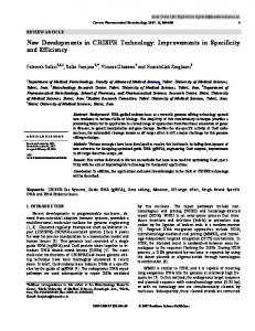
Figure 1.1: On the left, a sketch of a typical configuration for a combination crosshole and borehole-to-surface GPR experiment. Borehole separation and depth, spatial and time sampling and antennae frequency are the key parameters in such an investigation. On the right, system calibration prior to a radar survey in a field campaign. Only a few people are needed to operate a typical GPR system. depend on the experimental design of the survey, specifically the transmitter receiver locations and the central frequency/bandwidth of the source wavelet. Penetration depth is largely determined by the medium conductivity and permittivity and also by the source frequency (see 1.12-1.13). As explained in section 1.2, EM signals travel further in more resistive ground, and lower frequency signals have a greater penetration depth than higher frequency signals. It is convenient to distinguish between depth (or temporal) resolution and lateral (or azimuthal) resolution. Depth resolution refers to the Rayleigh one-quarter wavelength criterion, or the ability to distinguish between two closely spaced reflectors along a vertical line through the source-receiver midpoint. For example, in GPR it may refer to the minimum resolvable bed thickness, with reflections from its top and bottom. Depth resolution does not depend on the depth of the reflectors (scatterers) but on the pulse period relative to the two way time difference between the two reflections. The minimum distance DR that is resolvable is given by: Tv λ = , (1.17) 4 4 where T indicates the width (in time) of the signal, v is the velocity in the medium and λ is the wavelength of the GPR dominant frequency. Lateral resolution, on the other hand, indicates the ability of a GPR system to discriminate between two scatter points located a certain distance apart in the horizontal plane at a given depth below the source-receiver centre-point. This is related to the radius of the first Fresnel zone and it can be easily shown (Annan, 2002) that the minimum DR =

1.4 Applications

13

distance LR resolvable in this case is given by : r dλ (1.18) LR = 2 where and d is the depth. The ability to laterally resolve buried features therefore decreases with increasing depth. Once the radar antennae are fixed, the ability to distinguish lateral features therefore decreases with depth.

1.4

Applications

GPR finds wide applications in many different areas (Daniels, 2004;Jol, 2009). Examples include: ⊲ geological and hydro-geological investigations (mapping of bedrock topography, soil layers, water table levels, glacial structures etc); ⊲ engineering site investigations (characterization of tunnels, road pavements, railway lines, rebars, voids, etc.); ⊲ archaeological investigations (identification of tombs, rooms, artifacts, walls, buried roads etc.) and animal burrows); ⊲ utility mapping (localization of underground storage tanks, barrels, pipes etc.); ⊲ forensic investigations (detection of metallic objects, large contrast anomalies like bones or human tissue); ⊲ military operations (detection of unexploded landmines, tunnels, weapon deposits). GPR investigations can be broadly divided into two categories: Material air water sea water dry sand saturated sand clay granite ice asphalt human bones

ǫr 1 80 80 3-5 20 - 30 5 - 40 6 3.18 2-3 6 - 25

σ [mS/m] 0 0.01 4000 0.01 0.1 - 1 2 - 1000 0.01 1 0.01 0.01 25 - 200

Table 1.1: Relative permittivity ǫr and electrical conductivity σ for materials of interest in GPR investigations (modified after Knoedel et al., 1997).

1.5 Forward and Inverse GPR Problems

14

⊲ imaging reflector geometry (positions and shape) by means of back-scatter or reflection surveys, ⊲ reconstructing the dielectric permittivity (ǫ) and electric conductivity (σ) distributions in the subsurface by means of transmission tomography surveys. Most reflection surveys are conducted from the ground surface, with transmitting and receiving antennae located along linear profiles. Generally, such data are processed using migration-type algorithms borrowed from seismic imaging to obtain the structural geometry and sediment stratigraphy. This is especially true for 3D imaging, where migration is at the present time the only feasible approach. In crosshole surveys, the acquisition of GPR data entails generating EM pulses at numerous transmitter locations along one borehole and recording the responses at a large number of receiver positions along a second (or more) borehole. Data generated by a borehole transmitter antenna can also be received by antennae located at the surface (borehole-to-surface configuration). Such borehole applications significantly extend the angular coverage of the target (hence tomographic imaging ability) compared to surface surveys.

1.5

Forward and Inverse GPR Problems

The set of electrical parameters required to fully characterize the subsurface comprises the permittivity, conductivity and permeability distributions. The availability of such information allows one to theoretically solve Maxwells equations and compute the GPR response of a given model, once the antenna position, type and source current density waveform is specified. This is called the solution of the forward problem and is perfectly straightforward and stable, although it should be appreciated that for all but the most simplistic models for which analytic solutions exist, a numerical technique is required to solve the governing equation. Numerical techniques include finite-difference, finiteelement and boundary-integral approaches. For the forward problem, a unique solution is known to exist and to exhibit several continuity properties with respect to the model parameter distributions. The forward problem is then said to be well posed. The determination of the subsurface electrical parameters from the measured radar response at a finite number of source and receiver positions is known as the solution of the inverse problem. Solutions to inverse problems are most often not-unique and do not depend continuously on the input data (i.e., the measured electric and/or magnetic fields). Inverse problems are then said to be ill-posed and in order to obtain a solution it is typically necessary to impose constraints (e.g. place upper and lower bounds on permissible parameter values, require the model to be close to some preferred model, etc.). For data contaminated by noise, a unique solution seldom exists, so inverse problems are most often formulated as optimization processes. The optimization is non-linear and can be tackled using either global algorithms such as Monte Carlo search, simulated annealing and genetic algorithms (which explore the solution space) or local search algorithms that require a starting model that is subsequently refined or updated in accordance with data misfit (between the observed and computed data) and the data sensitivity functions (Greenhalgh et al., 2006). This class of inversion algorithm includes iterative full-waveform gradient-based methods (most common in GPR) or Gauss-Newton methods (common in seismic inversion). Local search algorithms are the only viable option

1.6 Ray-Based Inversion

15

for large scale inverse problems in which many parameters are needed to characterize the model. Least-squares local search algorithms such as gradient methods try to find the model (in most GPR inversions the ǫ and σ distributions) whose synthetic radar response best fits the observed data with respect to the L2 norm. Inversion however is not limited to least-squares fitting and other more robust approaches (e.g. the L1 norm) exist. A-priori knowledge can also be incorporated in the inversion process by means of damping or smoothness constraints. In the following, I give a brief introduction to ray-based and full-waveform inversion approaches.

1.6

Ray-Based Inversion

Tomographic inversions of radar data are generally based on geometrical ray theory. Conventional ray tomography can suffer from critical shortcomings associated with the inherent high frequency limit of the ray approximation, the limited angular coverage of the target (dependent on site access and apertures of the arrays), and the small number of signal attributes (first-arrival times and maximum amplitudes as indicated in Figure 1.2) employed in the inversion process. For instance, the minimum feature size resolvable by ray tomography is of the order of the first Fresnel-zone width (Williamson, 1991; Williamson and Worthington, 1993). Furthermore, theoretical considerations suggest that low-velocity (high permittivity) anomalies are by-passed by first-arriving rays and therefore are poorly imaged by ray-tracing inversion schemes. Ray tomography can be used to supply starting models for full-waveform inversion, to identify broad structures, and estimate average medium properties.

Ray-based methods Input data: - A: First-arrival time - B: Maximum first cycle amplitude

Absolute Amplitude

Bx A x

0

20

40

60 Time [ns]

80

100

120

Figure 1.2: Traveltime tomography is based on high frequency and other intrinsic ray approximations and only inverts a small fraction of the available data (i.e., the first arrival times and the first cycle maximum amplitudes). However, it is extremely direct, relatively inexpensive and provides reasonable starting models for full-waveform inversion.

1.7 Full-waveform Inversion

1.7

16

Full-waveform Inversion

To improve the limited resolution provided by travel-time methods, full-waveform inversion schemes have been developed and progressively applied. Full-waveform inversion schemes are extremely expensive in a computational sense, because they require the numerical solution of Maxwell’s equations using finite-difference or finite-element methods to obtain the synthetic electric and/or magnetic field traces to be compared with the observed traces of interest (see Figure 1.3). For non-linear inversion, this is done many times and the model is updated after each iteration. The potential improvement in resolution offered by waveform √ methods, under the most ideal conditions, has been estimated to be of the order of N λ , where Nλ is the average number of wavelengths over the source and receiver paths (Pratt and Shipp, 1999). Early versions of full-waveform EM inversion were based on the Born approximation of weak scattering (i.e., for low contrast targets), thus neglecting secondary interactions between obstacles (Chew and Wang, 1990; Wang and Rao, 2006). State-of-the-art microwave imaging was described by Dubois et al. (2009), Rubaek et al. (2009) and Soldovieri (2010). Despite the elegance of these inversion schemes, their applicability to GPR is limited. It is in fact often assumed in microwave imaging that the transmitters and receivers are polarised in the 2D medium-invariant transverse or y-direction, such that the EM equations (transverse electric or TE case) for a line source simplify considerably to scalar wave equations involving a single E-field component (Ey ). This is only applicable in GPR for surface recording in which the antennae are directed perpendicular (y direction) to the profile (x) direction and the geology is two dimensional. For antennae oriented in the saggital plane (i.e., for a TM mode) or for 3D media, such equations cannot be

Waveform methods - Input data:

Absolute Amplitude

Significant parts of wavefields - Inversion based on Maxwell eq.

0

20

40

60 Time [ns]

80

100

120

Figure 1.3: Full-waveform inversion requires the numerical solution of Maxwell’s equations and inverts the entire wavefields (or portions of them). It can theoretically provide very high resolution images, but it is significantly more expensive than traveltime tomography and more prone to local minimum trapping.

1.7 Full-waveform Inversion

17

used, thus seriously limiting such approach as for more general GPR applications. Ernst et al. (2007a) and Kuroda et al. (2007a) were among the first researchers to tackle theoretically crosshole full-waveform GPR inversion as a non-linear iterative problem, providing a general solution applicable to any mode and model dimension, even if applications were limited to two dimensional problems. Both inversion schemes were based on a gradient method and operate in the time domain. To account for the large sensitivities differences between permittivity and conductivity, Kuroda et al. (2007a) inverted only for the relative permittivity ǫ. Ernst et al. (2007a), on the other hand, used a stepped (cascaded) inversion scheme, whereby the ǫ distribution was first (b) Ray-Based Inversion

(c) Full-waveform Inversion

(d) Real Model

(e) Ray-Based Inversion

(f) Full-waveform Inversion

Conductivity

Permittivity

(a) Real Model

Figure 1.4: Advanced full-waveform algorithms such as the one proposed by Ernst et al. (2007a) can provide very good reconstruction of complex models. (a) and (d) show the highly heterogeneous, quasi-layered permittivity and conductivity distributions that are used to generate sets of traces corresponding to transmitter and receiver positions indicated by the crosses and circles through (a)-(f). (b)-(c) and (e)-(f) show permittivity and conductivity reconstructions resulting from the applications of ray-based and fullwaveform inversions. Whereas (b) and (e) only recover the very coarse structures of (a) and (d), (c) and (f) provide high resolution images.

1.8 Computational Electrodynamics

18

updated while the σ distribution was held fixed, and then the σ values were updated holding the ǫr values fixed. In Figure 1.4 an inversion result obtained by employing the inversion algorithm of Ernst et al. (2007a) is presented. Ernst et al. (2007b) successfully applied their technique to observed data from two field sites. Full-waveform inversion can also (in principle) be performed by employing GaussNewton or full-Newton algorithms. These methods are known to provide faster and better convergence, but are extremely expensive from a computational point of view because they require explicit calculation of the Jacobian matrix and inversion and multiplication of very large matrices. To date, they have not been applied to GPR waveform inversion.

1.8

Computational Electrodynamics

Sophisticated inversion schemes such as full-waveform inversion require multiple simulations of electromagnetic fields. In this section, I give a very brief review of some of the most widely used forward solvers, together with a few historical details. The interested reader is referred to Taflove and Hagness (2005) for more details about the history of computational electrodynamics and current applications. Historically, the motivation to compute solutions for EM wave-propagation problems was mainly driven by military concerns during the Second World War and the Cold War eras. Until the late 60s, most approaches involved either closed form analytical solutions or high-frequency asymptotic methods and integral equation approaches (e.g., boundary element method). However, the idealized assumptions or the huge memory required by these and frequency-domain algorithms constituted a serious limitations with respect to their applicability at the time. Since the seminal work by Yee (1966), finite-difference time-domain (FDTD) has emerged as the most popular and flexible computational electromagnetic technique. The most notable steps in the developments of FDTD include the following aspects: ⊲ numerical stability criteria; ⊲ absorbing boundary conditions; ⊲ numerical dispersion quantification. In the context of numerical modelling, the solution of a discretized problem is said to be stable if it produces a bounded result given a bounded input. A solution is said to be unstable if it produces an unbounded result given a bounded input (Taflove and Hagness, 2005). Stability criteria associated with Yee’s algorithm were first introduced by Taflove and Brodwin (1975), who found that a certain relationship between time and spatial sampling has to exist in order to prevent exponential growth of the amplitudes of the field with increasing time. One of the most critical aspects of FDTD modelling has been the accurate simulation of wave propagation in unbounded media. The need to keep the modelled region as small as possible in order to minimize the computational burden (memory and run time) in fact conflicts with the problems arising at model boundaries (i.e., spurious back reflections into the simulation region of interest). The first numerically stable second-order accurate absorbing boundary condition for Yee’s grid was introduced by Mur (1981), while highly

1.9 Thesis Objectives and Outline

19

effective perfectly matched layers (PML) were later developed by Berenger (1994). They were subsequently developed in the elegant and general framework of complex coordinate stretching by Chew and Weedon (1994). Numerical dispersion of waves concerns the phenomenon of non-physical dependence of phase velocity on frequency and direction of propagation. It arises when the spatial grid interval is not small enough relative to the shortest wavelength in the model to be simulated. A detailed relationship based upon complex wavenumbers of numerical dispersion, along with a guideline about the choice of spatial grid to avoid it, is given by Schneider and Wagner (1999); a minimum of ten grid samples for the shortest wavelength is recommended to avoid noticeable numerical dispersion. Despite the intrinsic limitation of FD methods for handling topography compared to some other methods (i.e., finite elements) and the complexity involved when introducing denser meshes (e.g., as in the simulation of antennae), the great flexibility and the relatively low computational costs of FDTD have extended the interest in computational electrodynamics well beyond military applications. Nowadays, FDTD schemes are used to study a variety of problems, ranging from earth scale geosciences to microwave biomedical imaging, with hundreds of FDTD related papers published every year.

1.9

Thesis Objectives and Outline

The primary objective of this thesis was to improve the inversion of full-waveform GPR data through theoretical and algorithmic developments. I restricted myself to 2D models, an FDTD modeling scheme and a gradient-based inversion approach. Specifically the aims of my research were to: 1. utilise the full radar traces (including reflected and diffracted signals) , not just the first few cycles (direct transmitted pulse) as in most previous schemes; 2. take into account the vectorial nature of the E field from a directed (dipole) source, for computing the gradients; 3. devise a scheme that was capable of combining crosshole data (with antenna polarized in the vertical direction) with borehole-to-surface data (having the surface antennae polarized in the horizontal direction); 4. perform a simultaneous update of the permittivity and conductivity during the inversion, rather than a cascaded or sequential approach in which one set of parameters is held fixed while the others are updated, and then conversely holding that set fixed while the other parameters are updated; 5. reduce the degree of non-linearity of the inverse problem, and preclude local minimum trapping through a combined time-frequency-domain approach; 6. assess the reliability of the inverted image through formal sensitivity and resolution analyses. In the first stage of my Ph.D. (Chapter 2) I developed a new full-waveform timedomain inversion algorithm incorporating items (1)-(4) above , to improve the imaging


20

capability of full-waveform inversion. The novelty of such an approach did not only rely on the new algorithm but also on my original full-wavefield vectorial formalism used to express the governing equations. This innovation was not intended to be just more compact, but due to the relatively simple formula derived there, it was used to express the gradient of the cost function and the sensitivity kernels. The necessity to include all components of the electric field in the definition of the updating direction, as opposed to the previous scalar-based approaches, was readily apparent. This then enabled a full-vector treatment of the problem. This research was published in the journal IEEE Transactions on Geosciences and Remote Sensing, vol. 48, pp:3391-3407 (Meles et al., 2010). In the second stage of my Ph.D. (Chapter 3) I presented a different algorithm (item 5 above) for the inversion of full-waveform GPR data (Meles et al., 2011). The new scheme was designed to tame the non-linearity issue that afflicts inverse scattering problems, especially in high contrast media. Despite having established a solid imaging scheme in the context of weak scattering, several numerical examples showed that the scheme presented in Meles et al. (2010) was not able to invert datasets involving large misfits between the starting and the true model. By means of theoretical considerations and a few extremely convincing thought-experiments, a very simple yet effective approach to inversion was proposed to overcome these limitations. Owing to the clarity provided by the mathematical formalism I had introduced in my first paper, it was relatively easy to propose a new inversion scheme that combined the benefits of both the time and the frequency domain. The technique uses a progressive expansion of the bandwidth as iterations proceed, starting at low frequency. The new scheme has been compared to our previous state-of-the-art scheme. A large number of synthetic results clearly demonstrated that the new scheme can markedly improve the quality of the inversion results, largely avoiding local minima and strong artifacts in the permittivity and conductivity images. This research was published in the Journal of Applied Geophysics, vol. 73, pp:174-186 (Meles et al., 2011). In the last part of my Ph.D. research (Chapter 4), I tackled item (6) above to appraise the fidelity and credibility of a tomogram, which is a critical yet somewhat ignored aspect of any inversion procedure. The reliability and resolution of the final image need to be assessed. Most often, simple convergence in the data space (i.e., the matching of the observed and the synthetic radar traces) is the only criterion used to appraise the goodness of the final result. Particularly in real data inversions, for which the true permittivity and conductivity distributions are unknown, this can lead to severe misinterpretation, because convergence in the data space does not guarantee convergence in the model space. A better indication of the reliability of an inverted model for a given GPR recording configuration could be obtained by means of a formal resolution analysis. This requires knowledge of the Fréchet derivatives or sensitivity functions. However, gradient-based methods do not involve explicit computation of the sensitivity (or Jacobian) matrix. The new sensitivity formulation developed as part of this research has also opened up the possibility of performing Gauss-Newton inversion, previously not possible in time-domain GPR imaging. Owing to the clarity provided by the formalism I introduced in Meles et al. (2010), a computationally feasible expression of the Jacobian was derived via an adjoint method.


21

The availability of the Jacobian matrix not only provides an assessment of the sensitivities of the data, but also allows the computation of the pseudo-Hessian matrix and the model resolution matrix. The normalized eigenvalue spectrum of the pseudo-Hessian matrix is shown to provide an estimate of the well-resolved portion of the model space versus the null space. Therefore, the analysis of model resolution and the eigenvalue distribution, both provided by the sensitivity kernels, defines a methodology for the interpretation and appraisal of an inversion result. This work has been submitted for publication in the journal IEEE Transactions on Geoscience and Remote Sensing. Chapter 5 of this thesis is a published account of a field data GPR example from Switzerland which was inverted using my new vectorial and simultaneous updating algorithm (Chapter 2). The paper, co-authored by me and published in Near Surface Geophysics vol. 8, pp:635-649 (Klotzsche et al., 2010), involved crosshole radar imaging to characterize a gravel aquifer in an area of strong hydrological interest. My main contribution was to provide the code, advise on its use and to help interpret the inverted images. Chapter 6 is a conclusions and outlook chapter that summarises the main findings reported in chapters 2-5. It identifies a number of promising follow-up topics that are deserving of further research. The outlook includes TE and TM mode inversion, timedomain Gauss-Newton and full Newton GPR inversion, use of multiple step lengths and optimal step lengths by parabolic interpolation, emphasizing later portions of the radargram and compensation for radiation pattern effects on sensitivities, and 3D /2.5D inversion of real data. Four appendices are included with this thesis and they deal with more specialised technical aspects of GPR inversion. They are: ⊲ C-1 The effect of non-linearity on the forward problem; ⊲ C-2 Grid dispersion in FDTD modeling; ⊲ C-3 Hard and soft sources in FDTD modeling; ⊲ C-4 SVD resolution and choice of the damping factor.

22

Chapter 2 A New Vector Waveform Inversion Algorithm for Simultaneous Updating of Conductivity and Permittivity Parameters From Combination Crosshole/Borehole-to-Surface GPR Data Giovanni Angelo Meles, Jan Van der Kruk, Stewart A. Greenhalgh, Jacques R. Ernst, Hansruedi Maurer, and Alan G. Green Published in: IEEE Transactions on Geoscience and Remote Sensing, 48, 2010, 3391-3407

Abstract We have developed a new, full-waveform GPR multi-component inversion scheme for imaging the shallow subsurface using arbitrary recording configurations. It yields significantly higher resolution images than conventional tomographic techniques based on first-arrival times and pulse amplitudes. The inversion is formulated as a non-linear leastsquares problem in which the misfit between observed and modelled data is minimized. The full-waveform modelling is implemented by means of a finite-difference time-domain solution of Maxwell’s equations. We derive here an iterative gradient method in which the steepest descent direction, used to update iteratively the permittivity and conductivity distributions in an optimal way, is found by cross-correlating the forward vector wavefield and the backward-propagated residual wavefield. The formulation of the solution is given in a very general, albeit compact and elegant fashion. Each iteration step of our inversion scheme requires several calculations of propagating wavefields. Novel features of the scheme compared to previous full-waveform GPR inversions are that (i) the permittivity and conductivity distributions are updated simultaneously (rather than consecutively) at each iterative step using improved gradient and step length formulations,

2.1 Introduction

23

(ii) the scheme is able to exploit the full vector wavefield, and consequently (iii) various data sets/survey types (e.g., crosshole, borehole-to-surface) can be individually or jointly inverted. Several synthetic examples involving both homogeneous and layered stochastic background models with embedded anomalous inclusions demonstrate the superiority of the new scheme over previous approaches.

2.1

Introduction

Ground-penetrating radar (GPR) is a non-invasive technique used to investigate properties of the shallow subsurface. It uses high frequency (20-1000 MHz) electromagnetic (EM) waves that interact with underground geological obstacles and discontinuities. The dominant wavelengths are in the range of 5-0.1 m for commonly occurring earth materials. The GPR method can be used in either a transmission or a reflection mode to provide tomographic images of permittivity (ε) and conductivity (σ) distributions. Applications are diverse, including civil engineering site investigations (Grandjean et al., 2000; Kao et al., 2007; Soldovieri et al., 2007), landmine detection (Ho et al., 2008), environmental and hydrogeological studies (Knight, 2001; Binley et al., 2001, 2002a; Tronicke et al., 2004; Looms et al., 2008; Linde et al., 2006), agricultural assessment (Hubbard et al., 2005; Weihermuller et al., 2007; Lambot et al., 2004; Huisman et al., 2003), and archaeological investigations (Carcione, 1996; Baker et al., 1997), where knowledge on bedrock, soils, soil water content, groundwater, and even ice is required. The resolving power and depth range of GPR are limited by the frequency content of the pulse and the electrical conductivity of the ground: high frequency electromagnetic pulses give better resolution but are more rapidly attenuated, so the depth of penetration is less. Most applications of GPR are conducted from the ground surface, with transmitting and receiving antennae located along linear profiles. Mostly, such data are processed in a migration-style sense using the Born approximation, to obtain the structure and medium properties of the subsurface (Crocco and Soldovieri, 2003; Oden et al., 2007; Pettinelli et al., 2009). This is especially true for 3D imaging where migration is at the present time the only feasible approach (Streich et al., 2007). In crosshole surveys, acquisition of GPR data entails generating EM pulses at numerous transmitter locations along one borehole and recording the responses at a large number of receiver positions along a second borehole. Data generated by a borehole transmitter antenna can also be received by antennae located at the surface (borehole-to-surface configuration). Such borehole applications significantly extend the depth of coverage compared to surface surveys. Tomographic inversions of radar data are generally based on geometrical ray theory. Conventional ray tomography can suffer from critical shortcomings associated with the inherent high frequency limit of the ray approximation, the limited angular coverage of the target, and the small number of signal attributes (first-arrival times, maximum amplitudes) employed in the inversion process. For instance, the minimum feature size resolvable by ray tomography is of the order of the first Fresnel-zone width (Williamson, 1991; Williamson and Worthington, 1993). Furthermore, theoretical considerations suggest that low-velocity (high permittivity) anomalies are by-passed by first-arriving rays and therefore are poorly imaged by ray-tracing inversion schemes (Flecha et al., 2004). To improve the limited resolution provided by travel-time methods, full-waveform inver-

2.2 Forward Problem

24

sion schemes can be applied. The potential improvement in resolution that can be gained by applying waveform √ methods, under the most ideal conditions, has been estimated to be of the order of N λ , where Nλ is the number of wavelengths between the sources and receivers (Pratt and Shipp, 1999). The aim of inversion is to find the model (in GPR inversion, the permittivity and conductivity distributions) whose synthetic radar response best matches the observed data. In the case of full-waveform inversion, the data are entire wavelets or entire waveforms and not, as for travel-time tomography, only a small fraction of the information collected. Full-waveform inversion is fairly advanced in exploration seismics (e.g. Mora, 1987; Tarantola, 1986, 1984a,b; Reiter and Rodi, 1996; Gauthier et al., 1986; Tarantola and Valette, 1982; Devaney, 1984; Wu and Toksoz, 1987) whereas in GPR it is still under development (Gustafsson and He, 2000a; Kuroda et al., 2007a,b; Ernst et al., 2007a,b; Fhager and Persson, 2007). Previous GPR waveform inversion schemes were based on some simplifying assumptions: (a) originally only media with homogeneous conductivity distributions were investigated (Kuroda et al., 2007a,b), (b) most algorithms were based on a scalar approximation and only a stepped (cascaded) updating of the permittivity and conductivity distributions was attempted (Ernst et al., 2007a,b), or, (c) if simultaneous updating of permittivity and conductivity was attempted, the inversion results were overly sensitive to the choice of several empirical scaling factors (Fhager and Persson, 2007). In this paper, a new inversion scheme based on both a vectorial approach and simultaneous updating of the permittivity and conductivity distributions is presented. In the following, the general form of the new full-waveform inversion scheme is derived and described. The new inversion scheme is compared with the recently developed algorithm of Ernst et al. (2007a), which is based on a scalar approximation of the electric field and a stepped (cascaded) updating of parameters. The improvements that result from the new developments, especially those resulting from jointly inverting crosshole and borehole-to-surface data together, are illustrated by means of several synthetic examples.

2.2

Forward Problem

The minimum set of electrical parameters required to characterize completely the subsurface comprises the permittivity, conductivity and permeability distributions. Throughout the rest of this paper, permeability is assumed to be constant and equal to µ0 . Maxwell’s equations can then be written in a compact form as follows: s s E J M(ε, σ) = . (2.1) s H 0 Here, Es and Hs are the electric and magnetic fields generated by the current density source vector Js . The superscript ’s’ stands for a particular source. M(ε, σ) is a linear operator that represents Maxwell’s equations, locally defined at any point of time t and

2.2 Forward Problem

25

space x as:

−ε(x)∂t − σ(x) ∇× ∇× µ0 ∂t

Es (x, t) Hs (x, t)

=

Js (x, t) 0

,

(2.2)

where ε(x) and σ(x) are the permittivity and conductivity distributions, respectively. The field quantities are vectorial functions of space and time, while the medium properties are scalar functions of position. The vector quantities Es , Hs , and Js do not stand for the fields at a specific space-time position, but comprise the whole space-time domain of interest, viz. Es = {Es (x, t), ∀t ∈ T , ∀x ∈ V } .

(2.3)

We present below an algorithm for the inversion of electric wavefields, which when using our compact wavefield vector notation results in a much simpler and clearer derivation of the whole inversion scheme compared to previous approaches (Gustafsson and He, 2000a; Kuroda et al., 2007a; Ernst et al., 2007a). We have attempted to give a full, general and self-contained wavefield treatment of the problem. Important intermediate steps are sometimes missing in the earlier literature, or the formulations are overly complicated, so the reader could miss some of the essential points. Eliminating Hs from (2.1), because in the following only the electric field is investigated, results in the simple formulation: ˆ s, Es = GJ

(2.4)

ˆ is the Green’s operator of M. Later on we will use (2.4) as a formal reprewhere G sentation of a solution of a forward problem. The explicit representation of (2.4) for a specific time-space point (x, t) is given by: Es (x, t) =

Z

dV (x′ )

ZT

dt ′ G(x, t, x′ , t ′ )Js (x′ , t ′ ),

(2.5)

0

V

where Es (x, t) is the electric field at (x, t) generated by the source Js and G(x, t, x′ , t ′ ) is the Green’s tensor of our problem that acts on the source term Js (x′ , t ′ ). We can also express each component of the electric field explicitly with the following Cartesian tensor (or index) notation: Eis (x, t)

=

Z

V

′

dV (x )

ZT

dt ′ Gik (x, t, x′ , t ′ )Jks (x′ , t ′ ),

(2.6)

0

i and k = x, y, z; where Eis (x, t) are the individual components of the electric field, and Gik (x, t, x′ , t ′ ) and Jks (x′ , t ′ ) are the components of the Green’s tensor and of the source term, respectively. Summation is implied in the above equation through repetition of subscript k. We will primarily use vector notation throughout our formulation, but it is convenient to return

2.3 Inverse Problem

26

to the tensor form in Appendix A.1 for examining the transpose of G and utilizing the reciprocity relation. In the remaining part of this paper, we indicate with a bold font, E, an entire wavefields, with normal font, E(x, t) a vector function at a specific point, and with an italic font, Ei (x, t) a single component of a vector function at a specific point. [Es ]d,τ is the projection of Es on detector (receiver) position d at observation time τ . As an explicit example, [Es ]d,τ is the vectorial wavefield Es at receiver position d and observation time τ , and is 0 elsewhere.

2.3

Inverse Problem

There are various approaches to the geophysical inverse problem (Greenhalgh et al., 2006). Our full-waveform tomographic inversion scheme involves finding the spatial distributions of ε and σ that minimize the squared norm S(ε, σ) of the difference between the simulated and the observed traces. Using our formalism, this can be written as: S(ε, σ) =

1X s [E (ε, σ) − Esobs ]Td,τ 2 s,d,τ

· δ(x − xd , t − τ ) [Es (ε, σ) − Esobs ]d,τ ,

(2.7)

where Es (ε, σ) and Esobs are the synthetic and observed data, respectively, T indicates the transpose operator and the sums are over sources s, receivers d , and observation times τ . We minimize the functional (2.7) using a gradient-type scheme based on an algorithm introduced by Polak and Ribiere (1969) which can be distilled into the following steps 1. Select an initial model ε = εini and σ = σini (these can be defined by the results of prior ray tomographic inversions of the first-arrival times and maximum first-cycle amplitudes (Luo and Schuster, 1991; Holliger et al., 2001); 2. Compute the synthetic wavefields Es (ε, σ) using the initial model parameters; 3. Compute the update directions (the gradients in a steepest descent method) ∇Sε and ∇Sσ ; 4. Compute the step lengths ζε and ζσ ; 5. Update the model parameters using the steepest descent equations εupd = ε − ζε ∇Sε , σupd = σ − ζσ ∇Sσ ; 6. Set ε = εupd and σ = σupd and repeat actions 2 to 6 until convergence is achieved or until a specified number of iterations is reached. We next explain the linearization of the forward problem and the sensitivity operator, as well as how the gradients and the step lengths are determined. Many details on the inversion algorithm, including the gradients, step-lengths and the kernel function are provided in Appendix A.2.

2.3.1 Linearization of the Forward Problem

2.3.1

27

Linearization of the Forward Problem

The misfit function (2.7) depends on the synthetic electric field, which is a function of the permittivity and conductivity distributions. To find the gradient of the misfit function with respect to these parameters, we need to deal with a first order approximation of the electric field with respect to these values, i.e. to linearize the solution of the forward problem. Similar to (2.1), we can write Maxwell’s equations for a perturbed system as: s s E + δEs J M(ε + δε, σ + δσ) = . (2.8) s s H + δH 0 Subtracting (2.1) from (2.8) we obtain s δEs P M(ε, σ) = . s δH 0

(2.9)

This expression contains the same operator M as (2.1) and the source term, Ps , now given by Ps = ∂t Es δε + Es δσ, (2.10) is a function of the un-perturbed synthetic electric field in the space domain. We next substitute (2.9) into (2.4) and obtain ˆ t Es δε + Es δσ). δEs = G(∂

(2.11)

The operator Ls that linearizes the forward problem with respect to small perturbations in the permittivity and conductivity values is defined as follows: s s δε s s s . (2.12) E (ε + δε, σ + δσ) − E (ε, σ) = δE = Lε Lσ δσ Comparing (2.12) and (2.11), and expressing explicitly the kernel of Ls (see Appendix A.2) allows us to express the individual columns of Ls as follows: ˆ − x′ )∂t Es , Lsε (x′ ) = Gδ(x

(2.13)

ˆ − x′ )Es . Lsσ (x′ ) = Gδ(x

(2.14)

The direct computation of the components of the sensitivity operator Ls would require as many solutions of the forward problem as there are model parameters. In any case, we will show in the next section that we are not directly interested in the sensitivity operator, but only in its application to the residual, which requires just one solution of the forward problem. As the misfit function (2.7) does not consider the whole space-time domain of definition of the wavefields, in the remaining part of the paper we will be interested in the operator Fs that linearizes the electric field at all the receivers and observation time combinations for each source: X s s δε s , (2.15) [δE ]d,τ = Fε Fσ δσ s,d,τ

2.3.2 The Gradients of the Misfit Function

28

where [δEs ]d,τ = [Es (ε + δε, σ + δσ) − Es (ε, σ)]d,τ

(2.16)

For the operator Fs the columns are not as simply defined as for Ls . In the following we will still be able to use, without any additional approximation, the simpler form of Ls instead of Fs for the computation of the gradient. s s Note that L and that the projection of therange of F is a subset of the range of δε s s δε Lε Lσ . on the range of Fs equals Fsε Fsσ δσ δσ

2.3.2

The Gradients of the Misfit Function

We have introduced the cost or objective function in the following form: S(ε, σ) =

1X s [E (ε, σ) − Esobs ]Td,τ 2 s,d,τ

· δ(x − xd , t − τ ) [Es (ε, σ) − Esobs ]d,τ ,

(2.17)

As the gradient of the misfit function is defined by means of a first order approximation, viz δε T + O(δε2 , δσ 2 ), (2.18) S(ε + δε, σ + δσ) = S(ε, σ) + ∇S δσ using the same linearization as in (2.15), it is equivalent to: X T ∇S = Fs [∆Es ]d,τ ,

(2.19)

s,d,τ

where we have introduced the following notation for the residual wavefield: [∆Es ]d,τ = δ(x − xd , t − τ ) [Es (ε, σ) − Esobs ]d,τ .

(2.20)

. Due to the properties of Ls and Fs as described at the end of section 2.3.1, it follows that: Fs T [∆Es ]d,τ = Ls T [∆Es ]d,τ . (2.21) The gradients are then found by applying the transpose of Ls to the residual. More precisely, the single spatial components of the gradients are obtained by performing an inner product of the individual columns of Ls and the residual wavefield. For this reason, we have derived earlier the explicit expressions for the columns of Ls (2.13 and 2.14). Using the results summarized in (2.13) and (2.14) allows us to write the gradients as:

∇Sε (x′ ) ∇Sσ (x′ )

X (δ(x − x′ )∂t Es )T G ˆ T [∆Es ] d,τ . = s T ˆT s ′ (δ(x − x )E ) G [∆E ] s,d,τ

(2.22)

d,τ

Since the columns of the sensitivity operator are the solution of a forward problem, we can leave the term containing the forward solution Es on the left side and apply the transpose of the Green’s operator to the residual. This avoids us having to perform direct

2.3.3 The Step-Lengths

29

computation of the sensitivity operator, as foreshadowed in section (2.3.1). The above expressions are entirely general, allowing the inversion of various data sets (entailing any combination of source and receiver orientation, e.g. crosshole, borehole-to-surface). After some straightforward manipulations, we can express (2.22) as

∇Sε (x′ ) ∇Sσ (x′ )

X (δ(x − x′ )∂t Es )T G ˆ T Rs , = ′ T ˆT s (δ(x − x )E ) G R s s

where the generalized residual wavefield Rs is given by XX Rs = [∆Es ]d,τ . d

(2.23)

(2.24)

τ

ˆ T Rs In (2.23), Es indicates the solution of Maxwell’s equation in the medium, whereas G can be interpreted as a backward propagated vectorial field in the same medium (for details, see Appendix A.1). The simpler formula given by (2.23) shows that the gradient is found by summing the 3-component inner products of the forward vectorial propagated field and the backward residual vectorial propagated vectorial field over all the sources. The inner product involves an integration over the whole spatial-time domain of Es and ˆ T Rs . The presence of spatial delta functions δ(x − x′ ) corresponding to the spatial G components of the gradients ∇Sε (x′ ) and ∇Sσ (x′ ) reduces the inner product to a zero-lag cross-correlation in time (see Appendix A.1).

2.3.3

The Step-Lengths

Once the gradients are found, step-lengths are required to update the whole permittivityconductivity model. Theoretically, the dielectric permittivities and electrical conductivities should be updated according to: ∇Sε ε εupd , (2.25) −ζ · = ∇Sσ σ σupd An optimal step-length ζ can be found by following the approach introduced by Pica et al. (1990), which involves searching for a minimum of the objective function along the direction of the gradient: S(ε + ζ∇Sε , σ + ζ∇Sσ ).

(2.26)

The function in (2.26) has just one independent variable (i.e., the step-length ζ), whereas ε, σ, ∇Sε , and ∇Sσ are fixed. The minimum is achieved simply by setting to zero the first derivative ∂S(ε + ζ∇Sε , σ + ζ∇Sσ ) = 0. (2.27) ∂ζ According to Pica et al. (1990) the critical point occurs at the value given by equation: ζ=κ

P

[δEskǫσ ]Td,τ δ(x − xd , t − τ ) [Es (ε, σ) − Esobs ]d,τ . P T s s ] ] δ(x − x , t − τ ) [δE [δE d kǫσ d,τ kǫσ d,τ s,d,τ

s,d,τ

(2.28)


30

where δEskǫσ = Es (ε + κ∇Sε , σ + κ∇Sσ ) − Es (ε, σ) has been introduced for display purposes. Here, Es (ε, σ) is the synthetic wavefield for the model parameter estimates (ε, σ), κ is an empirically established small number (see Appendix A.3 for guidelines on how to choose such numbers), and Es (ε + κ∇Sε , σ + κ∇Sσ ) is the synthetic wavefield computed for perturbed permittivities and conductivities in the respective gradient direction (this process requires an additional FDTD simulation). Large differences between the permittivity and the conductivity sensitivities can cause this simultaneous inversion to fail for complex models. We quantified these differences by means of three numerical experiments which analysed the differences between radargrams generated for a specific model (e.g., model 2 in section (2.5)) and the same model perturbed in three different ways: ⊲ Combined permittivity/conductivity perturbations (E(ε + κ∇Sε , σ + κ∇Sσ ) − E(ε, σ)),

10 times Permittivity update

a) b)

(a)

(b)

Model εr0 Model σ 0

Model εr 0 Model σ 0

Calculate Misfit Calculate Gradient

FDTD

+ r

FDTD

Calculate Misfit

FDTD

+ b)

Calculate Gradients

r,

FDTD

+ c) d)

r Step Length

Update Model

a) b)

+

FDTD

c)

r

Step Length Step Length

2FTDTs

3 FDTDs

d)

Model εr 10 Model σ 0

10 times Conductivity update

a)

Calculate Misfit

FDTD

Calculate Gradient

FDTD

+

Update Model

4FDTDs

Model εr 10 Model σ10 After 10 iterations: 4 FDTDs x 10 = 40 FDTDs

+

c)

Step Length

FDTD

d)

Update Model

3 FDTDs

Model εr10 Model σ10 After 10 iterations: (3 + 3) FDTDs x 10 = 60 FDTDs

Figure 2.1: Flow diagrams of the cascaded (a) and the simultaneous (b) inversion algorithms.


31

⊲ Pure conductivity perturbation (E(ε, σ + κ∇Sσ ) − E(ε, σ)), ⊲ Pure permittivity perturbation (E(ε + κ∇Sε , σ) − E(ε, σ)). These tests showed that there is a two order of magnitude difference between the conductivity-only variation and the other two, which look very similar. The step-length is therefore determined by the permittivity gradient in such a scheme. Ernst et al. (2007a) proposed a stepped or cascaded inversion that involves inverting for the permittivities while keeping the conductivities fixed (constant) for a certain number of iterations and then analogously inverting for the conductivities keeping the permittivities fixed. In order to minimize the effects of conductivity anomalies during the permittivity inversions, a normalized version of the data residual was exploited, by dividing through by the energy in the modelled traces while the ordinary residual was used for the conductivity inversions. The reader is referred to Ernst et al. (2007a) for details. In contrast, Tarantola (2004) suggests updating different types of model parameters according to different step-lengths. In the GPR case, this becomes εupd = ε − ζε · ∇Sε , (2.29) and

σupd

=

σ

− ζσ ·

∇Sσ

.

(2.30)

We present here a quasi-simultaneous inversion that updates the permittivities and the conductivities at each iteration by searching for critical points separately along the ∇Sε and ∇Sσ directions. S(ε + ζε ∇Sε , σ). (2.31) S(ε, σ + ζσ ∇Sσ ).

(2.32)

The two critical points of (2.31) and (2.32) occur at the values given by the equations: [δEsκǫ ]Td,τ δ(x − xd , t − τ ) [Es (ε, σ) − Esobs )]d,τ , P s s T s,d,τ [δEκǫ ]d,τ δ(x − xd , t − τ ) [δEκǫ ]d,τ

ζε = κε

P

ζσ = κσ

P

and

s,d,τ

[δEsκσ ]Td,τ δ(x − xd , t − τ ) [Es (ε, σ) − Esobs )]d,τ . P s s T ] ] δ(x − x , t − τ ) [δE [δE d κσ κσ d,τ d,τ s,d,τ

s,d,τ

(2.33)

(2.34)

where κε and κσ are two different small stabilizing numbers and for display purposes the quantities δEsκǫ = E(ε + κε ∇Sε , σ) − Es (ε, σ) and δEsκσ = Es (ε, σ + κσ ∇Sσ ) − Es (ε, σ) have been introduced. Note that the small stabilizers κε and κσ in (2.33) and (2.34) must be chosen carefully between upper and lower limits (see Appendix A.3 for details). These stabilizing numbers may need to be updated during the inversion process as a consequence of the variations in the gradient amplitudes (Pica et al., 1990). In our numerical experiments, values of κε = 10−5 and κσ between 1 and 25 were found appropriate. Although this newly introduced process requires an additional forward model calculation, the simultaneous nature of the process results in a reduction in the total

2.3.4 Different Parameterizations of the Physical System

32

number of required FDTD calculations, because it updates both the permittivity and conductivity distributions at each iteration (see Figure 2.1). Our full-waveform inversion scheme requires the forward problem to be solved four times per iteration at each transmitter location: once to evaluate the synthetic data, once to compute the update in both gradient directions, and twice to determine the step lengths. By comparison in Ernst et al. (2007a) different residuals were used such that the permittivity and conductivity gradients could not be computed with a single forward model calculation and six forward solutions were needed. In addition, while the cascaded scheme requires the user to select or choose the number of permittivity/conductivity iterations to be executed before updating the conductivity/permittivity, the simultaneous inversion does not. As a result, the implementation of the simultaneous inversion scheme is simpler. The differences between the algorithm employed by Ernst et al. (2007a) and the new inversion scheme are highlighted in the processing flow chart of Figure 2.1. This diagram is for 10 iterations, but it can be extended to any number. It involves 10 simultaneous updates of permittivity and conductivity, requiring 40 forward model computations. This can be compared to 10 permittivity updates followed by 10 conductivity updates with the cascaded scheme, involving 60 forward model runs. The solutions are not the same in each case. Note that the simultaneous scheme only involves 2/3 the computational effort.

2.3.4

Different Parameterizations of the Physical System

We have presented here the derivation of the inversion algorithm based on the natural parameters ε, σ and µ0 . Different parametrizations (i.e., changes of coordinates in the model space) can, however, be easily implemented. A logarithmic representation for the permittivity and the conductivity is normally used: ε(x) εˆ(x) = log , (2.35) ε0 σ(x) σˆ (x) = log , (2.36) σ0 where ε0 is the vacuum permittivity and σ0 is an arbitrary conductivity value, in our case 1 S/m. The choice of logarithmically scaled parameters is especially important for the inversion, because it conveys to the model space the structure of a linear space (Tarantola, 2004). In addition, this parameterization ensures positive values of permittivity and conductivity and allows compression of model values to accommodate a much wider range (Kuroda et al., 2007a). A change of model representation for the inversion process affects just the formula of the gradient directions. First, we introduce a new representation for the objective function S(ε(ˆ ε), σ(ˆ σ )) = S ′ (ˆ ε, σ ˆ ),

(2.37)

and then we express the new gradients ∇Sεˆ′ and ∇Sσˆ′ as functions of ∇Sε and ∇Sσ , whose values are expressed in (2.23). ∂S ′ ∂S ∂ε = ∂ εˆ ∂ε ∂ εˆ

and

∂S ′ ∂S ∂σ = . ∂ σˆ ∂σ ∂ σˆ

(2.38)

2.4 Implementation

Using the definition given by (2.35) and (2.36) we find ∇Sεˆ′ (x′ ) ε(x′ )∇Sε (x′ ) = . ∇Sσˆ′ (x′ ) σ(x′ )∇Sσ (x′ )

2.4

33

(2.39)

Implementation

The theory presented so far is entirely general and can be applied to 3D or 2D problems. However, the computing resources needed to simulate many multiple forward calculations in 3D using a finite-difference time-domain (FDTD) scheme (Yee, 1966), are prohibitively expensive at the present time. We therefore test our inversion scheme in laterally-invariant (2D) media with line sources (in y direction) in a Cartesian coordinate frame. Assuming no medium property variations in the y direction, the six components of the EM field are decoupled into two independent sets of equations (Taflove and Hagness, 2005). We can then solve for just one of these sets. For a borehole configuration, we solve Maxwell’s equations for the TEy mode, (i.e. the mode whose electric field is always transverse to the y direction (Balanis, 1989) which involves the following field components: (Ex , Ez and Hy ). Note that theoretically the algorithm can deal with all source and receiver combinations at the same time. However, this is currently not feasible in a practical sense. To ensure stability and avoid numerical grid dispersion in our simulations we had to consider the medium properties and the frequency content of the sources. The usual requirement is to have at least ten grid points per minimum wavelength in the model (Taflove and Hagness, 2005). In our models we employed a pulse with dominant frequency of about 160 MHz so we had to use a grid spacing of 2 cm, leading to 105 − 106 grid points per model. Given the source-receiver distances involved in the models, we required a few thousands time steps to achieve the 150 ns long waveforms, and at the same time to satisfy the stability criteria with respect to the time sample interval. Generalized perfectly matched layers (GPMLs) 40 cells in width were applied at the edges of the domain to suppress artificial reflections (Berenger, 1994). For the computation of the update directions, the complete Ex and Ez fields generated by all transmitters at all grid locations need to be kept in memory. This would require a huge core memory of about 40×Nsrc GBytes, where Nsrc is the number of transmitters. However, since the spatial resolution we can expect on the model is much lower than the discretization needed for accurate forward modeling, multiple forward cells can be represented with a single inversion cell. In all our models, we include 3 × 3 forward cells within one inversion cell without significant loss of resolution in the inversion process (Ernst et al., 2007a). This reduces the memory requirements by roughly an order of magnitude and avoids memory-swapping procedures in realistic situations. Since the single transmitter calculations are independent of each other, the computation scheme can be implemented efficiently on a distributed computer cluster, comprising ideally one slave CPU per transmitter and a single master CPU. The extra costs due to data distribution is only about 10% relative to the computation of a forward solution. Accordingly, the total computational time Tcomp required for a complete simultaneous inversion, if memory-swapping is avoided, is

2.5 Synthetic Results

34

given by Tcomp ≈ 4 · 1.1 · Tforward · Niter , where Tforward is the time required for a single forward calculation and Niter is the number of iterations.

2.5 2.5.1

Synthetic Results Application to Synthetic Data

In the following, we refer to ’borehole’ and ’surface’ receivers and transmitters. A ’borehole’ receiver is defined here as an antenna that senses the vertical component of the electric field Ez , whereas a ’surface’ receiver detects the horizontal component, Ex . Similarly we have defined ’borehole’ transmitters. For comparison purposes, very similar models to those used by Ernst et al. (2007a) are employed here. For convenience, we use the relative permittivity, εr = εε0 , or dielectric constant, rather than the absolute permittivity. The synthetic antennae in our simulations have a central frequency of 160 MHz and a bandwidth of about 3 octaves, which corresponds to wavelengths of 25 to 280 cm within the background medium (the wavelengths get significantly smaller in the high permittivity inclusions) and a dominant wavelength of about 1 m. In order to focus the sensitivity on the interwell medium rather than in close proximity of the sources and receivers, the gradient had to be downscaled close to the antennae. In addition, values of the gradient at cells in the areas between the model borders and the antennae, as well as at top and bottom areas, are set to the average of the neighboring gradient values. Furthermore, a low pass - Gaussian filter was applied to the gradient over the whole domain. At any point P = (x, y ) of the domain, the gradient used to update the model was assigned a value given by a weighted mean of the gradient at P and at the adjacent 8 points. The weight of the central point P was twice that of the points along the horizontal-vertical directions and four times that of the points along the diagonals.

2.5.2

Example 1: Single Small Cylindrical Body of Anomalous Permittivity

The first model includes an isolated cylindrical body of circular 2D cross section (e.g. a pipe) sitting in a homogeneous host rock of relative permittivity εr = 4 and conductivity σ =0.1 S/m (see Figure 2.5.2a). The body is anomalous in permittivity only (εr = 5), having the same conductivity as the host rock. It is a rather small object of diameter 0.5 m, located in the centre of the target field between two 10 m deep boreholes which are 10 m apart. Twenty-one transmitter positions, indicated by the crosses in Figure 2.5.2, are spaced at 0.5 m intervals in the left borehole and 21 receiver positions, indicated by the open circles, are spaced at 0.5 m in the right borehole. Synthetic radargrams were numerically generated for this crosshole experiment (Ernst et al., 2007a,b; Holliger and Bergmann, 2002) and constituted the input data for the first set of inversions. Figure 2.3 shows a representative shot gather for a transmitter at 4 m depth. The observed data are shown in red.

2.5.2 Example 1: Single Small Cylindrical Body of Anomalous Permittivity

(a) 0

(b)

True Model

35

Ray-based inversion

5 εr

B’

B’

2

4.5

4

z(m)

A’

A’

A

A 4

6 3.5

8

B

10

B

(c) Crosshole simultaneous inversion

3

(d) Three-sided simultaneous inversion

5 εr

0

B’

B’ 2

4.5

4

z(m)

A’

A’

A

A 4

6 3.5

8

B

B

10 0

2

εr

A’-A permittivity sections

(e)

4

x(m)

6

5.5

8

10 0

2

4

z(m)

6

8

10

3

(f) B ’-B permittivity sections

True model Ray-based inversion Crosshole simultaneous full-waveform inversion Three-sided simultaneous full-waveform inversion

5 4.5 4 3.5

0

2

4

6 x(m)

8

10

0

2

4

6 z(m)

8

10

Figure 2.2: (a) Relative permittivity of model 1. Relative permittivity tomograms that result from applying (b) crosshole ray-based, (c) crosshole simultaneous full-waveform and (d) three-sided simultaneous full-waveform inversion schemes to noise-free traces ′ generated by model 1. (e) A -A permittivity sections through tomograms in (a)-(d). (f) ′ B -B permittivity sections through tomograms in (a)-(d).

2.5.2 Example 1: Single Small Cylindrical Body of Anomalous Permittivity

36

The image produced by first-arrival-time ray tomography is shown in Figure 2.5.2b. It is a blurred picture with practically no evidence of the anomalous feature. Far superior results were obtained using full-waveform inversion. The cascaded scheme used the correct conductivity values during the whole permittivity inversion, whereas the simultaneous scheme used the correct conductivity as a starting value and also inverted for the conductivity. The cascaded scalar inversion (not shown here) and the simultaneous vectorial crosshole inversion (Figure 2.5.2c) yield similarly improved permittivity images of the target, but with some spreading in the horizontal direction. There is also some butterfly-pattern blurring associated with the limited angular coverage afforded by such a recording geometry and a homogeneous background (no additional back scattering is possible to increase the target coverage). Despite the updating of the conductivity at every iteration step, the simultaneous inversion proved to be very stable and infact returned an almost homogeneous conductivity medium of the correct value (results not Source Number 08 Observed Traces Starting Model Final Model

Receiver Number

0

3

6

9

12

15

18 60

66

72

78

84 Time [ns]

90

96

102

Figure 2.3: A selection of radargrams generated by the source placed at 4 m depth in Model 1. The red traces correspond to the synthetic observed traces, the blue traces are the synthetic response of the model obtained by applying conventional travel-time tomography to noise-free data, whereas the traces generated by the final model obtained by applying borehole full-waveform inversion are displayed in dashed black and practically overlie the red traces. The match, in data space, between the red and dashed black traces is much better than that between the red and blue ones. The different fits between the data should be compared to the differences in the model space between the respective tomograms (see Figures 2.5.2(b) and 2.5.2(c)).

2.5.3 Example 2: Two Small Cylindrical Bodies of Dissimilar Anomalous Conductivity and Permittivity 37 shown here). The small-scale conductivity fluctuations for the inverted noise-free data were of the order of a few thousands of a mS/m, or less than 2%. For the three-sided inversion experiment, an additional 12 receivers were simulated along the ground surface and transmitters placed in both boreholes at 0.5 m spacing (see Figure 2.5.2d). As foreshadowed in section (2.3.2), the vectorial algorithm could be employed to invert the more extensive crosshole/borehole-to-surface synthetic data set (Figure 2.5.2d). The reconstruction of the anomalous body is significantly improved in both shape and amplitude. Figures 2.5.2e and 2.5.2f show the recovered relative permittivity cross sections along ′ ′ the horizontal and vertical lines A A and B B through the centre of the target, for all three inversions as well as the true model. The crosshole inversion yields a maximum relative permittivity of 4.5 for the body, compared to the three-sided inversion which gives a value of approximately 5, very close to the true value. Figure 2.3 shows the computed radargrams (dashed black lines) for the final inverted model, superimposed on the original traces (red traces). The waveforms match remarkably well. The blue traces show the computed traces for the initial ray-based model, which show a mismatch in both amplitude and phase relative to the actual data (red traces). Next, we added Gaussian random noise of up to 5% to the synthetic traces prior to inversion. Results for noise-contaminated crosshole and three-sided recording experiments are given in Figure 2.4. The images are slightly different compared to the noise-free case (Figures 2.5.2c and 2.5.2d), but the small circular target is again well recovered. The most prominent difference between Figures 2.5.2 and 2.4 is the background ripple effect in the latter. The small-scale fluctuations of maximum wavelength equal to the trace spacing are equally distributed as alternating high and low features of magnitude less than 7% in Figure 2.4. The ripple is less pronounced in the three-sided imaging result. The permittivity profiles through the central anomalous body in Figures 2.4c and 2.4d again show the fidelity of the recovered image, in both size and shape.

2.5.3

Example 2: Two Small Cylindrical Bodies of Dissimilar Anomalous Conductivity and Permittivity

The permittivity and conductivity images obtained by inverting the first arrival times and the first-pulse peak amplitudes are quasi-homogeneous, with no evidence for the embedded inclusions (see Figure 2.5b and 2.5h). The situation improves markedly when waveform inversion is performed. Both stepped (cascaded) scalar and simultaneous vectorial inversions were conducted, but we only show the results for the latter (Figures 2.5c and 2.5i). The resistive feature is not imaged as well as the conductor in the conductivity tomogram due to its limited data sensitivity. Figure 2.6 shows that the simultaneous scheme reached convergence in the data space after 30 iterations (corresponding to calculating 120 model runs), while the stepped scheme needed 44 permittivity and 33 conductivity updates in order to achieve a comparable data misfit (corresponding to calculating 231 model runs). The cascaded inversion shows that for every separate permittivity or conductivity inversion a certain plateau is reached due to the fact that the conductivity or permittivity is fixed, respectively. By contrast, for the simultaneous inversion the RMS curve shows a very smooth and faster convergence. For the three-sided

2.5.3 Example 2: Two Small Cylindrical Bodies of Dissimilar Anomalous Conductivity and Permittivity 38

(a) Crosshole simultaneous inversion

0

(b) Three-sided simultaneous inversion

B’

5 εr

B’

2

4.5

4

z(m)

A’

A

A’

A

4

6 3.5

8

B

B

10 0

2

ε r (c)


4

x(m)

6

5.5

8

10

0

2

4

(d)

B ’-B permittivity sections

x(m)

6

8

10

3

True model Crosshole simultaneous full-waveform inversion Three-sided simultaneous full-waveform inversion

5 4.5 4 3.5 0

2

4

6 x(m)

8

10

0

2

4

6 z(m)

8

10

Figure 2.4: Relative permittivity tomograms that result from applying (a) crosshole simultaneous full-waveform and (b) three-sided simultaneous full-waveform inversion schemes to traces generated by model 1 (Figure 2.5.2a) contaminated by 5% Gaussian noise. (c) ′ ′ A -A permittivity sections through tomograms in (a)-(b). (d) B -B permittivity sections through tomograms in (a)-(b). experiment, in which an additional 12 receivers were simulated along the surface and an additional 21 transmitters in the right borehole, the vectorial inversion produced significantly improved permittivity and conductivity images (see Figures 2.5d and 2.5j). In order to improve convergence and focus the sensitivity on the area of interest, just part of the data was inverted. Only those traces for source-receiver distances comparable to the borehole separation could be utilized, otherwise the dynamic range would have been totally captured by the very strong near-source arrivals. Both the high and low permittivity bodies are better reconstructed in shape and magnitude compared to the crosshole data set inversion alone. Also the resolution of the conductivity anomalies is noticeably increased when the complete data set (crosshole and borehole-to-surface) is inverted. This is best seen in Figures 2.5e and 2.5f, which show the reconstructed ′ ′ permittivity and conductivity values along the diagonal lines A A and B B through the model and tomograms. Although the shape is well recovered, the conductivity for the resistive body falls well short of its true value. To appreciate the goodness of data fit for the final inverted model, we show the computed traces (dashed black lines) superimposed on the observed data (red lines) for transmitter position at 4 m, left borehole, in Figure 2.7. Again the match is good, and

0

(a)

True model

A’

A’

A’

5

εr

A’

2

4.5

4 4 6

A

A

8

10 ε r

(e) A’-A permittivity sections

(f) B’-B conductivity sections

s[mS/m]

True model Ray-based inversion Crosshole simultaneous full-waveform inversion Three-sided simultaneous full-waveform inversion

4 3 0

0

3.5

A

A

3

5

Conductivity Tomograms z(m)

(d) Three-sided simultaneous inversion

(c) Crosshole simultaneous inversion

(b) Ray-based inversion

2.8

(g)

5.6

8.4 (m)

11.2

5.6 (m)

2.8

(i) Crosshole simultaneous inversion

B’

B’

1 0.1 0

14

(h) Ray-based inversion

True model

10

8.4

11.2

14

(j) Three-sided simultaneous inversion

10

B’

B’

2 4 1 6

10 0

B

B

8 2

4

6 x(m)

8

10 0

2

4

6 x(m)

8

B

B 10

0

2

4

6 x(m)

8

σ[mS/m]

Permittivity Tomograms z(m)

2.5.4 Example 3: Layered and Stochastic Media with Multiple Embedded Cylindrical Inclusions 39

10 0

2

4

6 x(m)

8

10

0.1

Figure 2.5: (a) Relative permittivity and (g) conductivity distributions of model 2. Relative permittivity and conductivity tomograms that result from applying (b) and (h) crosshole ray-based, (c) and (i), crosshole simultaneous full-waveform, and (d) and (j) three-sided simultaneous full-waveform inversion schemes to noise-free traces generated ′ ′ by model 2. (e) A -A permittivity sections through tomograms in (a)-(d). (f) B -B conductivity sections through tomograms in (g)-(j). The open black circles in the central part of each diagram indicate the true position and size of the anomalous bodies. significantly better than the traces computed for the ray-based starting model, shown in blue. The inversions were repeated for synthetic traces contaminated by 5% Gaussian noise.The anomalous features are still clearly distinguishable from the background (see Figures 2.8af) but in similar fashion to the first example, there exist small-scale fluctuations in the tomograms associated with the noise, and star blurring of the anomalous bodies caused by incomplete angular and spatial sampling.

2.5.4

Example 3: Layered and Stochastic Media with Multiple Embedded Cylindrical Inclusions

Our third and final example involves a far more complicated model, comprising a three layered structure of contrasting permittivities and conductivities with superimposed stochastic variations and multiple embedded inclusions (see Figure 2.9). The 3 m thick top layer has an average relative permittivity εr = 5.2 and an average conductivity σ = 2.8 mS/m. The middle layer has an undulating lower boundary from 15.5 to 17 m depth. It is char-


Logarithmic Normalized RMS error

1 Cascaded Inversion: Permittivity Cascaded Inversion: Conductivity Simultaneous Inversion

0.1

0.01 0

50

100 150 200 CPU Time (Forward Solutions)

250

Figure 2.6: Normalized RMS curves for the cascaded (in blue and green the permittivity and conductivity inversion intervals, respectively) and the simultaneous (in red) inversion schemes acterized by an average relative permittivity εr = 3.7 and average conductivity σ = 2.0 mS/m. The basal unit has an average relative permittivity εr = 5 and an average conductivity = 0.1 mS/m. The standard deviations on εr and σ in these stochastic media are 0.1 and 0.5 mS/m, respectively, with correlation lengths in the horizontal and vertical directions of 1.0 m and 0.2 m. Three small (0.5 m diameter) cylindrical bodies separated horizontally by 2 m, occur at 6.5 m depth within layer 2. A fourth much larger cylindrical inclusion of diameter 2 m occurs at position (4,12). All bodies are moderately conductive with σ = 10 mS/m, and of high relative permittivity εr = 80, equal to that of water. The cylindrical anomalies could be, for example, fluid-filled pipes and a fluid-filled tunnel. The structure is straddled by two vertical 20 m deep boreholes set 10 m apart. Forty-one equally spaced transmitter positions (0.5 m increment, indicated by white crosses in Figure 2.9) are located in the left borehole and 41 receivers (indicated by white circles) are located in the right borehole (see Figure 2.9). Full-waveform synthetic radargrams generated for this structure constitute the input data for the various inversions. A representative shot gather for a transmitter at 10 m depth is given in Figure 2.10. Results of the ray-based tomography applied to first-arrival times and amplitudes are given in Figures 2.9b and 2.9g for the permittivity and conductivity, respectively. The three layers are essentially recovered in the permittivity image, but it is hard to discern the boundaries in the conductivity image. The largest inclusion is recognizable on the permittivity tomogram, but its shape and magnitude are poorly recovered. The conductivity tomogram shows just a slight increase over the background value for the three embedded smaller bodies but they cannot be separately resolved. The image is just an indistinct blur. The largest inclusion is also manifest as a localized but severely distorted representation of a slightly more conductive feature. In addition, three artificial resistive bodies have been introduced as image artifacts. Figures 2.9c and 2.9h show the results for the cascaded vectorial full-waveform inversion of the crosshole data, whereas results for the simultaneous vectorial inversion are given in Figures 2.9d and 2.9i. The cascaded inversion first fixes (holds constant) the


Source Number 08 Observed Traces Starting Model Final Model

Receiver Number

0

3

6

9

12

15

18 60

66

72

78

84 Time [ns]

90

96

102

Figure 2.7: A selection of radargrams generated by the source placed at 4 m depth in Model 2. The red traces correspond to the synthetic observed traces, the blue traces are the synthetic response of the model obtained by applying conventional travel-time tomography to noise-free data, whereas the traces generated by the final model obtained by applying borehole full-waveform inversion are displayed in dashed black (they practically overlie the red traces). The match, in data space, between the red and dashed black traces is much better than that between the red and blue ones. The different fits between the data should be compared to the differences in the model space between the respective tomograms (see Figures 2.5(b)-(h) and 2.5(c)-(i)). conductivity and inverts for permittivity. It then fixes this inverted permittivity result and inverts for the conductivity distribution. The process can be repeated over several cycles. By contrast, the simultaneous inversion solves for permittivity and conductivity at the same time, without holding either one fixed. Both schemes yield tomograms far superior to the ray-based result, especially the conductivity tomograms, which now reveal all four inclusions as distinct resolvable features. The simultaneous vector inversion does a better job in recovering the boundaries between the three layers on the permittivity tomogram; in particular, the cascaded vectorial inversion yields an erroneous upward curving boundary for the top interface (Figure 2.9c). The cascaded vectorial inversion also overestimates the conductivity contrasts of the four conductive inclusions (compare Figure 2.9h with the true model, Figure 2.9f) whereas the simultaneous vector tomogram (Figure 2.9i) only slightly overshoots the real values. Surprisingly, the cascaded vectorial inversion does a better job in separating the three embedded conductors at a depth of


(a) Crosshole simultaneous inversion 0

εr 5

(b) Crosshole simultaneous inversion 10

B’

A’ 2

σ[mS/m]

4.5

z(m)

4 4

1

6

A

8

3.5

10

B

3

0.1

(c) Three-sided simultaneous inversion ε (d) Three-sided simultaneous inversion r 5 10 0

B’

A’ 2

4.5

σ[mS/m]

4

1

6

10 0

ε

(e)

r

3.5

A

8

2

4

x(m)

6

8

10

3

B 0

2

True model Crosshole simultaneous full-waveform inversion Three-sided simultaneous full-waveform inversion


4

x(m)

6

8

10

0.1

(f) B’-B conductivity sections

5

10

4

1

3

0.1 0

2.8

5.6 8.4 11.2 (m)

14

0

2.8

5.6

8.4 11.2 (m)

s[mS/m]

z(m)

4

14

Figure 2.8: Relative permittivity and conductivity tomograms that result from applying (a) and (b) crosshole simultaneous full-waveform and (c) and (d) three-sided simultaneous full-waveform inversion schemes to traces generated by model 2 (Figures 2.5a and ′ 2.5g ) contaminated by 5% Gaussian noise. (e) A -A permittivity sections through to′ mograms in (a)-(d). (f) B -B conductivity sections through tomograms in (g)-(j). The open black circles in the central part of each diagram indicate the true position and size of the anomalous bodies.


Crosshole CFWI

(c)

Crosshole SFWI

(d)

(e)

Three-sided SFWI

6 5.5

4 6

5

8

εr

ε2

10

4.5

12 4

14 16

3.5

18

ε3

(f)

0

3

True model

Crosshole ray-based inversion

(g)

Crosshole CFWI

(h)

Crosshole SFWI

(i)

(j)

Three-sided SFWI

100

σ1

2 4

A’

6

A’

A

A’

A

A’

A

A’

A

A

10

σ[mS/m]

Relative Permittivity Tomograms z(m)

(b)

ε1

2

20

Conductivity Tomograms z(m)

True model

(a)

0

Crosshole ray-based inversion

8

σ2

10 12

1

14 16 18 20 0

σ3

100

σ [mS/m]

0.1

2

4 6 8 x(m)

10 0

2

4

6 8 10 0 x(m)

2

4 6 8 x(m)

10 0

2

4 6 8 x(m)

10 0

2

4 6 8 10 x(m)

A´-A sections

(k)

CFWI = Cascaded full-waveform inversion

10

0.1 0

2

4

x(m)

6

8

10

SFWI = Simulaneous full-waveform inversion True model Ray-based inversion Crosshole CFWI Crosshole SFWI Three-sided SFWI

Figure 2.9: (a) Relative permittivity and (f) conductivity distributions of model 3. Relative permittivity and conductivity tomograms that result from applying (b) and (g) crosshole ray-based, (c) and (h) crosshole stepped (cascaded) full-waveform, (d) and (i) crosshole simultaneous full-waveform, and (e) and (j) three-sided simultaneous full′ waveform inversion schemes to noise-free traces generated by model 3. (k) A -A sections through the conductivity tomograms in (f)-(j).


Source Number 21 Observed Traces Starting Model Final Model

0 3 6 Receiver Number

9 12 15 18 21 24 27 30 33 36 39

60

66

72

78

84

90 96 Time [ns]

102

108

114

120

126

Figure 2.10: A selection of radargrams generated by the source placed at 10 m depth in Model 3. The blue traces are the synthetic response of the model obtained by applying conventional travel-time tomography to noise-free data, whereas the traces generated by the final model obtained by applying borehole full-waveform inversion are displayed in dashed black. Finally, the red traces correspond to the synthetic observed traces. The match, in data space, between the dashed black and the red traces is not as good as for model 1 (fig. 2.3) and model 2 (fig. 2.7). Nevertheless, it is still far better than the match between the blue and the red traces. The different fits between the data should be compared to the differences in the model space between the respective tomograms (see figs. 2.9(b)-(g) and 2.9(d)-(i)). 6 m. Neither of these waveform inversions outperforms ray tomography in recovering the tunnel feature on the permittivity image. Both waveform inversions required comparable CPU time but have somewhat different stability criteria. For the cascaded inversion, three different starting models were used: two for the first permittivity inversion cycle based on the ray tomography results (from first arrivals times and initial maximum pulse amplitudes) and a different homogeneous conductivity distribution for the first conductivity inversion cycle. The application of the simultaneous inversion required just two starting models: the travel-time tomography result for the permittivity distribution and a homogeneous conductivity distribution. Furthermore, the cascaded scheme was not as stable as the simultaneous scheme. Small high-conductivity artifacts between the second and the third layers in the conductivity image were generated during the inversion process. We could have avoided these problems by applying smoothing to the model or

2.6 Conclusions

45

setting constraints on the conductivity image, but this would have worsened the clear separation between the pipes. On the other hand, the simultaneous scheme was not troubled by spurious features. In keeping with the other examples, we also simulated an additional set of 12 receivers along the top surface of the model and an additional set of transmitters in the right borehole (see Figure 2.9e and 2.9j) and synthesized the data for this combined crosshole/borehole-to-surface experiment. As for previous models, the very short-offset waveform data were excluded from inversion using the simultaneous vector algorithm. Results are depicted in Figures 2.9e and 2.9j. They are by far the best tomograms that result from the various approaches. The individual small conductors are now clearly separated. The shapes of all embedded bodies are essentially recovered. A detailed comparison can be made in Figure 2.9k, which shows the profiles from all four inversions ′ along the horizontal line line AA which passes through the embedded anomalies. The true conductivity profile is also given for reference. Although the maximum conductivity of the anomalous bodies is over-estimated by the three-sided inversion, the peak-totrough size of the anomaly between the bodies matches quite closely the actual variation from the background. This over-estimation may be caused by under-estimating the relative permittivity anomaly (see Figure 2.9e). In providing a proper damping factor, the simultaneous algorithm has a tendency to compensate and therefore overshoot the correct conductivity value. Figure 2.10 compares the computed traces for the final inverted model (dashed black traces) and the starting model (blue traces) with the actual observed data (red traces). Note the significant improvement in matching the waveforms as the inversion proceeds. The presence of conductive anomalies has an appreciable effect on the amplitudes in particular, which are not incorporated nearly as well in the computed traces for the starting model (no conductivity anomalies).

2.6

Conclusions

We have presented a new vector algorithm for the inversion of full-waveform GPR data that updates permittivity and conductivity simultaneously. The new inversion scheme is highly versatile and can be applied to data collected with any source-receivers setup. The algorithm has been derived by solving Maxwell’s equations and using a vectorial full wavefield notation that simplifies the derivation of the gradient direction as a zero-lag cross correlation of forward and backward propagated vector fields. An FDTD code based on the new algorithm and optimized for implementation on PC clusters, was applied to a number of synthetic 2D models with realistic permittivity-conductivity distributions and source wavelets to invert crosshole and surface-to-borehole data. The tests presented here, along with many more not shown, allow us to assert that the results using the new algorithm are a significant improvement over previous approaches based on a scalar formulation and a cascaded updating of the permittivity and conductivity distributions.

2.7

Acknowledgements

This work was supported by grants from ETH Zurich and the Swiss National Science Foundation. We thank the ETH Computer Services for allowing us access to the Brutus

2.7 Acknowledgements

high performance cluster.

46

47

Appendix A Appendix A: Details on the Inversion Algorithm A.1

ˆ The Transpose of G

The transpose of an integral operator is defined by means of its kernel. A linear operator and its transpose have the same kernels, the only difference being in the variables of the summation/integration, which are complementary (Tarantola, 2004). ˆ on a source function J. To give We have defined earlier the action of the operator G T ˆ we need to explore in detail G. ˆ For a source J, receiver d , a clear explanation of G and observation time τ , (2.5) is explicitly written for each component (i = x, y , z) of the electric field as: Eis (x, t) =

Z

V

dV (x′ )

ZT

dt ′ Gik (x, t, x′ , t ′ )Jks (x′ , t ′ ).

(A-1)

0

It is important here to note the positions of all the variables and the indices of the ˆ acts by summing over Green’s functions, the source and the solution. The operator G the whole spatial and temporal domains to yield a function at a specific time - position. ˆ T acts from that given time - position to give a function defined in the The transpose G whole spatial and temporal domain. We define now a new vector function, T, as the result of the application of GT to the residual [∆Es ]d,τ as required in (2.22): ˆ T [∆Es ] , Ts,d,τ = G d,τ

(A-2)

whose explicit representation in index form is: s (xd , τ ))i . Tks,d,τ (x′ , t ′ ) = Gik (xd , τ , x′ , t ′ )(E s (xd , τ ) − Eobs

(A-3)

The formalism of (A-3) is different from that in (A-1). Apart from the missing integration over space and time (we consider the source to be a delta function in space and time, so an integration takes place in (A-3)), the indices of the Green’s function are differently related to the index of the source, and the space-time variables are switched.

ˆ A.1 The Transpose of G

48

To be able to better interpret (A-3), we begin by taking advantage of reciprocity; we know that reciprocity can be expressed in terms of the Green’s functions as (Harrington, 2001): Gik (xd , τ , x′ , t ′ ) = Gki (x′ , τ , xd , t ′ ). (A-4) So we rewrite (A-3) as s (xd , τ ))i . Tks,d,τ (x′ , t ′ ) = Gki (x′ , τ , xd , t ′ )(E s (xd , τ ) − Eobs

(A-5)

This helps us to interpret the residual as a source for a propagation problem. In fact, both the spatial components, and the indices of the tensor Gki are related to those of s the vector (E s (xd , τ ) − Eobs (xd , τ ))i in (A-5) as they are related to the source term in (A-1). Our problem is time-invariant. This means that the Green’s tensor satisfies the following relation: Gki (xd , τ , x′ , t ′ ) = Gki (xd , τ − t ′ , x′ , 0). (A-6) This allows us to rewrite (A-5) as: s (xd , τ ))i , Tks,d,τ (x′ , t ′ ) = Gki (x′ , τ − t ′ , xd , 0)(E s (xd , τ ) − Eobs

(A-7)

and to interpret Tks,d,τ (x′ , t ′ ) as being the solution of a propagation problem where the s source is the residual (E s (xd , τ ) − Eobs (xd , τ ))i that is back propagated in time (as t ′ is decreasing, the argument τ − t ′ increases). We introduce Ts,d,τ in compact notation for the three-component wavefield in A-7. We can now look upon (2.22) as X (δ(x − x′ )∂t Es )T Ts,d,τ ∇Sε (x′ ) , (A-8) = ∇Sσ (x′ ) (δ(x − x′ )Es )T Ts,d,τ s,d,τ

or expanding out, we obtain

∇Sε (x′ ) ∇Sσ (x′ )

=

X R dV (x) R T dt ′ δ(x − x′ ) ∂t Es (x, t ′ ) · Ts,d,τ (x, t ′ ) R0 T ′ RV . dV (x) dt δ(x − x′ ) Es (x, t ′ ) · Ts,d,τ (x, t ′ ) V 0 s,d,τ

(A-9)

This is equivalent to a zero lag cross-correlation in the time domain of the forward and backward propagated vectorial fields at any point in the model space: ∇Sε (x′ ) = (A-10) ∇Sσ (x′ ) X R T dt ′ ∂t Es (x′ , t ′ ) · Ts,d,τ (x′ , t ′ ) R0 T ′ s ′ ′ s,d,τ ′ ′ dt E (x , t ) · T (x , t ) . 0 s,d,τ

ˆ A.2 The Kernel of L

49

Using the distributive property, we can move the sums over d and τ in the integral in (A-10) and finally obtain: ∇Sε (x′ ) = (A-11) ∇Sσ (x′ ) ! X R T dt ′ ∂t Es (x′ , t ′ ) · P P Ts,d,τ (x′ , t ′ ) R0 T ′ s ′ ′ P dP τ s,d,τ ′ ′ . dt E (x , t ) · T (x , t ) d τ 0 s

A.2

ˆ The Kernel of L

Here, we derive the results presented in section (2.3.1) concerning the components of ˆ In order to identify the kernel of L ˆ we need to interpret (2.11) as (2.12), the kernel of L. i.e. as an integration over the model space. We rewrite (2.11) using the formalism presented in (2.5) as s

δE (x, t) =

Z

′

dV (x )

+

dt ′ G(x, t, x′ , t ′ )∂t Es (x′ , t ′ )δε(x′ )

0

V

Z

ZT

dV (x′ )

ZT

dt ′ G(x, t, x′ , t ′ )Es (x′ , t ′ )δσ(x′ ),

(A-12)

0

V

where t is any point in time, x is any domain point and the field Es is generated by a particular (given) source. Z s δE (x, t) = dV (x′ ) [Lsε (x′ )]x,t δε(x′ )+ V

Z

dV (x′ ) [Lsσ (x′ )]x,t δσ(x′ ).

(A-13)

V

The equivalence of (A-12) and (A-13) holds for Ls defined in terms of its components as follows: ZT [Lsε (x′ )]x,t = dt ′ G(x, t, x′ , t ′ )∂t Es (x′ , t ′ ), (A-14) 0

and [Lsσ (x′ )]x,t =

ZT 0

dt ′ G(x, t, x′ , t ′ )Es (x′ , t ′ ).

(A-15)

A.3 The Choice of the Small Number(s) κ in the Step-Length(s)

50

These are equivalent to: [Lsε (x′ )]x,t

=

Z

′′

dV (x )

ZT

dt ′ G(x, t, x′′ , t ′ )·

0

V

(δ(x − x )∂t Es (x′′ , t ′ )) ′′

′

(A-16)

and [Lsσ (x′ )]x,t =

Z

dV (x′′ )

ZT

dt ′ G(x, t, x′′ , t ′ )·

0

V

(δ(x − x )Es (x′′ , t ′ )) ′′

′

(A-17)

through the property of integrating a delta function. They are written in compact form as (2.13) and (2.14).

A.3

The Choice of the Small Number(s) κ in the Step-Length(s)

The constant κ in (2.28) has to be chosen so that the linear approximation of the forward problem holds (Pica et al., 1990). Expanding out to first order, we rewrite (2.28) as (A-18) (see top of page 50). If E was a linear function of (ε, σ), the remainder would be zero and ζ would be independent of κ because all the κ terms would cancel out. Since κ has to be chosen so that the linear approximation holds, it has to satisfy two different conditions: 1. κ has to be small enough so that the perturbed model still lies in the linearity range of Es (ε, σ) ∇Sε s s s T E (ε + κ∇Sε , σ + κ∇Sσ ) − E (ε, σ) ≈ ∇E (ε, σ) κ ∇Sσ 2. κ has to be large enough to avoid truncation (round-off) errors when dealing with small numbers in the computer.

T ∇Sε s T δ(x − xd , t − τ ) [Es (ε, σ) − Esobs ]d,τ s,d,τ ∇E (ε, σ) κ ∇Sσ d,τ ζ≈κ , T P ∇Sε ∇Sε sT s T δ(x − xd , t − τ ) ∇E (ε, σ)κ s,d,τ ∇E (ε, σ) κ ∇Sσ ∇Sσ d,τ d,τ (A-18) P

A.3 The Choice of the Small Number(s) κ in the Step-Length(s)

51

Similar arguments apply when we consider the multiple step lengths ζε and ζσ and multiple stabilizers κε and κσ (see equations (2.33) and (2.34)). We carried out an investigation of the sorts of results that can arise depending on the choice of κ, using the values 10−15 , 10−10 , 10−5 and 10, and data from model 2. The intermediate choices of κ, i.e. 10−10 and 10−5 yielded similar waveforms. This trend is achieved when the choices of κ satisfy both the linearity range condition and round-off truncation errors, as indicated in (A-18). Results are considerably different from the other 2 cases when κ is 10−15 and 10 . When 10−15 is chosen, the computation suffers from truncation (round-off) errors associated with very small quantities while when κ is 10 the linearity condition is violated. Similar considerations are also valid for the numbers κε and κσ .

52

Chapter 3 Taming the non-linearity problem in GPR full-waveform inversion for high contrast media Giovanni Angelo Meles, Stewart A. Greenhalgh, Jan Van der Kruk, Alan G. Green and Hansruedi Maurer. Published in: Journal of Applied Geophysics, 73, 2011, 174-186

Abstract We present a new algorithm for the inversion of full-waveform ground-penetrating radar (GPR) data. It is designed to tame the non-linearity issue that afflicts inverse scattering problems, especially in high contrast media. We first investigate the limitations of current full-waveform time-domain inversion schemes for GPR data and then introduce a much improved approach based on a combined frequency-time-domain analysis. We show by means of several synthetic tests and theoretical considerations that local minima trapping (common in full-bandwidth time-domain inversion) can be avoided by starting the inversion with only the low frequency content of the data. Resolution associated with the high frequencies can then be achieved by progressively expanding to wider bandwidths as the iterations proceed. Although based on a frequency analysis of the data, the new method is entirely implemented by means of a time-domain forward solver, thus combining the benefits of both frequency-domain (low frequency inversion conveys stability and avoids convergence to a local minimum; whereas high frequency inversion conveys resolution) and time-domain methods (simplicity of interpretation and recognition of events; ready availability of FDTD simulation tools).

3.1

Introduction

Ground-penetrating radar (GPR) finds wide application in diverse areas of civil engineering and environmental investigations, such as buried utilities mapping, concrete and

3.1 Introduction

53

pavement inspection, rail track surveillance, UXO detection, hydrology, sedimentology, etc.. The technique is also popular in archaeology and glaciology, as witnessed by the large number of such papers recently presented at the 13th International GPR conference in Lecce, Italy (GPR, 2010). Surface implementations of the technique largely rely on migration algorithms (van der Kruk et al., 2003; Heincke et al., 2005; Streich et al., 2006) to image the geometry of buried targets from the scattered signals. Such reflector detection and delineation schemes are akin to wavefield migration procedures commonly used in the more mature field of seismic exploration (Claerbout, 1985; Yilmaz O., 2001) and to focused-lag sum processors used in the early days of microwave medical imaging (Hagness et al., 1998; Fear and Stuchly, 2000). These migration-style schemes use the full waveforms, but they stop short of an actual inversion in that they do not fully recover the medium (electrical) properties. By contrast, crosshole GPR studies have been mainly based on first arrival traveltime and amplitude tomography using the direct transmitted arrivals to image the relative permittivity ǫr and conductivity σ variations in the interhole medium (e.g., Olsson et al., 1992; Carlsten et al., 1995; Fullagar et al., 2000; Tronicke et al., 2001; Clement and Barrash, 2006; Musil et al., 2006). Because such image reconstruction procedures use only a small amount of the available information, they provide only limited resolution. Imaging low velocity (high permittivity) zones is especially difficult because first arrival raypaths tend to by-pass such features. Full-waveform inversion offers the promise of far better imaging capabilities. Early versions of full-waveform electromagnetic (EM) inversion (both radar and microwave) were based on the Born approximation of weak scattering (i.e., for low contrast targets), thus neglecting secondary interactions between obstacles (Chew and Wang, 1990; Wang and Rao, 2006). This linearised the problem. Furthermore, it was often assumed that the background medium was homogeneous, for which analytic Greens functions were available. Similar assumptions were incorporated in early seismic inversion approaches. The pioneering seismic waveform papers by (Tarantola, 1986; Mora, 1987) did not impose such restrictions. These fully elastodynamic seismic inversion schemes suffered from limited computational resources available at the time and were not adopted until 10-20 years later (Charara M., 1996; Charara, 2000; Plessix, 2008). Kuroda et al. (2007a) and Ernst et al. (2007a) were among the first researchers to tackle theoretically crosshole full-waveform GPR inversion as a non-linear iterative problem, albeit in two dimensions. Kuroda et al. (2007a) inverted only for the relative permittivity ǫr . Ernst et al. (2007a) used a stepped (cascaded) inversion scheme, whereby the ǫr distribution was first updated while the σ distribution was held fixed, and then the σ values were updated holding the ǫr values fixed. Both approaches used a finite-difference time-domain solution of Maxwells equations and a gradient-based algorithm. Rather than calculating the sensitivities explicitly, as in a Gauss-Newton inversion approach, they used the zero-lag cross-correlation between the forward propagated field and the back-propagated residual field at the receivers to calculate the gradient directions. Ernst et al. (2007b) successfully applied the technique to observed data from two field sites. Earlier and parallel developments occurred in biomedical microwave tomography in both the time domain and the frequency domain, using iterative and distorted Born approaches (Wang and Rao, 2006), as well as other more refined procedures (Gustafsson and He, 2000b; Fhager and Persson, 2005; Hashemzadeh et al., 2006; Rubaek et al., 2007). State-of-the-art microwave imaging is described by Dubois et al. (2009), Rubaek

3.1 Introduction

54

et al. (2009) and Soldovieri (2010). It should be appreciated that in the microwave case, the target lies in either air or de-ionised water (i.e., homogeneous media) and is completely surrounded (360o ) by the antennas. This is almost never the case in GPR, where the host material is heterogeneous and the angular coverage is limited. Furthermore, it is assumed in microwave imaging that the transmitters and receivers are polarised in the 2D mediuminvariant transverse or y-direction, such that the EM equations (transverse electric or TE case) for a line source simplify considerably to scalar wave equations involving a single E-field component (Ey ). This is only applicable in GPR for surface recording in which the antennae are directed perpendicular (y direction) to the profile (x) direction and the geology is two dimensional. For antennae oriented in the saggital plane or for 3D media, such equations cannot be used, thus seriously limiting such approach for more general GPR applications. Some of the microwave imaging algorithms developed in recent times (Dubois et al., 2009) make the further assumption that the scattered field can be isolated from the total field. As a consequence, the incident field is known because measurements can be made with and without the target (object) present (Fhager and Persson, 2005). Separating the direct wave from the scattered field is sometimes possible with careful time gating of surface GPR data, but it is extremely problematic with crosshole data, in which the various arrivals overlap. Moreover, the subsurface targets cannot be removed in earth science applications. The transverse magnetic (TM) case with the electric field polarised in the x-z plane of propagation and the magnetic field in the transverse or y-direction requires a full-vector treatment (Ex and Ez components). This was recently given by Meles et al. (2010) Meles et al. (2010), thus enabling for the first time the joint inversion of surface data (antennae oriented in the x direction) and crosshole data (antennae oriented in the z direction). These authors also described a new scheme that simultaneously updates the ǫr and σ estimates, leading to improved performance and efficiency over the cascaded scheme of Ernst et al. (2007a), Ernst et al. (2007b). Although the Ernst et al. (2007a), Ernst et al. (2007b) and Meles et al. (2010) schemes both offer sub-wavelength resolution when the target coverage is favourable, it should be appreciated that the full-waveform GPR inverse problem is both ill-posed and non-linear. Notwithstanding the sophistication of the new schemes, the non-linearity of the forward problem can cause them to fail to provide a satisfactory picture of the subsurface. It is well known that the non linearity is mainly associated with multiple scattering (Mora, 1987), being particularly severe when the differences between the true model and the current (starting or guessed) model are large in terms of the target contrasts (ǫr and σ) and target size. Large anomalous bodies having appreciable velocity contrasts with their surroundings cause significant traveltime differences between the observed traces and those computed for the background model. When the time shifts exceed more than half a period, the inversion can get trapped in local minima. One solution to the local minimum problem is the frequency hopping method used in microwave imaging (Chew and Lin, 1995; Dubois et al., 2009). The inversion starts at low frequency and progressively moves to higher frequency, using the model from the previous frequency inversion as the starting model for the next higher frequency. A similar approach has been proposed for frequency-domain seismic inversion (Pratt et al., 1998; Bing and Greenhalgh, 2003; Maurer et al., 2009), in which inversions are carried out one frequency at a time. In realistic situations, the low frequency data may be contaminated

3.2 Inversion of GPR Data

55

by noise, such that the frequency hopping approach is unstable. Until now, the alternative was to work in the time domain with wide-band transient signals and to impose prior constraints to the model space while retaining the full bandwidth of the data. Imposing smoothness constraints on the model space addresses the second issue of ill-posedness of the geophysical inverse problem, but it does not resolve the non-linearity problem; it simply stabilises or regularises the problem. To mitigate the non-linearity issue, one may invoke a priori information on the ǫr and σ distributions so that the initial model is close to reality. This can work well in biomedical applications (Fhager and Persson, 2007), in which reasonable knowledge exists on the shape, location, and likely contrasts of the targets (e.g., organs) and surrounding structures. Unfortunately, for most GPR applications, such information is not available. One approach (Ernst et al., 2007a) that attempts to take into account prior information is to use the results of traveltime and amplitude tomography (e.g., Fullagar et al., 2000; Musil et al., 2006) as the starting model. This helps in some cases, but our numerous synthetic experiments demonstrate that such an approach yields unsatisfactory results for complex models due to the inherent limitations of ray-based methods (maximum achievable resolution, difficulties in mapping large velocity contrast inclusions and certain types of low velocity structure). An alternative approach is therefore required. We present here a new full-waveform inversion scheme for GPR data that is based on a combined frequency-time-domain approach. It requires no specific assumptions about the model to be used. The essence of the method is to progressively expand the bandwidth of the data as iterations proceed, starting with low frequencies and successively adding higher frequencies. Only in the final stages of the inversion is the full bandwidth of the data utilised. Although the applications presented here are for 2D models and combined surface-crosshole configurations, the method is theoretically valid for 2D and 3D problems and data collected in any source-receiver configuration. The current application to only 2D problems is imposed by the excessive CPU/memory costs for 3D simulations (i.e., not by any theoretical assumption in the derivation of the forward/inversion scheme). The results of the synthetic examples presented in this paper clearly show that the new method can provide detailed and reliable images of the investigated media, even for high contrast and complex-shaped inclusions.

3.2

Inversion of GPR Data

The minimum set of electrical parameters required to characterise the subsurface completely comprises the permittivity ǫ, conductivity σ and permeability µ distributions. Throughout this paper, permeability is assumed to be constant and equal to the free space value . Least-squares full-waveform tomographic inversion schemes involve finding the spatial distributions of ǫr and σ that minimise a cost function that is the squared norm of the misfit between the simulated and the observed GPR traces. In the next section, we briefly introduce a recently developed full-waveform time-domain inversion scheme and discuss its limitations in terms of spectral coverage and stability. Subsequently, we present a very simple yet illustrative example of this inversion scheme that leads to an entirely new approach to waveform tomography, which forms the subject matter and purpose of the rest of the paper.

3.2.1 Gradient-Based Full-Waveform Time-Domain Inversion

3.2.1

56

Gradient-Based Full-Waveform Time-Domain Inversion

The inversion algorithm of Meles et al. (2010), which is based on a vector formulation and solves for the ǫr and σ distributions simultaneously, uses a gradient-type iterative scheme that for every iteration computes the cost function gradients and updates the model along them by defined step lengths. Because the entire frequency content of the data is used from the very first iteration, we refer this inversion scheme as full-bandwidth initial data, or FBID. The inversion algorithm includes the following steps: 1. Determine a good initial input model using an inexpensive inversion scheme (e.g., traveltime tomography or a plausible homogeneous distribution). 2. Based on this initial model, simulate data at each receiver location for every transmitter position and calculate the misfit with the observed data (1st calculation of the forward problem). 3. Back-propagate the misfit wavefield and cross-correlate the results with the forwardpropagated electric fields to yield the ǫr and σ gradients of the cost function (2nd calculation of the forward problem). 4. Estimate the ǫr and σ step lengths used to move along the gradient directions until a local minimum is found (3rd and 4th calculations of the forward problem). 5. Update the model parameters according to the computed gradients and steplengths. 6. Repeat the inversion scheme until convergence to a pre-defined cost function minimum is achieved. Mathematical details of the above-mentioned inversion algorithm, including all essential equations for calculating gradients and step lengths, as well as information on its computational costs and applications to synthetics data, can be found in Meles et al. (2010). Inversion of an observed data set using this algorithm is given in Klotzsche et al. (2010).

3.2.2

Spectral Coverage and Stability

Under the assumption of weak scattering and crosshole recording, it is possible to identify the area of spatial wavenumber coverage in the model space from a single frequency source (Wu and Toksoz, 1987; Mora, 1989). It is known that the higher the frequency content of the source, the better the coverage in the spatial wavenumber domain. However, the assumption of weak scattering is rarely valid and more often, especially at the very early stages of inversion, instability may occur because of the large differences between the true and the current model, with the result that the inversion fails to converge to the true solution. This is usually associated with cycle-skipping, in the sense that the time difference between the observed and the synthetic data is larger than half the period. This phenomenon is obviously more severe for high frequencies than for low frequencies. In the next section, we provide an example of a realistic problem that can be encountered when inverting radar traces collected in standard configurations.

3.2.3 Non Linearity of the Forward Problem

3.2.3

57

Non Linearity of the Forward Problem

We present here a very simple example of instability related to the non-linearity of the forward problem. Figure 1a shows models A, B and C. All three models involve a square anomaly of identical shape but different relative permittivity (ǫ = 80, 4.5 and 3.5 for models A, B and C, respectively), embedded in an identical homogeneous background of relative permittivity ǫr = 4. The conductivity is assumed to be uniform (σ=1mS/m) for the 3 models. Note, that model C is more distant (different) from model A than is model B. For the same crosshole recording configuration (crosses and circles in Figure 1a), we compute sets of synthetic radar traces for all models. These data sets are referred to as D(A), D(B) and D(C). The effective source pulse for this and other synthetic data sets presented in this paper is a differentiated Gaussian of bipolar form, having an asymmetric bell-shaped amplitude spectrum from 5 - 600 MHz with a dominant frequency of ∼ 200 MHz (see Figure 2). It yields a dominant wavelength of 0.75 m in the background medium of the models in Figure 1. We now compute the misfit-cost functions i2 Xh j A Di − Di , Φ=

(3.1)

i

with j = B or C, as the squared norm of the data differences for all samples i between models A, B and C, treating model A as the reference or true model and models B and C as possible updated models. Despite model B being closer than model C to model A in the model space, D(C) is closer than D(B) to D(A) in the data space. This is illustrated schematically towards the top of Figure 1b by the horizontal dashed blue and red lines, which represent the respective misfits [D(A), D(B)] and [D(A),D(C)] of 10.7 ∗ 10−6 and 10.5∗10−6, respectively for the full bandwidth data (these values really only apply for the far right end of the of the diagram, but are shown over the whole frequency range simply for readability purposes). Due to the highly non-linear nature of the forward problem, the trend of the misfit in the data space is opposite to the trend of the misfit in the model space. This can be critical in an actual inversion. It may happen, for example, that during the first iterations the gradient detects the shape of the anomaly, but because the step-length updates the model in the wrong direction, the anomaly is mapped as a low permittivity feature when it should be high permittivity. This would occur because the step-length is determined by minimizing the cost function along the gradient direction of the data misfit.

3.3

Taming the Non-Linearity Problem in Full-Waveform Inversion

In our previous full-waveform inversion approach, as described in section 2.1, the entire frequency content of the data is used from the very first iteration to update the model, but in our new approach (referred to as progressive bandwidth expansion of data,

3.3 Taming the Non-Linearity Problem in Full-Waveform Inversion

58

0.8

Source Spectrum 0.6

0.4

Band-pass filters

Relative Amplitude

Iteration Number

1

64 60 56 52 48 44 40 36 32 28 24 20 16 12 8 4

0.2

0 0

100

200

300

400 500 f(MHz)

600

700

800

Figure 3.1: Source spectrum and the different band-pass filters (shown schematically by the black and red horizontal bars) applied to the signal as iterations proceed, starting at low frequency and gradually expanding the bandwidth (after every 4th iteration) by increasing the high cut corner frequency. After the centre frequency of 200 MHz is reached, all subsequent iterations use the full bandwidth of the data. or PBED) we progressively increase the frequency content (starting at low frequency) as the iterations proceed. This involves bandpass filtering the original radargrams in gradual steps, and successively expanding the bandwidth. A somewhat similar frequency selection approach is often used in microwave inverse scattering, where it is referred to as the frequency hopping method (Chew and Lin, 1995) which does not use cumulative frequencies (actual frequency bands), just one frequency at a time. Similarly, in Gauss-Newton frequency-domain seismic inversion (Pratt et al., 1998; Sirgue and Pratt, 2004; Maurer et al., 2009), only a small number of well chosen single frequencies are used, one at a time. To support our argument for the proposed approach, we present in Figure 1b an elaboration of what was discussed in the previous section. For the full bandwidth data set depicted in the upper far right of the curves, the distance between D(A) and D(B) (here shown as a constant value along the whole frequency range - the dashed dark blue line) is larger than that between D(A) and D(C) (the dashed red line). This means that despite being further away from the true solution in the model space, the difference between the radargrams (data space) for the full bandwidth data is actually less and there is an opposite trend between the data space and the model space. Such non-linearity is characteristic of many geophysical forward problems. To overcome this non-linearity we progressively filter the data with a simple bandpass filter, keeping the low cut frequency at 10 MHz and allowing the high-cut frequency to gradually grow in increments of 10 MHz until the maximum frequency of 600 MHz is reached. The differences of the filtered datasets D(B) and D(C), relative to D(A), are shown in Figure 1b as the solid blue and solid red lines, respectively. The thick black line drawn at the bottom of the diagram is an amplification, by a factor 10, of the differences between the blue and the red lines. Note the oscillatory nature of the differences. For broad-band data, the difference curve is uniformly positive, meaning that there is a larger difference in the data cost functions for models A and B than for models A and C. This shows that

3.3 Taming the Non-Linearity Problem in Full-Waveform Inversion

(a) 0

A

B

C

er= 4

er= 4

2

z(m)

6

er= 4 4.5

80

59

5

3.5

4

4

2 x(m) 4

0

(b)

6 0

2

4 x(m)

6 0

2 x(m) 4

6

3

-6

12

x 10

Cost function F

10 8 FBID F [D(A),D(B)] FBID F [D(A),D(C)] PBED F [D(A),D(B)] PBED F [D(A),D(C)] F[D(A),D(B)]- F[D(A),D(C)]

6 4 2 0

20

70 120 170 220 270 320 370 420 470 520 570

High cut frequency of BP filter (MHz) Figure 3.2: (a) Three models A, B and C comprising a single embedded block of identical size and position but of different anomalous permittivity values (ǫr =80, 4.5 and 3.5 respectively) set within a uniform background of ǫr =4. Conductivity σ is constant for all models at 0.1 mS/m. A synthetic crosshole radar synthetic experiment involving the transmitters (shown by crosses) and receivers (shown by circles) is performed for all three models to generate three data sets D(A), D(B) and D(C). (b) The data sets are successively filtered with increasing bandwidth and the data misfits (cost functions) Φ between the model pairs A and B, and A and C are plotted as a function of the high frequency limit of the filter (solid blue and red curves). The differences between the two curves, amplified by a factor of 10, are plotted as the thick black curve. The dashed blue and red horizontal curves along the top represent the data set differences for the full bandwidth data. The trend of the misfit in the data space is the same as the trend in the model space only for low frequency components of the data sets (i.e., negative values of the thick black curve).

3.3.1 An Illustrative Example of a One-Parameter Inversion

60

there is an opposite trend between the data space and the model space. But when only the low frequency data are used (i.e., 10-90 MHz) , the data misfit is entirely negative, meaning that the data for model B is closer to the data for model A than is the data for model C. This indicates that the trend in the data space is the same as the trend in the model space. Thus, for the specific inverse problem under consideration here when working with low frequency data, iterative updates in the ǫr value of the anomalous block will be in a direction towards the true solution, corresponding to a reduction in the data misfit. For this reason, we expect the inversion to avoid getting trapped in local minima if we invert, at least during the early steps of the inversion, only the low frequency content of the data.

3.3.1

An Illustrative Example of a One-Parameter Inversion

We now consider in more detail a simplified one-parameter inversion problem in the context of the model presented in Figure 1a. Let A and D(A) be the true model and the synthetically generated observed traces for this model. We invert only for the ǫr value in the anomalous block by assuming that we know its location and shape. Because only one parameter can be updated, the problem is a one-parameter inversion. Figure 3 shows the cost functions of this problem for different data sets. The black curve corresponds to the cost function for the entire full bandwidth dataset. Local minima occur at ǫr values of about 2, 55, 80 and beyond 95. The global minimum (true solution) occurs at the correct value of 80. As a consequence, in order to avoid getting trapped in a local minimum, the inversion should start with a model block ǫr value somewhere between 65 and 95. The red and light blue curves correspond to cost functions for which 10-20 MHz and 10-44 MHz bandpass filters are applied to the datasets, respectively. Whereas the red and the blue curves also exhibit local minima, the width of each global minimum is much broader in terms of the model (permittivity) values. Local minimum trapping can be avoided by successively using these two data sets. For example, if we start with ǫr = 4 for the anomalous body (corresponding to a homogeneous starting model equal to the background medium), by using the 10-20MHz data set, we would reach the local minimum at ǫr ∼ 35. Then, by starting the next phase of the inversion at this ǫr value and using the 10-44MHz dataset, we would finally and rapidly reach the global minimum at ǫr = 80. This simple example, far from demonstrating and establishing a general methodology, suggests a different approach to inversion in which different frequency contents of the data are used at different stages of the inversion. The key is to start at low frequency, where stability is more likely, and gradually add the higher frequency components of the data as iterations proceed. Because low-frequency content data are inverted first, the relative importance of the starting model is much diminished.

3.4

A New Frequency-Time-Domain Full-Waveform Inversion Scheme

Following the ideas presented in the previous section, the original FBID algorithm of Meles et al. (2010) (Figure 4a) is modified as follows (Figure 4b):

Normalized Cost Functions

3.4 A New Frequency-Time-Domain Full-Waveform Inversion Scheme

61

Global Minimum Width

NSP

SP

Full-band Cost function 10-20 MHz band Cost function 10-44 MHz band Cost function

0

20

40

60

80

100

Inclusion relative permittivity Figure 3.3: Cost functions for data sets simulated for the configuration presented in Figure 1a. The true data set D(A) is compared with data sets computed for different values assigned to the inclusion permittivity ǫr . The data sets are then filtered and the misfits displayed as a function of ǫr . The black curve corresponds to the full bandwidth data, whereas the red and blue curves correspond to band-pass filtered data in the ranges 10-20 MHz and 10-44 MHz, respectively. Trapping in local minima can be avoided and the true solution reached by combining the different data sets, starting at the point SP (homogeneous model) with the 10-20 MHz data until the first local minimum is reached (see dotted curve), then jumping to the new start point (NSP) and using the 10-44 MHz data to arrive at the global minimum. 1. Determine a good initial input model using an inexpensive inversion scheme (e.g., traveltime tomography or even a homogeneous model). 2. Based on this initial model, compute the frequency-filtered data at each receiver location and calculate the misfit with the observed data (1st calculation of the forward problem). 3. Back-propagate the misfit or residual wavefield and crosscorrelate the results with the filtered forward-propagated electric field to yield the ǫ and σ gradients of the cost function (2nd calculation of the forward problem). Due to the orthogonality properties of the Fourier base, the residual fields do not need to be filtered (any frequency component not common to both data sets - forward and back-propagated residual - will be eliminated in the crosscorrelation process).

3.5 Synthetic Data Inversion Tests

62

4. Estimate the step lengths required to move along the gradient directions until a local minimum is found (3rd and 4th calculations of the forward problem). 5. Update the model parameters according to the computed gradients and steplengths. 6. Repeat the inversion scheme, updating the frequency content of the data at specified intervals. This part of the scheme is illustrated schematically in Figure 2, which shows the source signal and the bandpass filter applied to it at various stages. The bandwidth is expanded progressively by increasing the high cut frequency in fixed increments and keeping the low cut frequency constant. When the high cut frequency reaches the central frequency of the source pulse, stability is likely because any time shifts between the observed and computed data for the current model will be less than half a period. So, for all remaining iterations the full bandwidth of the data can be used 7. Once the full frequency content of the data is inverted, repeat the inversion until convergence is reached. Following Pica et al. (1990), we have introduced dynamic scaling of the perturbation factors as inverse functions of the maximum magnitudes of the gradients. This was needed to provide proper linearization for the determination of the step-lengths (see Meles et al., 2010 for more details) The amplitudes of the gradients can vary by several orders of magnitude during the inversion process due to the different frequency contents of the data and the convergence in the data space at different stages of the PBED. The perturbation factors need to be adjusted to compensate for this effect. The new scheme retains all of the equations described by Meles et al. (2010). The essential and distinguishing feature of the new PBED scheme is that it exploits a range of imaging wavelengths in a controlled manner. Because the medium comprises inhomogeneities of various sizes (and contrasts), from quite small to moderately large (relative to each wavelength), it can be more effectively sampled and interrogated by the multiple wavelengths in each expanded frequency band sequentially.

3.5

Synthetic Data Inversion Tests

In this section, we compare the results of applying the FBID and PBED inversion schemes to a number of synthetic examples. The 2D TM mode input data (with the electric field in the plane of the section) are simulated using a FDTD algorithm and inverted on a cluster of computers. To ensure stability and avoid numerical grid dispersion in our simulations, we had to consider the medium properties and the frequency content of the source(s) in setting the grid spacing and time steps. In all synthetic tests, we employ an optimal recording configuration, with sources and receivers placed along all four sides of the model domain. Although uncommon in GPR, such geometries are possible at a mine site, for example, where two tunnels at different depths or positions are linked by two vertical or horizontal boreholes. The choice of such good target coverage was


63

(a) Starting εr0 Models σ 0

+

(b) Starting εr0 Models σ 0

Full bandwidth Initial data

Low Frequency Initial data

+

Updating Scheme: Gradient Step-Length Update Model

Updating Scheme: Gradient Step-Length Update Model

No Convergence

Iteration Number i

i=4*n + k; n=0,1,2 ... 15; Keep k=1,2,3; Freq Band

Yes Final Model

i> 64;

i=4*n; n=1,2,3 ... 15; Expand Freq-Band

Full Freq Band

No Convergence

Yes Final Model

Figure 3.4: Flow diagrams for the (a) current FBID and (b) new PBED inversion algorithms. The new scheme starts with low frequency data, expands the bandwidth after every 4th iteration, finally moving to the full bandwidth data after 64 iterations (i.e., when the central frequency of the source pulse is reached). driven by our intention to provide the best possible configuration for both inversion schemes. Our goal is to demonstrate that the limitations of current FBID methods (Ernst et al., 2007a,b; Meles et al., 2010) are not associated with limited target coverage provided by conventional crosshole recording configurations, but rather are symptoms of an intrinsic problem. Furthermore, standard crosshole data sets satisfactorily inverted with the original FBID scheme (i.e. for models having only small contrasts, and hence less afflicted by non-linearity issues) were also inverted with the new PBED algorithm. In these cases, the new PBED method showed only minor improvements over the existing FBID scheme (results not shown here for space economy). The main benefits of PBED are in dealing with high contrast media.


(a)

64

(b)

εr

True Model

εr

Starting Model

6

0

A

2

A´

A

8

4

A´ 5

z(m)

6 4

6

B

B´

B

4

B´

8 3

2

10 0

2

4 x(m) 6

(c)

8

10

0

2

4

x(m)

6

8

10

Ez Field: Source-Receiver A-A´

Amplitude

True Model Traces TTT Model Traces

(d)

0

20

40

Time (ns)

60

80

100

80

100

Ez Field: Source-Receiver B-B´

Amplitude

True Model Traces TTT Model Traces

0

20

40

60 Time (ns)

Figure 3.5: (a) True model yielding observed data , (b) Model obtained by traveltime tomography (TTT), (c) and (d) compare observed traces (red curve) and simulated traces (blue curve) using the TTT model along the source-receiver lines AA’ and, BB’, respectively. The traveltime difference is large in diagram (c) due to the size/permittivity contrast of the anomalous body, but it is negligible in diagram (d) because the body is very small. The critical time difference of more than half the dominant period of the pulse can cause trapping by a local minimum and failure of the FBID inversion. The PBED starts at low frequency, for which the time difference is a much smaller fraction of the dominant period, such that stability is more likely.

3.5.1 Model 1 - Small and Large Block Inclusions of High/Low Permittivity and Conductivity

3.5.1

65

Model 1 - Small and Large Block Inclusions of High/Low Permittivity and Conductivity

With our first synthetic example (Figs 5a, 6a, 6g), we wish to express the non-linearity problem in terms of time shifts between the observed radar data (i.e., that computed for the true model) and radargrams computed for the starting model. We consider two square permittivity/conductivity inclusions embedded in a homogeneous background medium. The size of the larger low permittivity low conductivity body (ǫr = 1 and σ = 0.1 mS/m) is 120x120 cm, whereas that of the smaller high permittivity high conductivity body (ǫr = 8 and σ = 10 mS/m) is 30x30cm. The dominant wavelengths within the background medium (ǫr = 4, σ = 3 mS/m) and the larger block are 0.75and 1.5m. Therefore, even the larger inclusion is of sub-wavelength dimension. The synthetic data were generated using 10 sources and 30 receivers placed along each side of the model of dimensions 10.6 x 10.6 m (shown by crosses and circles in the plots, respectively). (a)

True Model

A

1

(b)

(c)

FBID

(d)

TTT + FBID

εr

PBED

0 2

A

A`

A

A`

A

A`

A`

8

4

z(m)

6

6

2

4

8 2

10 0

2

4 x(m) 6

εr (e)

10 0

8

2

4 x(m) 6

8

10 0

2

4 x(m) 6

(f)

Permittivity Sections C-C`

8

10 0

2

4

6 x(m)

8

10

s (mS/m)

Conductivity Sections C-C`

100

4

10

3

1

True Model FBID Inversion TTT + FBID Inversion PBED Inversion

2 1 0

4

2

(g)

6

x(m)

8

(h)

True Model

10

4

2

(i)

FBID

0.1

0

6

x(m)

8

(l)

TTT + FBID

0

10

s (mS/m)

PBED

10

A

2

A`

1

A C

A` C`

1

A

A

A`

A`

4 1

6

2

2

8 10

0

2

4

x(m)

6

8

10 0

2

4

x(m)

6

8

10 0

2

4

x(m)

6

8

10 0

2

4

x(m)

6

8

10

0.1

Figure 3.6: (a) True relative permittivity and (g) conductivity distributions of Model 1. Crosses and circles represent the sources and receivers employed in the 4-sided experiment. The resulting tomograms for the synthetic full-waveform inversion experiment are shown for three separate inversion approaches: (b) and (h) for FBID using homogeneous starting models, (c) and (i) for FBID using starting models based on traveltime tomography, and (d) and (l) for PBED using homogeneous starting models. Permittivity cross sections along line CC’ are shown in (e) and conductivity cross sections along the same line are shown in (f).


66

Starting Models Uniform distributions of ǫr and σ values were used as starting models for the new PBED scheme, whereas for the FBID inversion the model obtained from traveltime tomography was also tested. In Figure 5, we show the differences between traces corresponding to paths along the two lines and , computed with the true model (Figure 5a) and the starting model for the FBID scheme (in this case the result of traveltime inversion, Figure 5b). As expected, traveltime inversion provides a rather blurred image of the larger low permittivity anomaly (Figure 5b) and no indication of the smaller high permittivity inclusion. Ray-tomography is based on the high frequency approximation, in which the imaging wavelength is assumed to be very much less than the target size. This is clearly not valid for this model. Moreover, the permittivity contrasts are very large (300%), 3.5 3

PBED

RMS

2.5 2

FBID + PBED models

1.5 1 0.5

0 0

TTT+ FBID FBID

20

40

60

Iterations

80

100

Figure 3.7: RMS misfit curves for Model 1. The green and dark blue curves represent the convergence behavior for the FBID inversion when the homogeneous and traveltime tomography- based starting models are used, respectively. The black and red curve represents the convergence behavior for the new PBED inversion scheme; the changing colours identify the bandwidth expansions (the inversion runs for 4 iterations for each bandwidth (as represented by each colour)). The light blue curve was computed for the FBID misfit, but updating the model was made according to the PBED results. This curve shows the oscillatory nature (increasing and decreasing RMS) and highly non-linear behaviour of the process up to around iteration 25. Clearly, FBID when used alone gets trapped in local minima. In contrast, PBED converges uniformly to the global minimum.


67

further exacerbating the non-linearity of the inverse problem (traveltime tomography is usually only applied to much smaller contrast features, typically less than 20%). Nevertheless traveltime tomography does a reasonable job in recovering the shape and position of the larger low permittivity (high velocity) block, but the relative permittivity of the anomalous block is poorly estimated (i.e., ǫr ∼ 3 and instead of the correct value of 1). Note, that we have compressed the range of the colour bar in Figure 5b to exploit the dynamic range of values and yield a more favourable picture. Figure 5c shows the superposition of the observed trace (true model) and the computed trace (traveltime tomography starting model) for source-receiver configuration . Because of the large difference in the model along the direction , the traces are very different. Not only is multiple scattering different for the two models, but also the traveltime difference is large because traveltime tomography severely under-estimates the permittivity contrast of the body. More specifically, the time-shift between the traces is larger than half the period of the dominant frequency of the signal. A half-period time shift is the critical situation and a sufficient condition to cause failure of FBID. Under such circumstances, cycle skipping can occur, and PBED is required because it lengthens the effective period of the pulse. Figure 5d shows the corresponding traces for source-receiver configuration. For these traces, the traveltime difference is negligible, the only noticeable difference being the reflection from the low permittivity inclusion at later times. For this case, cycle skipping does not occur. Obviously, with much lower frequency data (i.e., filtered versions), the time shift between the two traces in Figure 5c would be a much smaller fraction of the dominant period of the signal and so any inversion would be less affected by it. However, having a time shift of less than half the dominant period of FBID is a necessary but not sufficient condition to guarantee success of the FBID inversion scheme. It can fail under other circumstances, as shown in a later example. FBID Inversion Figure 6b and 6h show the results of inversion when the FBID scheme is applied with homogeneous ǫr and σ starting models. A minimum source-receiver distance of 7 m was set for the waveform inversion in order to prevent artefacts from strong direct arrivals, which would otherwise dominate the gradients. The large body (anomaly 1) is located correctly, but improperly characterised. Instead of a homogeneous block of low permittivity and low conductivity, a ring-shaped feature of low permittivity and a block of high conductivity are incorrectly mapped. The situation improves for the smaller body (anomaly 2), with good reconstruction both in terms of resolution and physical properties. As expected from simple analysis of the observed and simulated traces prior to the inversion, only the large anomaly is troubled by the non-linearity. The use of a traveltime tomography starting model does not improve the inversion significantly (see Figure 6c and 6i). PBED Inversion For all models analysed in this paper, the frequency content of the data used for the different iterations of PBED was assigned before the beginning of each inversion. The filtering was applied to the source signal rather than to the actual radargrams. Different


68

filtered versions of the source signal in Figure 2 were used for the first steps of the inversion. By applying a tapered bandpass filter with a fixed lower cut of 15MHz and a variable higher cut, pulses of dominant frequency in the range of 50-200 MHz at 10 MHz spacing were selected and progressively implemented for 4 iterations before the whole bandwidth signal was used. We did not include frequencies less than 15 MHz because such spectral values are often small in real data cases and subject to noise capture. Coarser grid spacings could be profitably used at the first stages of the inversion when dealing with lower frequencies (hence longer wavelengths). This would reduce the computational effort in the forward modelling, but for our tests the main emphasis was on scientific effectiveness and simplicity, not computational efficiency, so the same grid spacing was used at all steps of the inversion. The PBED algorithm should be made suitable for both field data applications as well as synthetic experiments. At the high cut frequency of 200 MHz (central frequency of the source signal), stability was anticipated and therefore the remaining iterations used the full frequency spectrum of the source. This scheme may of course be enhanced by implementing an optimised choice of the frequency, possibly by taking into account the trend of the error curve. For the purposes of this paper (i.e., to indicate the benefits of starting the inversion at low frequency and expanding the bandwidth as iterations proceed), we consider the adopted approach satisfactory. Figure 6d, 6e, 6f and 6l show the PBED inversion results. In this case, the low permittivity of anomaly 1 is well reconstructed, but its conductivity contrast with the background medium is underestimated. It is properly characterised as being significantly less conductive than the background, but because of its very limited sensitivity the magnitude of the anomalous conductivity is not fully recovered. The characteristics of the smaller feature are equally well recovered (Figure 6l), demonstrating that there are no drawbacks in the application of the new method to cases where the FBID scheme works well (also found for many other examples not reported in the present paper). RMS Curves Figure 7 shows the RMS misfit curves for model 1 calculated according to the formula

v u N uX RMS = t (Diobs − Dical )2 /N

(3.2)

i

where D is the amplitude data at a particular time sample on a given trace, and subscripts obs and cal denote observed and calculated data (for the current model) . The summation N is over all samples i for all traces (i.e., N = , where is the number of samples per trace, is the number of transmitters and is the number of receivers). The observed data remain the same for both FBID and PBED but the calculated data will involve much smaller amplitudes for PBED than for FBID because only a limited part of the spectrum is used in the former case. The dark blue and the green curves represent the RMS trends for the FBID inversions when traveltime tomography and homogeneous starting models are used, respectively. Rather surprisingly, at the first FBID iteration, the RMS is larger for the traveltime tomogram starting model than for the homogeneous starting model.


Obs. Traces Ini. Traces FBID Fin. PBED Fin.

2

Receiver Number

69

4

6

8

10 60

65

70

75

80 85 Time [ns]

90

95

100

Figure 3.8: For model 1, radargrams for a source at 3.3 m depth in the left borehole and all receivers in the right borehole of Figure 6. Results are given for the observed traces (red), initial model using traveltime tomography (blue), final model obtained by FBID inversion (green) and final model obtained by PBED inversion (black). A time-variant gain has been applied, along with trace normalization. Note the excellent agreement between the red and black curves (they mostly overlap). The black and red curve represents the RMS function for the new PBED scheme (using a homogeneous starting model), the different colours indicating that different expanded data are used each time the colour changes. For each successive bandwidth, four iterations are executed and then the frequency content is expanded. This continues up until iteration 64 as stability is approached (see Figure 2 and section 4). Note the precipitous drop in the RMS at this point, when the full bandwidth is employed. The difference in the size of the RMS values between the PBED and FBID results to the left of this point (with the PBED values being larger than those of FBID) is purely related to the way the RMS error is defined - only a fraction of the frequencies (albeit increasing) are used in the computed data for PBED, but for FBID all frequencies are employed. From Parsevals Theorem, this makes the computed data (trace amplitudes) for FBID larger and more comparable to the observed values. Therefore, in forming the squared difference between the first and second terms in equation 2, the net result is smaller in the case of FBID than for PBED. This is true only up to the point at which the PBED scheme uses the full bandwidth data. After this point, the convergence for the dark blue and green curves (FBID) is much worse than for the red and black curve (PBED), indicating that FBID is trapped in severe local minima. This issue is highlighted by the light blue curve, which shows the FBID convergence curve computed according to model

3.5.2 Model 2 - Two Cross-Shaped Anomalies of Contrasting Permittivity and Conductivity

70

updates made during the PBED inversions. The highly oscillatory nature of the light blue curve between iterations 1 and 16 shows the non-linear nature of the FBID inversion. The RMS values actually increase with increasing iterations over portions of this range. The only way to jump out of the local minima and to reach the global minimum is to start with a low frequency successively expanded data set, thus avoiding the hills in the FBID curve. Although not very noticeable at the scale plotted, every one of the red and black segments of the PBED curve shows a slight downward trend, in contrast to the light blue FBID curve. Note, that at iteration number 20, the light blue curve reaches the same RMS value as for the starting model (green curve), and thereafter falls monotonically to the global minimum. The new scheme needs twice as many iterations as the FBID scheme. The final RMS for the PBED results is 25 Figure 8 shows a selection of radargrams generated by a source placed at 3.3 m depth in the left borehole of model 1 and receivers located in the right borehole. For clarity, only traces for even numbered receiver positions are displayed. Four sets of colour-coded traces are presented. The red traces correspond to the synthetic observed data, the blue traces are the synthetic response for the traveltime tomogram, the green traces are those corresponding to the final model obtained by FBID inversion (based on the traveltime tomogram starting model) and the black traces are those for the final model obtained by PBED inversion. Note the excellent match between the black (PBED results) and red traces and the rather poor match between the green (FBID result) and red ones (the traces have been normalised and a linear time gain function applied).

3.5.2

Model 2 - Two Cross-Shaped Anomalies of Contrasting Permittivity and Conductivity

Next, we consider a more complex model involving two cross-shaped anomalies embedded in a homogeneous background (Figure 9a and 9d). The background of model 2 is characterised by ǫr = 4 and σ = 3 mS/m. For anomaly 1,ǫr = 1 and σ = 0.1 mS/m, whereas for anomaly 2 ǫr = 8 and σ = 10 mS/m. The increased difficulty in imaging this very high contrast model does not simply consist of more complex structures (crosses instead of square blocks), but also in the mutual interactions caused by the embedded inclusions (scattering effects), present in at least some of the traces shown in Figure 10. The data were generated using the same recording geometry as for model 1 and inverted using the FBID and the new PBED schemes. The crosses within model 2 are large enough in terms of size and contrast to cause time-shifts between the traces comparable to half the period of the dominant frequency. For this reason, the FBID scheme is unable to locate and characterise either body (Figure 9b and 9e). The result shown are for homogeneous starting models, but no improvement is obtained by using the traveltime tomograms as the starting models. In contrast, the PBED scheme based on homogeneous starting models is able to image both crosses (Figure 9c and 9f). The permittivity image is particularly good (Figure 9c), whereas the conductivity image is somewhat contaminated by small scale fluctuations, especially around the low conductivity feature (Figure 9f). The data misfit corresponding to the final PBED inverted model is about 20

3.5.2 Model 2 - Two Cross-Shaped Anomalies of Contrasting Permittivity and Conductivity

71

A selection of radargrams for the source at 5.3 m depth in one borehole and receivers in the opposite borehole is shown in Figure 10. The colour coding is the same as for Figure 8. The match between the black and red traces is again very good, much better than that between the green and red ones, demonstrating the clear superiority of the PBED over the FBID inversion results. What is especially impressive is the close match of the black and red traces along their entire lengths, including the back-scattered and reflected signals from the two crosses. The FBID scheme fails to fit the weaker later reflected arrivals, which are particularly diagnostic of the presence of the anomalous bodies.

(a)

(b)

True Model

0 2

(c)

FBID

'

'

'

1

εr

PBED

8

z(m)

4

6

2 6

4

8 2

10 0 0

2

(d)

4 x(m) 6 True Model

10 0

2

(e)

4 x(m) 6

8

10 0

2

4 x(m) 6

(f)

FBID

8

10

s (mS/m)

PBED

10

1

2 4

z(m)

8

2

1

6 8

10 0

2

4

x(m)

6

8

10 0

2

4

x(m)

6

8

10 0

2

4

x(m)

6

8

10

0.1

Figure 3.9: (a) Permittivity and (d) conductivity distributions for the second synthetic model experiment involving two anomalous cross-shaped inclusions of low and high permittivity and conductivity in a uniform intermediate background. The x and o symbols stand for transmitters and receivers employed in the 4-sided experiment. The results of FBID inversion applied to the noise-free traces are shown in (b) and (e), whereas those of PBED inversion are shown in (c) and (f).

3.5.3 Model 3 - Composite Double Embedded High and Low Permittivity/Conductivity Blocks in a Homogeneous Background 72

Receiver Depth z(m)

2

4

6

Obs. Traces FBID Fin. PBED Fin.

8

10

60

70

80

90

100

110

Time [ns]

Figure 3.10: For model 2, radargrams for a source at 5.3 m depth in the left borehole and all receivers in the right borehole of Figure 9. Results are given for the observed traces (red), initial model using traveltime tomography (blue), final model obtained by FBID inversion (green) and final model obtained by PBED inversion (black). A time-variant gain has been applied, along with trace normalization. Note the excellent agreement between the red and black curves (they mostly overlap), including for the later scattered/reflected signals, whereas the green traces do not match the observed data nearly as well.

3.5.3

Model 3 - Composite Double Embedded High and Low Permittivity/Conductivity Blocks in a Homogeneous Background

Model 3 is even more complex and challenging (Figure 11). It includes two squares enclosed in two larger squares. The pairs of squares have different dimensions. The inner squares of the pairs have a relative permittivity ǫr = 1 and a conductivity σ = 0.1 mS/m, whereas the outer squares have ǫr = 8 and σ = 10 mS/m. The homogeneous background medium has ǫr = 4 and σ = 3 mS/m (Fig 11a and 11f). The contrasts are again very large. For this model, the mutual interaction of the embedded inclusions is predominant in most of the traces (not shown). The data were generated using the same recording geometry as for model 1 and inverted using the standard FBID and the new PBED schemes. Despite the size of the anomalous blocks involved, the time-shift differences between the traces are small compared to the critical value (i.e., half the dominant period) because of the compensating effects of the high and low permittivities (i.e., low and high velocity anomalies). Figure 11b and 11g show the final FBID inversion results. The conductivity image contains

3.5.4 Model 4 - Layered Model with Stochastic Fluctuations and Multiple Embedded Low Permittivity and Low Conductivity 73

the correct relative features, but the permittivity image is seriously distorted. In fact, it appears as an indistinct slightly higher permittivity feature with no evidence for the central high. The inversion was repeated (not shown) using the traveltime tomogram as the starting model, but no improvements were observed. These double high/low permittivity (low/high velocity) blocks are slightly high permittivity (low velocity) features in the traveltime tomogram and are never updated in the right direction during the FBID inversion. This is an example where despite the time shifts between the observed and starting model being less than half the period (the necessary condition mentioned in section 5.1.1), it is not sufficient to prevent the FBID inversion from failing. Application of PBED inversion (Figure 11c and 11h) yields high resolution images of both the inner and outer squares, with sharp boundaries in both the permittivity and conductivity displays. The inner square relative permittivity of 1 (air) is fully recovered. We also show vertical cross sections passing through the two bodies as Figure 11d and 11e. They highlight the close fit in the model space between the true and inverted distributions for PBED. In contrast, the fit is quite poor for the FBID inversion, with neither the shapes nor the magnitudes of the anomalies being properly recovered. The radargrams for the final PBED model (not shown) match the observed data closely, with the later arriving scattered signals being correctly predicted (e.g., as for model 2 in Figure10). The new PBED method not only yields a good fit in the model space but also in the data space.

3.5.4

Model 4 - Layered Model with Stochastic Fluctuations and Multiple Embedded Low Permittivity and Low Conductivity

Our final model (Figure 12a and 12e) is more realistic and complicated than the previous ones, presenting a major challenge for full-waveform tomography. It comprises a three layer structure of contrasting permittivities and conductivities with superimposed stochastic variations and multiple inclusions bodies of low permittivity (ǫr =1; high velocity) and low conductivity (σ=0.1 mS/m) located within the middle layer. The physical property contrasts of the inclusions are again very large and expected to create major difficulties (non-linearity issues) for most inversion schemes. The three small inclusions are sub-wavelength in dimension, whereas the larger one is not, but its size and large velocity contrast with the background means that significant time differences are expected to exist between the observed data and that computed for the starting model for paths that intersect the anomaly. A somewhat similar 3-layered model was investigated by Ernst et al. (2007a) and Meles et al. (2010), but it comprised inclusions of high permittivity/high conductivity, the latter being less challenging for GPR inversion. In this example, the borehole depths are 20.6 m and there are 10 source positions (crosses in the figure) and 10 receiver positions (circles in the figure) in each borehole, with an additional 5 sources along both the top and bottom edges of the model . The receivers surround the model on all four sides, with 80 receivers located in each borehole and 40 along the top and bottom of the model. The permittivity image that results from application of the FBID inversion scheme reveals some of the small inclusions not seen


(a)

(b)

True Model

(c)

FBID

0

C 2

C

'

1

εr

PBED

C

'

'

8

4

z(m)

6

6 4

2

8

C´ 10 0 εr

4 x(m) 6

2

(d)

C´ 10 0

8

2

4 x(m) 6

8

(e)

Permittivity sections D-D´

2

C´ 10 0 x(m)

2

4 x(m) 6

8

10 s (mS/m)

Conductivity sections D-D´

100 8 10

6 4

1 True Model FBID Inversion PBED Inversion

2 0

2

(f)

4

z(m)

6

8

(g)

True Model

0.1

0

10

2

4

z(m)

(h)

FBID

6

8

10

s(mS/m)

PBED

0 2

10

C

C

C

1

z(m)

4 1

6

2

8 10

C´ 0

2

4

x(m)

6

C´

C´ 8

10 0

2

4

x(m)

6

8

10 0

2

4

6 x(m)

8

10

0.1

Figure 3.11: Model 3 synthetic experiment (a) and (f), involving two composite embedded high permittivity/high conductivity blocks of different sizes, each having their own inclusion of low permittivity/low conductivity material. Crosses and circles represent the sources and receivers employed in the 4-sided experiment. The results of FBID inversion applied to the noise-free traces are shown in (b) and (g), whereas those of PBED inversion are shown in (c) and (h). Permittivity cross sections along line CC are shown in (e) and conductivity cross sections along the same line are shown in (e). Note how the inner inclusions have been recovered in (c) and (h).


in the ray-based image and is therefore a slight improvement over that provided by traveltime tomography (compare Figure 12b with Figure 12c). However, both the ray-based and the FBID inversion schemes produce very poor conductivity images (Figure 12f and 12g), with the FBID result showing more artifacts. The full-waveform PBED algorithm does a much better job in recovering the shapes and permittivities of the inclusions (Figure 12d), but the conductivity image (Figure 12h) is less than ideal, primarily because the anomalies are small and of low conductivity (loss of sensitivity). Nevertheless, it is a considerable improvement over the FBID conductivity inversion result.

True model

(a)

0

Ray-Based

((b)

FBID

(c)

ε r

PBED

(d)

7

ε1

2

6

4 6

5

z(m)

8

ε2

10

4

12

3

14 16

2

18

ε3

20 0

1

True model

(e)

Ray-Based

(f)

FBID

(g)

PBED

(h)

s[mS/m] 3.5

σ1

2

3

4

2.5

6 z(m)

8

2

σ2

10 12

1.5

14

1

16

0.5

18

σ3

20 0

2

0 4

6

x(m)

8 10 0

2

4

6 x(m)

8 10 0

2

4

6

x(m)

8 10 0

2

4

6

8 10

x(m)

Figure 3.12: (a) Relative permittivity and (e) conductivity distributions for Model 4. The resulting tomograms obtained by applying travel time and amplitude tomography are shown in (b) and (f). Diagrams (c) and (g) give the relative permittivity and conductivity tomograms after applying FBID inversion, while (d) and (h) are the companion tomograms obtained by applying PBED inversion. The PBED images are a significant improvement over FBID using TTT as the starting model.

3.6 Conclusions

3.6

76

Conclusions

We have presented a new full-waveform time-domain inversion scheme for GPR data based on a gradual and progressive expansion of the frequency content (starting at low frequency), as the iterations proceed. It is designed to tame the non-linearity problem that bedevils most inverse scattering problems, especially when the target contrasts are large. The performance of the new algorithm has been compared to that of our state-ofthe-art scheme that inverts the full bandwidth data set from the first inversion stages. The synthetic results shown here clearly demonstrate that the new scheme can markedly improve the quality of the inversion results, largely avoiding local minima and strong artefacts in the permittivity and conductivity images. These results suggest that an approach solely based on full-waveform time-domain analysis is too unstable for many models that include high physical property contrasts. The next steps will be to examine the behavior of the new inversion algorithm on data contaminated by noise, both white and coloured, and to apply it to real data.

Acknowledgements This work was supported by grants from ETH Zurich and the Swiss National Science Foundation. We benefited from stimulating discussions with Dr Jacques Ernst and are indebted to Anja Klotzsche for providing the traveltime tomography starting models for some waveform inversions. We thank Dr Thomas Hansen and an anonymous reviewer for their helpful and insightful reviews of the paper.

77

Chapter 4 GPR Full Waveform Sensitivity and Resolution Analysis using an FDTD Adjoint Method Giovanni Angelo Meles, Stewart A. Greenhalgh, Alan G. Green, Hansruedi Maurer and Jan Van der Kruk Submitted to: IEEE Transactions on Geoscience and Remote Sensing

Abstract Radar tomography is a useful technique for mapping the permittivity and conductivity distributions in the shallow subsurface. By exploiting the full radar waveforms it is possible to improve resolution and thus image sub-wavelength features not resolvable using ray-based approaches. Usually, mere convergence in the data space is the only criterion used to appraise the goodness of a final result, possibly limiting the reliability of the inversion. A better indication of the correctness of an inverted model and its various parts could be obtained by means of a formal model resolution and information content analysis. We present a novel method for computing the sensitivity functions (Jacobian matrix) based on a time-domain adjoint method. Because the new scheme only computes the sensitivity values for the transmitter and receiver combinations that are used, it reduces the number of forward runs with respect to standard brute-force or other virtual-source schemes. The procedure has been implemented by using a standard finite difference time-domain modeling method. A comparison between cumulative sensitivity (column sum of absolute values of the Jacobian) images, which is sometimes used in geoelectrical studies as a proxy for resolution in practical cases, and formal model resolution images is also presented. We show that the cumulative sensitivity supplies some valuable information about the image, but when possible formal resolution analyses should be performed. The eigenvalue spectrum of the pseudo-Hessian matrix provides a measure of the information content of an experiment and shows the extent of the unresolved model space.

4.1 Introduction

4.1

78

Introduction

Ground penetrating radar (GPR) tomography is an important method for investigating permittivity (ǫ) and conductivity (σ) distributions in the shallow subsurface (Daniels, 2004). These electrical parameters are closely related to important hydrological properties such as water content, salinity, porosity, and pore structure. They also provide information about the clay content and lithological variations within an area of investigation. Relatively large structures involving low electrical contrasts can be profitably imaged by means of inexpensive and relatively simple methods such as traveltime tomography, whereas fine structures involving subwavelength detail can only be recovered by inverting full-waveform data. Despite its complexity and high computation costs, full-waveform inversion of GPR data is emerging as a powerful means for high-resolution imaging in engineering and environmental investigations. Most waveform inversion algorithms are based on gradient methods (Tarantola, 2004) that are less expensive than Gauss-Newton and full Newton approaches, because they do not require the inversion of large matrices in the updating process (Pratt et al., 1998).We have recently developed and extensively tested a gradient-based finite-difference timedomain (FDTD) full-waveform inversion algorithm (Meles et al., 2010) that takes into account the vectorial nature of the electric field and performs a simultaneous inversion for ǫ and σ rather than in a sequential fashion as with previous schemes. This algorithm enables the inversion of combined crosshole and borehole-to-surface data. Furthermore, we have extended the new inversion scheme by devising an integrated frequency-timedomain approach that progressively expands the bandwidth of the data as iterations proceed, starting at low frequency (Meles et al., 2011). This new algorithm was designed to tame the non-linearity problem, which becomes acute when high contrast media are involved. Consequently, it expands the applicability of waveform inversion to a wider range of realistic scenarios. A critical aspect of any inversion procedure is the assessment of the reliability of the final image. Most often, mere convergence in the data space (i.e., the matching of observed and synthetic radar traces) is the only criterion used to appraise the goodness of a final result. A better indication of the correctness of an inverted model and its various parts could be obtained by means of a formal model resolution analysis (Menke, 1984). This requires the computation of the sensitivity or Jacobian matrix, as in GaussNewton inversion. Gradient-based methods, such as ours, do not compute the sensitivity functions explicitly, but sensitivity is implicitly incorporated in the gradient computation. There are several alternative ways to compute the sensitivity functions, also known as the Fréchet derivatives (MaCGillivray and Oldenburg, 1990). Pratt et al. (1998) used virtual-source terms and a frequency-domain finite-element (FE) forward modeling approach to obtain the sensitivities for acoustic waveform inversion, whereas Shin et al. (2001) developed a more efficient frequency-domain FE method for situations where the number of model parameters exceeds the number of data. They used the reciprocity principle for solving the forward problem with virtual sources at the model perturbation locations. Bing and Greenhalgh (1999) showed that the most direct, elegant, and effective way to compute the Fréchet derivatives in acoustic-waveform inversion is in terms of the Greens functions using the adjoint method. They developed explicit expressions for the Fréchet derivatives as well as the second derivatives and presented an

4.2 Sensitivity Calculation Using an Adjoint Method

79

alternative frequency-domain FE scheme. Their approach was later extended to the computation of displacement sensitivities for anisotropic seismic full-waveform inversion in the frequency domain (Bing and Greenhalgh, 2009). Sheen et al. (2006) formed the elastic sensitivities in the time domain based on a finite-difference (FD) approach. They used the convolution theorem plus the reciprocity principle and virtual sources. For 3D earthquake tomography studies, Chen et al. (2007) compared the adjoint method, which back-propagates the data from the receivers to image the structures with the scattering integral method, which sets up the inverse problem by calculating and storing the Fréchet derivatives for each data functional (traveltime shift and relative amplitudes in their case). Fichtner et al. (2008) performed global and regional seismic inversion based on a time-frequency transform of both the data and the synthetic seismograms. They worked with Fréchet derivatives for phase and envelope misfits, which were expressed in terms of their corresponding adjoint wavefields and the forward wavefield. Recently, an extension of the adjoint method was developed for computing the second derivatives (Hessian functions) of the seismic data functionals as part of a full Newton-type seismic-inversion scheme (Fichtner, 2010). To the best of our knowledge, the ǫ and σ sensitivity functions for full-waveform GPR inversion have yet to be described. Here, we present a modified version of the frequency-domain approach described in Bing and Greenhalgh (1999) and Bing and Greenhalgh (2009) for the efficient and explicit calculation of sensitivities using the FDTD modeling approach. The Jacobian is computed using an adjoint method, which is quite different to brute force and other virtual-source techniques. It provides the values of the Fréchet derivatives by cross-correlating forward propagated fields and backwardpropagated Greens functions. This reduces substantially the number of forward solutions needed compared to other methods (as shown below). The importance of the Jacobian matrix and its various uses are summarized in Figure 4.1. The information content offered by radar data can be assessed by a singular value decomposition of the Jacobian J or by an eigenvalue analysis of the pseudo (approximate) Hessian matrix HA . This allows an estimate of the extent of the resolved model space and the unresolved null space and a comparison of the effectiveness of different recording geometries to be made. The availability of the Jacobian matrix also enables cumulative sensitivity and formal model resolution analyses to be performed, the former sometimes being used as a surrogate for resolution in most practical cases. Finally, even if not implemented in this paper and therefore indicated by a dashed arrow in Figure 4.1, a Gauss-Newton style inversion scheme requires explicit calculation of the sensitivities, as opposed to standard gradient-type schemes.

4.2 4.2.1

Sensitivity Calculation Using an Adjoint Method Theoretical Formulation

The sensitivity functions for each model cell or block in the subsurface is a measure of how a perturbation in the physical property (ǫ or σ) in that cell causes a perturbation in the measured data (electric field) for a given transmitter-receiver configuration. Throughout this contribution, we will use the wavefield formalism introduced by Meles et al. (2010). The reader is encouraged to consider it as a companion paper. The benefit of using this

4.2.1 Theoretical Formulation

80

Jacobian J: (Sensitivity Functions) Information Content: T J = UGV A T H=JJ

Gauss-Newton Inversion scheme: -1 T k+1 T k m = m - (J J + lI )JDE

Cumulative Sensitivity Analysis

Resolution Analysis:

CS(m)=

S

|J(m)| data

T

-1 T

R= (J J + lI ) J J

data

Figure 4.1: Flow Chart showing the central role played by the Jacobian matrix J. Here UΓVT represents the singular value decomposition of J, HA is the approximate Hessian, mk+1 and mk are model updates at iterations k + 1 and k, λ is the damping factor and ∆E the data misfit between computed and observed data traces. vectorial formalism lies in the ability to mix general quantities with easily defined formal properties, such as the entire electric wavefield E and the Jacobian columns J(x′ ) with specific values defined by delta functions. The explicit formulae for the columns of the sensitivity functions for the GPR case were derived in the companion paper to be: Jsε (x′ ) = Gδ(x − x′ )∂t Es ,

(4.1)

Jsσ (x′ ) = Gδ(x − x′ )Es .

(4.2)

where the ‘s‘ superscript refers to a particular source and the subscripts ε and σ denote either an ǫ or σ derivative. The quantity G is the Green’s operator. The columns are the solution of a standard forward problem for which the virtual sources are the ∂t Es and Es fields evaluated at the generic point in the domain (x′ ) indicated by the Dirac delta functions δ(x − x′ ). This result is essentially equivalent to that of Pratt et al. (1998), developed for the seismic case, in which they used a relatively laborious virtual-source technique. For their scheme, the complete computation of all sensitivity functions requires the solution of M × S forward problems, where M is the number of model parameters (usually several thousand) and S is the number of sources. Such a huge effort is unnecessary, because we are not interested in all components of (4.1) and (4.2), but only those that correspond to the receiver locations. We now show that due to the special form of the sensitivity columns, the number of required forward solutions reduces to S + R, where S is again the number of sources and R is the number of receivers (usually a few tens to a few hundred). Not only does the above mentioned approach involve the product of M and S (which is much larger than M + S), but R is generally only a small fraction of M,

4.2.1 Theoretical Formulation

81

because receivers are usually only placed near the boundaries of a model. The columns of the sensitivity functions are the three-component wavefields defined in the whole space-time domain. Using the property of the delta function, the individual components (here indicated by superscript i ) of the ǫ sensitivity at any domain point x′ are then for any receiver location xr and observation time tτ given by i

[Jsε (x′ )]xr ,tτ = hGδ(x − x′ )∂t Es , δ i (x − xr , t − tτ )i or

i

[Jsε (x′ )]xr ,tτ = hδ(x − x′ )∂t Es , GT δ i (x − xr , t − tτ )i,

(4.3) (4.4)

where T indicates transposition and the bracket symbol indicates the inner product. The components of the σ sensitivity are similarly shown to be: i

[Jsσ (x′ )]xr ,tτ = hGδ(x − x′ )Es , δ i (x − xr , t − tτ )i or

i

[Jsσ (x′ )]xr ,tτ = hδ(x − x′ )Es , GT δ i (x − xr , t − tτ )i.

(4.5) (4.6)

The substantial decrease in computational effort comes at the cost of only obtaining model cell sensitivities for the actual source and receiver combinations used. Sensitivities are not obtained for unoccupied source and receiver positions. But such values are not of interest for practical purposes and can be ignored. Moreover, due to the linearity of the Green’s operator, the components of Jsε (x′ ) can be evaluated simply by differentiating the corresponding values of Jsσ (x′ ). We now concentrate on the right side term of (4.4) and (4.6): GT δ i (x − xr , t − tτ ), (4.7) where the adjoint source at the receiver position has a single component (i.e, electric dipole direction) that corresponds to the same component of the sensitivity in which we are interested, namely: ∂E i (xr , tτ ) ∂E i (xr , tτ ) or . (4.8) ∂ǫ(x ′ ) ∂σ(x ′ ) The scalar products in (4.4) and (4.6) involve an integration over space and time. In these equations, the argument of the delta function, x − x′ , indicates the point at which we are computing the sensitivities. The dummy variables over which the integration implicit in (4.4) and (4.6) takes place are indicated in the following by x ∗ and t ∗ .

GT δ(x − xr , t − tτ )ix ∗ ,t ∗

GT δ(x − xr , t − tτ )ix ∗ ,t ∗

j

= G ij (xr , tτ , x ∗ , t ∗ ).

j

= G ji (x ∗ , tτ , xr , t ∗ ).

(4.9)

The scalar product sums over the j different field components, which are forward and backward propagated in (4.4) and (4.6). Due to reciprocity, (4.9) can be written as: (4.10)

4.2.2 Technical Implementation

82

These are the different components of the wavefield generated by the delta-function source oriented along a single direction i . From time invariance, we can write (4.10) as: G ji (x ∗ , tτ , xr , t ∗ ) = G ji (x ∗ , tτ − t ∗ , xr , 0).

(4.11)

The computation of (4.11) involves the solution of a standard forward problem, with the source placed at xr and discharged at t = 0. This is the time-domain equivalent of the sensitivity approach given in Bing and Greenhalgh (1999). Depending on the value of tτ , different wavefields G ji (x ∗ , tτ − t ∗ , xr , 0) will be cross-correlated with ∂t Es (x ∗ , t ∗ ) and Es (x ∗ , t ∗ ). The presence of δ(x − x′ ) in (4.4) and (4.6) reduces in practice the integration to that over time alone.

4.2.2

Technical Implementation

FDTD Simulation of GPR Data The theory presented so far can be applied to 3D or 2D problems. However, the computing resources needed to simulate many multiple forward calculations in 3D using an FDTD scheme are prohibitively expensive at the present time. Consequently, we perform the sensitivity analyses in 2D media ǫ(x, z) and σ(x, z), which implies a y -directed line source in a Cartesian coordinate frame. Assuming no medium property variations in the y direction, the six components of the EM field can be decoupled into two independent sets of equations, of which just one set needs to be solved. We solve Maxwell’s equations for 2D TM-mode input data (with the electric field in the plane of the section due to the electric dipole antennae having their axes directed in this plane), which involves the field components Ex , Ez and Hy . To ensure stability and avoid numerical grid dispersion (Taflove and Hagness, 2005) in our simulations, it is necessary to consider the medium properties and the frequency content of the source (a Ricker wavelet of dominant frequency ∼ 200MHz) in defining the time and space grid intervals (∼ 4.25 · 10−2ns and 2 cm were used). Given the 10m (or 500 grid intervals) source-receiver distances involved in the synthetic models, we required a few thousand time steps to achieve the 120 ns long waveforms and, at the same time, to satisfy the stability criteria with respect to the time-sample interval. Generalized perfectly matched layers (GPMLs) with widths of 80 grid intervals, were applied at the edges of the domain to suppress artificial boundary reflections. For resolution calculation purposes, we combined multiple forward model cells into one resolution cell. This reduced the memory requirements and CPU time needed to multiply and invert the large matrices (the Jacobians and pseudo-Hessians) and store the snapshots of the propagating fields (see Figure 4.1 and section 4.4.2). Implementation of a Delta Function Source in an FDTD Scheme In section 4.2, we presented a mathematical derivation for the computation of sensitivity values by performing a scalar (inner) product of forward and backward propagated fields (see (4.4) and (4.6)). The calculation of the forward propagated Es (x, t) and ∂t Es (x, t) fields is not technically difficult provided that the FD grid is sufficiently dense with respect to the minimum wavelength in the model. However, the need for back-propagating a Green’s delta function is problematic because of its white spectrum, which is retained

4.3 Synthetic Examples of Sensitivity Patterns

83

by the corresponding propagating field in the FDTD grid; to avoid severe numerical dispersion effects (Taflove and Hagness, 2005) and therefore instability in standard PML regions (Cummer, 2004), an unrealistically small (infinitesimal) grid-spacing would be needed. Fortunately, this problem can be circumvented without any loss of accuracy and with reasonable computational expense by simply low-pass filtering the delta function. Due to the orthogonality properties of the Fourier base (any frequency component not common to both vectors in a scalar product has no effect on the result), we can compute (4.4) and (4.6) using a grid designed to simulate just the field generated by the filtered delta function. The high-cut frequency of the filter is set in accordance with the source spectral characteristics. Figure 4.2 shows the amplitude spectra of the Ricker wavelet source used in our tests (solid line) and the filter applied to the delta function (dotted line). The high-cut of the bandpass filter corresponds to the highest frequency component of the Ricker wavelet that is significantly larger than 0 (the energy not correctly simulated is ∼ 10−9 % of the total).

4.3

Synthetic Examples of Sensitivity Patterns

In this section, we present results of applying the new method introduced in section 4.2. We show the sensitivity patterns for both a homogeneous and heterogeneous model. The intention is to demonstrate the importance of observation time and antennae distance, relative position, and orientation on the sensitivity values and therefore to provide guidance on the choice of wavefield portions to be included in our investigations.

1 Filter Spectrum Source Spectrum

0.8 0.6 0.4 0.2 0 0

250

500

750

1000 1250 Frequency (MHz)

1500

1750

2000

2250

Figure 4.2: Source amplitude spectrum (solid line) and filter amplitude spectrum (dotted line).

4.3.1 Homogeneous Model

4.3.1

84

Homogeneous Model

Our first model is a 10.62 × 10.62m homogeneous medium of relative permittivity ǫr = 4 and conductivity σ = 3mS/m. Figure (4.3a) shows the radar trace corresponding to the co-polarized crosshole transmitter-receiver pair identified in Figures (4.3b-g). Along this trace, we select three different observation times: first arrival (A), maximum (trough) amplitude (B), and second peak (C). The ǫ and σ sensitivities throughout the medium for these co-polarized antennae are plotted in Figs.(4.3b-d) and Figs.(4.3e-g), respectively. Note, that the ǫ sensitivity images are always for absolute permittivity, not relative permittivity. The three diagrams in each case correspond to the three different times A, B and C in Figure 4.3a. Due to the high frequency content of the data and the fact that the ǫ sensitivity depends on the time derivative of the electric field (multiplication by i ω in the frequency domain), there are significant amplitude differences between the pairs of images, with the ǫ sensitivies being much larger than the σ sensitivities. The amplitudes of the Fréchet derivatives vary significantly also as a function of time along the trace. The sensitivity patterns exhibit elliptical shapes of oscillating sign, with outer portions positive and inner portions negative. Sensitivities peak at the transmitter and receiver locations. As time progresses, the support of the sensitivity functions tends to extend to larger regions of the model. The reason for the elliptical shape is that they represent isochrons, with transmitter and receiver at the foci. Any model perturbation along the ellipse (i.e. a scatterer) will produce a diffracted signal at the time for which the sensitivity is being calculated. For the first arrival time (A), the ellipse collapses to a straight line joining the transmitter and receiver, because only scatterers along this line can contribute to the signal at time A. The finite width of the patterns is controlled by the frequency bandwidth of the data. Figure (4.3h) shows the radar trace corresponding to the cross-polarised transmitterreceiver pair indicated in Figures (4.3i-n), with the transmitter axis vertical and the receiver axis horizontal. Due to the perpendicular orientations of the antennae, the amplitude of the trace is considerably smaller than that for the co-polarized configuration (note the different amplitude scales of Figures 4.3a-h). The corresponding sensitivities plots have smaller amplitudes than before and quite different patterns for ǫ (see Figs.(4.3ik) and σ (4.3l-n). For the recording configurations displayed in Figs.(4.4b-g) and Figs.(4.4i-n), we also present sensitivity images. The different relative positions of the two antennae minimizes the amplitude differences between the sensitivities in Figs.(4.4b-g) and Figs.(4.4i-n), the latter now showing larger values both for ǫ and σ.

4.3.2

Heterogeneous Model

Next, we consider a more complex model of the same dimensions as the homogenoeus model, but involving two cross-shaped anomalous bodies embedded in a homogeneous background (Figs. (4.5a-b). The background of this model is characterised by ǫr = 4 and σ = 3mS/m. Block 1 is resistive (σ = 0.1mS/m) with low ǫr = 1, meaning it has high velocity, whereas block 2 is conductive (σ = 10mS/m) with high ǫr = 8 and consequently low velocity The waveform in Figure 4.5c represents the radar trace for a vertically oriented transmitter and receiver pair in a crosshole recording configuration,

4.3.2 Heterogeneous Model

85

(a)

Simulated field at receiver location

1

C A

0

B

-1

0

20

40

60

80

100

120

time (ns) (b) Permittivity Sensitivity A 0

6

x 10 1

(c) Permittivity Sensitivity B

x 10 2

8

(d) Permittivity Sensitivity C

x 10 2

8

z(m)

2 4 0

0

0

6 8

10 (e) Conductivity Sensitivity A 0

-1

-2

-4

x 10

(f) Conductivity Sensitivity B

-2

-1

x 10

(g) Conductivity Sensitivity C

-1

x 10

5

1.5

1.5

0

0

0

-5

-1.5

z(m)

2 4 6 8 1.5

10


(h) -3

4 x 10

C A

0

B

-3

-4 x 10

0

20

40

60

80

100

120

time (ns) (i) Permittivity Sensitivity A 0

6

x 10 1

(j) Permittivity Sensitivity B

x 10 2

8

(k) Permittivity Sensitivity C

x 10 2

8

z(m)

2 4 0

0

0

6 8

10 (l) Conductivity Sensitivity A 0

-5 -1 -4

x 10

-2

(m)Conductivity Sensitivity B

-2

(n) Conductivity Sensitivity C

-1

x 10

1.5

5

1.5

0

0

-5

-1.5

2

z(m)

-1

x 10

4 0

6 8

10 0

2

4 6 x(m)

8

10

0

2

4 6 x(m)

8

10

0

-1.5

2

4 6 x(m)

8

10

Figure 4.3: Sensitivity plots for a single crosshole transmitter-receiver pair in a homogeneous model at three different observation times A, B, C. Sources and receivers are indicated by crosses and circles, respectively. In this diagram, the effects of source-receiver orientation and relative position plus observation time are depicted. The orientations of the arrows identify the antennae direction. The ǫ sensitivity values in units of V 2 /A · s and the σ sensitivity values are in units of V 2 /A. Note the different color scales used for each diagram.

4.3.2 Heterogeneous Model

86


(a) 0.7

C A

0

B

-0.7

0

20

40

60

80

100

120

time (ns) (b) Permittivity Sensitivity A 0

6

x 10 4


8

x 10 4

(d) Permittivity Sensitivity C

8

x 10 4

z(m)

2 4 0

0

0

6 8

10 (e) Conductivity Sensitivity A 0

-4 -3

x 10

-4

-4

(f) Conductivity Sensitivity B x 10-1 (g) Conductivity Sensitivity C

1.5

6

2

z(m)

-1

x 10

2

4 0

0

0

6 8

-2 -6

-1.5

10 (h)


C

0.7

A

0

B

-0.7

0

20

40

60

80

100

120

time (ns) (i) Permittivity Sensitivity A 0

6

x 10 4

(j) Permittivity Sensitivity B

8

x 10 4

(k) Permittivity Sensitivity C

8

x 10 4

z(m)

2 4 0

0

0

6 8

10 (l) Conductivity Sensitivity A 0

-4 -3

x 10

6

2

0

0

2

z(m)

-4

-4

(m)Conductivity Sensitivity B x 10-1 (n) Conductivity Sensitivity C

-1

x 10

1.5

4 0

6 8 -2

-6

10 0

2

4 6 x(m)

8

10

0

2

4 6 x(m)

8

10

-1.5

0

2

4 6 x(m)

8

10

Figure 4.4: As for Figure 4.3, but for a borehole transmitter antenna and a surface receiver antenna with two different orientations.

4.4 Information Content, Eigenvalue Distribution, Resolution

87

each at 5.3 m depth (Figs 4.5a-b). This waveform is more complicated than in the homogeneous case (compare Figure 4.5c with Figures 4.3a and 4.3h) because of the additional reflected and diffracted signals. We focus on the three points A, B, and C along the waveform. Point A corresponds to the first arrival, B to an arbitrary relative maximum amplitude, and C to the absolute maximum amplitude of the entire trace. The ǫ and σ sensitivities are plotted in Figures 4.5d-f and 4.5g-i for each time sample. There are again significant amplitude differences between the pairs of corresponding images, and the amplitudes vary significantly as a function of time along the trace. There is a trend between the observation time on the waveform and the shape of the sensitivity image. The ellipses, seen in the homogeneous case (Figs. 4.3b-g and 4.3i-n), are distorted by the presence of the two inclusions, with a clear bending of the coherent portions (Figures 4.5d and 4.5g). Again, we observe that as time increases the sensitivity patterns expand to occupy a larger region of the model (Figs. 4.5e, 4.5f, 4.5h, 4.5i). For the same model as Figures 4.5a and 4.5b, the radar trace corresponding to the transmitter-receiver pair of Figures 4.6b-e is plotted in Figure 4.6a. The antennae are now in a cross-polarised borehole-to-surface recording configuration and close together. Because the trace is dominated by the strong direct arrival, an exponential gain function is applied to the trace in Figure 4.6a to boost the relatively weak reflected signal at ∼ 65ns. The gain function was used for display purposes, but not used in the sensitivity calculations. The very large differences, roughly two orders of magnitude, between the two sets of sensitivities (Figs. 4.6 b, d versus Figs. 4.6 c, e) corresponding to times A (first arrival) and B (reflected arrival) are indicative of the effect of the first part of the waveform on the overall sensitivity when sources and receivers are very close to each other. As discussed on the basis of intuition in Meles et al. (2010), this result demonstrates in quantitative terms that to focus the sensitivity on an area of interest, just part of the data should be taken into account. Otherwise, the sensitivities and, therefore the inversion process, would be dominated by the very strong near-source arrivals. One way to avoid this problem would be to mute the direct arrival. Another option would be to apply a time-variant gain function to give more weight to the weaker but potentially diagnostic later arrivals in the cost function (see section 4.4.1). But to preserve the correct relative amplitudes, the same gain function would need to be applied to both the modeled and observed wavefields. There is the danger, of course, that noise would also be amplified in the later parts of the traces.

4.4 4.4.1

Information Content, Eigenvalue Distribution, Resolution Spectral Distribution of the Pseudo-Hessian Matrix

The goal of full-waveform inversion is to minimize the misfit or cost function between the observed and calculated waveforms. In our case, we adopt the following cost function: S(m) =

1 XXX s (E (m) − Esobs )T · δ(x − xr , t − tτ )i (Es (m) − Esobs ) , 2 s r τ

(4.12)

4.4.1 Spectral Distribution of the Pseudo-Hessian Matrix

εr

True Model

(a)

0

s (mS/m)

True Model

(b)

10

1

2

1

8

4

z(m)

88

6

1

6 4

2

8

2 2

10

0

2

4

x(m)

6

8

10

0

2

4

x(m)

6

8

0.1

10


(c) 0.2

C

B A 0

-0.2

0

20

40

(d) Permittivity Sensitivity A 0

60 time (ns)

80

x 10 (e) Permittivity Sensitivity B 1.5 6

100 x 10 5

7

120

(f) Permittivity Sensitivity C

x 10 5

7

z(m)

2 4 0

0

0

6 8

10 (g) Conductivity Sensitivity A 0

-1.5 -5

x 10

-5

-5

(h) Conductivity Sensitivity B x 10-2 (i) Conductivity Sensitivity C 5

3

z(m)

6

2

4

4

2

-2

x 10

2 1 0

0

0

6

-2

-1

8

-4 -6

-2

10 0

-3

-5

2

4 6 x(m)

8

10

0

2

4 6 x(m)

8

10

0

2

4 6 x(m)

8

10

Figure 4.5: (a) ǫ and (b) σ distributions for the heterogeneous synthetic model. (c) Radar trace corresponding to the transmitter-receiver pair shown in (a) and (b). (d)-(i) show the different ǫ and σ sensitivity patterns at the three observation times A, B, and C indicated in (c). Permittivity sensitivity values in units of V 2 /A · s and σ sensitivity values in units of V 2 /A. Note the different color scale for each diagram.

4.4.1 Spectral Distribution of the Pseudo-Hessian Matrix

(a)

89


B

A 0

(b)

20

40

A

Permittivity Sensitivity

60 time (ns) 9

x 10 5

0

80

100

120


7

x 10 6

z(m)

2 4 0

0

6 8 10

(d)

-5

Conductivity Sensitivity

-6

(e) Conductivity Sensitivity B

A

0

5

0.05

0

0

z(m)

2 4 6 8 10

0

2

4 6 x(m)

8

10

-5

0

2

4 6 x(m)

8

10

-0.05

Figure 4.6: As for Figure 4.5, but for a borehole vertical transmitter antenna and a surface horizontal receiver antenna, placed fairly close together. (a) radar trace (an exponential gain is applied). Sensitivities shown for times A (diagrams 4.6b and d) and B (diagrams 4.6c and e). where Es (m) and Esobs are the synthetic and observed wavefields, m are the model parameters, and the summations are over all transmitters s, receivers r and observation times tτ . The multiplication with the delta function in (4.12) selects from the entire wavefield only those receiver locations and observation times that are used. The availability of the Jacobian values for various receiver locations and observation times (via equations 4.4 and 4.6), not only provides an assessment of the sensitivities of the data, but also allows the computation of the pseudo-Hessian matrix of the cost function, which is given by: HA = JT J. (4.13) We can then investigate the behavior of the perturbed cost function by considering the Taylor series expansion: 1 S(m + δm) ≈ S(m) + δmT ∇m S(m) + δmT HA δm 2

(4.14)

4.4.2 Cumulative Sensitivity and Formal Model Resolution

90

The information content of the data is obtained from the eigenvalue spectrum of the pseudo-Hessian. It can be used to estimate well-resolved or poorly-resolved portions of the model space for a given dataset. The gradient of the cost function, ∇m S(m), is related to the Jacobian through the relationship: ∇m S(m) = JT ∆E,

(4.15)

where ∆E is the vector of misfit terms given by (4.12) (see Meles et al., 2010). For gradient-based inversion methods, the model update equation is given by: mk+1 = mk − α∇m S(m)

(4.16)

where α is a step length, and mk+1 and mk are the (k +1)th and k th models. In Appendix B-1, we provide details on the pseudo-Hessian matrix and how a perturbation along an eigenvector of HA affects the cost function, thus establishing the significance of the eigenvalue spectra.

4.4.2

Cumulative Sensitivity and Formal Model Resolution

Cumulative sensitivity is the sum over all transmitters, receivers, and observation times of absolute values of sensitivity values given by: XXX CS(m) = | [Js (m)]xr ,tτ | (4.17) s

r

τ

Because the computation of CS(m) does not require any matrix multiplication or inversion, it is relatively inexpensive. In the following, we investigate the performance of cumulative sensitivity as a proxy for formal model resolution. The model resolution can be expressed formally by the model resolution matrix R defined as (see Menke, 1984): R = (JT J + λI)−1 JT J

(4.18)

where λ is a damping factor and I is the identity matrix. R relates the estimated model parameters mest with the true model parameters mtrue through the relationship mest = Rmtrue . Of particular interest are the diagonal elements of R. Values close to zero indicate poorly resolved model parameters, whereas values close to one indicate well-resolved model parameters.

4.4.3

Gauss-Newton Inversion

The availability of the Jacobian matrix allows one to perform Gauss-Newton inversions, which are known to converge faster than gradient-based schemes (Sheen et al., 2006). In fact, in Gauss-Newton inversion schemes, the updating equation is given by Menke (1984): mk+1 = mk − (JT J + λI)−1 JT ∆E, (4.19)

where mk+1 and mk are again as in equation 4.16, and J, λ and ∆E as in equation 4.18. In this paper however we focus on sensitivity and resolution analyses and do not present specific inversion results.

4.4.4 Sub-Jacobians

4.4.4

91

Sub-Jacobians

In the previous sections, we considered the model space as a whole, involving all possible parameters together. In the specific case of GPR, the model space consists of two distinct distributions of parameters, such that the complete Jacobian matrix can be formed by concatenating the sub-Jacobians Jε and Jσ that were discussed in section 4.2 (e.g. see equations (4.4) and (4.6), Jǫ,σ = [Jε Jσ ] (4.20) To compensate for very large amplitutes differences between Jε and Jσ , weigthing needs to be applied: Jǫ,νσ = [Jε νJσ ], (4.21) where ν is the weighting multiplier and is of the order of the frequency (9 orders of magnitude) of the source pulse (i.e., the temporal derivative of the electric field ∂t Es in (4.1), which corresponds to i ω for a harmonic wave). For (4.20), the cost function would be S(ǫ, σ), whereas for (4.21) it would be S(ǫ, σ(σ ′ )) = S ′ (ǫ, σ ′ ), in which σ = νσ ′

(4.22)

compresses the σ values. The corresponding pseudo-Hessian and formal model resolution matrices are then given by:. HAǫ,σ = JTǫ,σ Jǫ,σ and Rǫ,σ = (JTǫ,σ Jǫ,σ + λǫ,σ I )−1 JTǫ,σ Jǫ,σ

(4.23)

HAǫ,νσ = JTǫ,νσ Jǫ,νσ and Rǫ,νσ = (JTǫ,νσ Jǫ,νσ + λǫ,νσ I )−1 JTǫ,νσ Jǫ,νσ

(4.24)

and An alternative somewhat similar approach to what is done in gradient-based methods for the GPR case (Ernst et al., 2007a), is to consider separately the ǫ and/or σ variations in the cost function:

and

1 S(ǫ + δǫ, σ) ≈ S(ǫ, σ) + δǫT ∇ǫ S(ǫ, σ) + δǫT HAǫ δǫ 2

(4.25)

1 S(ǫ, σ + δσ) ≈ S(ǫ, σ) + δσ T ∇σ S(ǫ, σ) + δσ T HAσ δσ 2

(4.26)

Here, HAǫ = JTε Jε and HAσ = JTσ Jσ are the sub-pseudo-Hessian matrices and Rε = (JTε Jε + λε I )−1 JTε Jε and Rσ = (JTσ Jσ + λσ I)−1 JTσ Jσ

(4.27)

are the corresponding resolution matrices. The damping factors λǫ,σ , λǫ,νσ , λǫ and λσ for the examples shown later in this paper were chosen to be the median values of the diagonal elements of the corresponding pseudo Hessian matrices Hǫ,σ , Hǫ,kσ Hǫ and Hσ . Insight into the choice of the damping factor can be obtained from SVD resolution analysis. This entails computing the matrix product VVT where V contains the eigenvectors corresponding to the N largest singular values of the Jacobian. Large N is equivalent to using light damping, whereas small N implies heavy damping (see section C-4.2).

4.5 Cumulative Sensitivity and Resolution Images

4.5

92

Cumulative Sensitivity and Resolution Images

In this section, we present results of applying the new method presented in section 4.4. We focus on resolution images and eigenvalue distributions for two complex heterogeneous models involving high contrasts. Furthermore, because the computation of the pseudo-Hessian and resolution matrices requires the product and the inversion of large matrices and are computationally expensive, we also present a comparison between cumulative sensitivity and model resolution images. The former are usually used as an inexpensive proxy for resolution in many practical geoelectric and magnetotelluric studies (Schwalenberg et al., 2002; Loke, 2010), but it has not yet been established as acceptable for GPR investigations.

4.5.1

Heterogeneous Example 1: The Double Inclusion Model

For the double-cross model introduced in section 4.3.2, we now present cumulative sensitivities (see section 4.4.2) and resolution images (see sections 4.4.2 and 4.4.4). If we consider the standard resolution definition (4.23), the σ resolution would be ∼ 15 orders of magnitude smaller than the corresponding ǫ resolution. Accordingly, we prefer to present results for normalized Jacobians, as indicated in (4.24). We will also show an example for the sub-Jacobians (4.27). We consider four different GPR surveying configurations, referred to as the surface, crosshole, three-sided, and four-sided experiments. Both the surface and crosshole experiments involve only 5 transmitters and 5 receivers placed along the upper side of the model (surface case) or in the left and right vertical sides of the model (crosshole case), whereas for the three-sided experiment, 15 transmitters and 15 receivers are placed evenly along the three sides of the model. For the four-sided experiment 20 transmitters and 20 receivers are used, with 5 antennae evenly placed along each side of the model. For all our tests, following the guideline given in the text associated with Figure 4.6, only parts of the traces are used for the definition of the Jacobians. Figs. 4.7a-d and 4.7e-h show cumulative sensitivity images for ǫ and σ, respectively, for the four different experiments. Figs. 4.7i-l and 4.7m-p show the corresponding formal model resolution images. The cumulative sensitivity and resolution images in each case (ǫ and σ) show clear differences for the four experiments. For the surface experiment, only the upper part of the model is illuminated, with high values of cumulative sensitivity and resolution in the region occupied by the low ǫr -resistive cross. Lower but distributed values over the whole domain are obtained in the crosshole experiment. The situation improves significantly for the three-sided experiment, which benefits in terms of cumulative sensitivity and resolution from the improved coverage. Finally, the four-sided experiment provides even larger values of cumulative sensitivity and resolution over the complete domain. Differences between the cumulative sensitivities images and their counterpart formal model resolution plots are especially noticeable for the three-sided and four-sided tests. Whereas high cumulative sensitivity values are concentrated in the region actually occupied by the low-ǫr resistive cross, formal model resolution is particularly large near the boundary and in the region around the same cross. The strong similarity, at least in shape, between Figs.4.7a-d and 4.7e-h and Figs. 4.7i-l and 4.7m-p suggests that

4.5.1 Heterogeneous Example 1: The Double Inclusion Model

93

Cumulative Sensitivity (a) Surface

10

x 10 2

2

z(m)

Permittivity

0

x 10 2

1.5

1.5

1

1

0.5

0.5

(c) Three-Sided

10

4 6 8 10

0

(f) Crosshole

0

(d) Four-Sided

10

x 10

10

x 10

15

15

10

10

5

5

0

0

(e) Surface

0

(g) Three-Sided

(h) Four-Sided

15

15

120

120

10

10

80

80

5

5

40

40

0

0

0

0

2

z(m)

Conductivity

(b) Crosshole

4 6 8 10

Formal Model Resolution (i) Surface

0.15

(l) Four-Sided

(k) Three-Sided

0.15

0.4

0.4

0.2

0.2

2

z(m)

Permittivity

0

0.1

0.1

0.05

0.05

4 6 8

10

0

0

(m) Surface

(n) Crosshole

0.15

0

0

0

(o) Three-Sided

0.15

(p) Four-Sided 0.4

0.4

0.2

0.2

2

z(m)

Conductivity

(j) Crosshole

4

0.1

0.1

0.05

0.05

6 8

10

0 0

2

4 6 x(m)

8

10

0

2

4 6 x(m)

8

10

0

0

2

4

6 x(m)

8

10

0

0

2

4

6 x(m)

8

10

0

Figure 4.7: Comparison between cumulative sensitivities and formal model resolution for the double cross synthetic model of Figures 4.5a-b. The four columns correspond to the surface, crosshole, three-sided and four-sided experiments. Permittivity sensitivity values in units of V 2 /A · s and σ sensitivity values in units of V 2 /A. Note the different color scales used for each diagram. cumulative sensitivity can be used as a proxy for formal resolution. Figs. 4.8a and 4.8b show formal model resolution images for the four sided experiment obtained by using the sub-Jacobians given in (4.27). In this case, the computations for ǫ and σ are decoupled, such that scaling is not required. Nevertheless, Figs. 4.8a and 4.8b look very similar to 4.7l and 4.7p In Figure 4.9 we present the eigenvalue distributions of the pseudo-Hessian matrix for the four different source-receiver setups considered above. This figure shows in semilogarithmic form, plots of the normalized eigenvalues for the complete model space (ǫ and σ together) as indicated in (4.24) and the separate model spaces (ǫ alone and σ alone) as indicated in (4.27). The intersections of the eigenvalue spectra with the horizontal threshold line (relative eigenvalue = 10−7 ), delineate the resolved model space and the mostly unresolved null space. This threshold would normally correspond to a noise floor

4.5.2 Heterogeneous Example 2: A Realistic Quasi-Layered Model

94

Formal Model Resolution (b) Conductivity

(a) Permittivity 0

0.4

0.4

0.2

0.2

z(m)

2 4 6 8 10 0

2

4

6 x(m)

8

10

0

0

2

4

6 x(m)

8

10

0

Figure 4.8: For the four-sided experiment, resolution images obtained using subJacobians (see 4.27). below which no significance should be attached to the eigenvalues The actual choice is not critical to the present argument. The portion to the left of an intersection point is referred to as the relative eigenvalue range or RER (Maurer et al., 2009). It provides a simple measure of the goodness of a particular experimental design for the reasons explained in detail in section 4.4.1 and Appendix B-1. The increasing size of the RER for the four different experiments (with the highest value for the 4-sided experiment) gives a clear indication of the increasing reliability of the respective models. For the surface and crosshole survey configurations, only a small portion of the model space has a significant effect on the cost function. The similarity between these two eigenvalue spectra is somewhat unexpected. We had anticipated a much larger RER for the crosshole experiment. It should be appreciated that the spectra have been normalized, but even if we look at the non-normalised spectra, the eigenvalues for the two configurations are similar. The situation is different for the three- and four-sided experiments. Here, the additional data (and angular coverage of the targets) provided by these configurations have a high degree of independence and are influenced by larger portions of the model space. Not surprisingly, if we consider ǫ and σ values separately, the situations improves for all the experiments (compare 4.9b and 4.9c to 4.9a), because the number of data is kept constant while the number of parameters is halved.

4.5.2

Heterogeneous Example 2: A Realistic Quasi-Layered Model

Finally, we apply the analyses described in section 4.4 to a realistic 5×8m model that represents a rather heterogeneous, quasi-layered structure with embedded inclusions (Figure 4.10). This model was designed to approximate the final result of a full waveform inverted model based on data collected at a hydrological test in northern Switzerland (Klotzsche et al., 2010, 2011). We compare cumulative sensitivities and formal model resolution images for a series of crosshole recording configurations with increasing numbers of transmitters and receivers (5, 10 and 20 per hole) distributed over the same borehole lengths (see Figure 4.11). The cumulative sensitivity plots are somewhat similar to the formal model resolution plots shown in Figure 4.11. There are several important common fea-

4.5.2 Heterogeneous Example 2: A Realistic Quasi-Layered Model

95

0

(a) 10

Complete Eigenvalue Distribution

-2

Normalized Eigenvalue

10

-4

10

Surface Experiment BoreHole Experiment Three sided Experiment Four sided Experiment

RER RER RER RER

-6

10

-8

10

-10

10 0

(b) 10

-2


10

-4

Permittivity Eigenvalue Distribution


RER RER RER RER

Conductivity Eigenvalue Distribution


RER RER RER RER

10

-6

10

-8

10

-10

10 0

(c) 10

-2


10

-4

10

-6

10

-8

10

-10

10

0

0.250

0.500 Normalized Eigenvalue Index

0.750

1

Figure 4.9: Eigenvalue distribution for (a) ǫ and σ together (complete), (b) ǫ (separate) and (c) σ (separate) for the 4 different recording configurations shown in Figure 4.7. The horizontal Line at 10−7 delineates the threshold between resolved and poorly resolved model parameters. Dots identify the limits of the relative eigenvalue range (RER).

4.6 Conclusions

(a)

96

εr

Relative Permittivity

(b) Electrical Conductivity s (mS/m)

0 20 25

18

2

z(m)

16

20

14

4

15

12 10

6

10

8 6

8 0

1

2

3 4 x(m)

5

5

0

1

2

3 4 x(m)

5

Figure 4.10: (a) ǫr and (b) σ distributions of a realistic quasi-layered model. tures. In particular, the low ǫr unsaturated upper layer has low values in both suites of plots, which would make it difficult to image. The maximum values for both suites of plots occur in the same central region of the model, where the ray coverage is good. In addition to normalized resolution plots, we have also considered images obtained by employing the sub-Jacobian operators. As for the heterogeneous model of Figs 4.7 and 4.8, the images are very similar to those shown in Figs. 4.11g-l. The field experiment in Klotzsche et al. (2010) involved the use of many more antennae positions than the maximum of 40 in our synthetic experiment. There is an additional improvement in the resolution images in going from 10 transmitters and 10 receivers to 20 transmitters and 20 receivers (compare the central and right columns in Figure 4.11). In Maurer et al. (2009), it was found that spatial sampling was far less important in seismic waveform inversion than borehole separation and recording aperture, in agreement with our results. Even with very dense coverage, we expect some portions of the model space to be less well resolved. Figure 4.12 shows the eigenvalue distribution of the pseudo Hessian matrix for the three synthetic experiments of Figure 4.11. As expected, the RER value increases systematically as the number of antennae increases (i.e., RER increases as the target coverage improves).

4.6

Conclusions

We have presented a methodology for assessing the reliability of inverted GPR images from full-waveform data. Our research focused first on adapting and developing an explicit sensitivity calculation scheme for both ǫ and σ, which can for the first time be applied to gradient-based inversion schemes. It relies on a time-domain adjoint method. Examples were given of changing sensitivity characteristics for different transmitter-

4.6 Conclusions

97

Cumulative Sensitivity (a) 5R-5T

x 10 5

9

(c) 20R-20T

x 10 2

x 10 6

10

5 1.5 4

3 4

3

1 2

6

2 0.5

1

8

1

0

0

0

(d) 5R-5T

(f) 20R-20T

(e) 10R-10T 5

0

60

20

50

4

2

15 40

z(m)

Conductivity

10

(b) 10R-10T

4

2

z(m)

Permittivity

0

3 4

30

10 2

6

20 5

1

8

10

0

0

0

Formal Model Resolution (g) 5R-5T

(h) 10R-10T

4

0.15

0.15

0.1

0.1

0.05

0.05

0.05

6

8

0

0

(j) 5R-5T

0

(k) 10R-10T

0

(l) 20R-20T

0.1

0.15

0.15

0.1

0.1

0.05

0.05

2

z(m)

Conductivity

(i) 20R-20T

0.1

2

z(m)

Permittivity

0

4

0.05

6

8

0

1

2 3 x(m)

4

5

0

0

1

2 3 x(m)

4

5

0

0

1

2 3 x(m)

4

5

0

Figure 4.11: Comparison between cumulative sensitivities and formal model resolution for the realistic synthetic model of Figures 4.10a-b. (a),(d),(g),(j) involve 5 transmitters/5 receivers, (b),(e),(h),(k) 10 transmitters/10 receivers and (c),(f),(i),(l) 20 transmitters/20 receivers. Permittivity sensitivity values in units of V 2 /A · s and σ sensitivity values in units of V 2 /A. Note the different color scales used for each diagram.

4.6 Conclusions

98

0

(a)10

-2


10

-4

10

Complete Eigenvalue Distribution

5R-5T Experiment 10R-10T Experiment 20R-20T Experiment

RER RER RER

Permittivity Eigenvalue Distribution


RER RER RER


RER RER RER

-6

10

-8

10

-10

10

(b) 10 0 -2


10

-4

10

-6

10

-8

10

-10

10

(c)

10

0

Conductivity Eigenvalue Distribution

-2


10

-4

10

-6

10

-8

10

-10

10

0

0.250

0.500 Normalized Eigenvalue Index

0.750

1

Figure 4.12: (a), (b) and (c) show the eigenvalue distributions for ǫ and σ together (complete), ǫ (separate) and σ (separate) for the 3 different cases of antennae densities in Figure 4.11. receiver orientations and positions as well as for different times along chosen radar traces. Inhomogeneities in the model resulted in distortions of the quasi-elliptic sensitivity patterns. The sensitivity calculation scheme was subsequently used to investigate the more challenging problem of inversion image appraisal. Simple convergence in the data space (i.e., the matching of observed and synthetic traces) is usually the only criterion used to appraise the goodness of final full-waveform inversion results. We have demonstrated the limitations of such an approach by examining the spectral properties of the pseudo-Hessian matrix. Rather surprisingly, the relative eigenvalue ranges, or RER which are measures of the resolved model space, were somewhat similar for the tested surface and crosshole recording configurations. Three-sided and four-sided acquisition geometries yielded much larger RER values, indicating greater information content and smaller null spaces. We have demonstrated that only through an analysis based on the joint study of the eigenvalue distribution of the Hessian, the cumulative sensitivities, and the resolution matrix is it possible to provide a meaningful estimation of the well-resolved and poorly resolved features of a model. A comparison between cumulative sensitivities and resolution images has also been investigated, showing that the former is a reasonable proxy for the latter. Finally, we have also shown that only minor differences exist between the resolution images provided by normalized Jacobians for the full set of ǫ and σ model parameters and the sub-Jacobians for the individual ǫ and σ parameters. Future investigations will be directed towards using the full Hessian (see Appendix B-1) and in assessing the im-

4.7 Acknowledgements

99

portance of cross-coupling between the different parameters. It should also be possible, due to the availability of our new explicit sensitivity schemes, to perform Gauss-Newton inversions, which are known to converge faster than gradient-based schemes.

4.7

Acknowledgements

We are grateful to our colleagues Edgar Manukyan, Stefano Marelli and Alain Plattner for many stimulating discussions on the meaning and interpretation of the eigenvaluespectrum of the pseudo-Hessian matrix and related matters of image resolution. This research was supported by ETH Zurich and a grant from the Swiss National Science Foundation.

B-1 Appendix B: Details on the Hessian and Data Information Content

B-1 B-1.1

100

Appendix B: Details on the Hessian and Data Information Content The Cost Function

We start with the expression for the cost function given in (4.12): S(m) =

1 XXX s (E (m) − Esobs )T · δ(x − xr , t − tτ )i (Es (m) − Esobs ) , 2 s r τ

(B-1)

Consider a perturbation in the model, δm. The corresponding cost function is: 1 S(m + δm) ≈ S(m) + δmT ∇m S(m) + δmT HF δm, 2

(B-2)

where ∇m S and HF are for the gradient and full Hessian of the cost function, respectively. The full Hessian consists of the second derivatives of the cost function: Hi ,j =

∂ 2 S(m) ∂mi ∂mj

(B-3)

and can be expressed in terms of the sensitivities as: HF = JT J + C = HA + C,

(B-4)

where C is a matrix involving the derivatives of the Jacobian and the residuals, viz: C=

∂J ∆E ∂mp

(B-5)

and HA is the pseudo-Hessian introduced in section 4.4.1. For purely linear problems, C is zero and for mildly non-linear problems it is usually neglected. We consider for the remaining part of this section the problem to be almost linear and we focus on the following expression: 1 S(m + δm) ≈ S(m) + δmT ∇m S(m) + δmT HA δm. 2

(B-6)

Because the pseudo-Hessian is the product of the Jacobian elements (see 4.13) its entire spectrum is positive. Moreover, it is well known that if we consider a singular value decomposition (SVD) of the Jacobian J: J = UΓVT ,

(B-7)

where the singular values of Γ and the rows of VT are the square roots of the eigenvalues and the eigenvectors of HA , respectively. The spectrum of the pseudo-Hessian matrix therefore gives additional insight about the information content of a dataset and the topology of the corresponding cost function. To illustrate this assertion, assume that we perturb the model by adding an eigenvector

B-1.1 The Cost Function

101

δmi . The effect on the cost function will be, as indicated in (B-6) 1 δS(m) ≈ δmiT ∇m S(m) + δmiT HA δmi 2

(B-8)

or, by explicitly expressing ∇m S(m): 1 δS(m) ≈ δmiT J T ∆E + δmiT HA δmi 2

(B-9)

1 δS(m) ≈ γi δdiT ∆E + γi2 kδmi k2 2

(B-10)

We then rewrite this as:

where γi is the corresponding singular value: Jδmi = UΓVT δmi = γi δdi

(B-11)

and due to the orthogonal properties of V, δdi has the same norm as δmi (note that noise can only be associated with the data misfit term ∆E). The quantity δS(m) is then a parabolic function of the singular value γi . Accordingly, the effect on the cost function of a perturbation in the direction of an eigenvector depends quadratically on the relative singular value, or linearly on the corresponding eigenvalue. Therefore, small singular values (and therefore eigenvalues) correspond to eigenvectors that have a small effect on the overall cost function. Moreover, the relative importance of γi δdiT ∆E with respect to 21 γi2 kδmi k2 , the first term including the effects of any data noise and the second term depending entirely on the model, is particularly large for small values of γi . In this case, convergence in the data space does not strictly imply convergence in the model space, because even a large perturbation with respect to the current model in the direction of those eigenvectors would have a small impact on the cost function. In contrast, the relative importance of γi δdiT ∆E with respect to 21 γi2 kδmi k2 is particularly small for large values of γi . Consequently, a relatively flat spectrum of high eigenvalues will correspond to a well-resolved model, in which even a small perturbation with respect to the current model in any direction of those eigenvectors would have a strong impact on the misfit, ideally beyond the noise level. If instead of a perturbation along a single eigenvector we consider a generic direction, then the above-mentioned argument is still valid. Since an orthonormal basis of the model space that diagonalizes HA always exists, it is straightforward to see that δS(m) is a quadratic function of all different eigenvalues γi2 with all positive coefficients for the second-order terms. If we consider the full Hessian, it is not possible to derive such a simple argument as for the pseudo-Hessian, because the relationship between its eigenvectors and the SVD decomposition of J are no longer valid. For example, J and HF do not necessarily share the same kernel and even more the eigenvalues of HF are not necessarily positive, thus invalidating all the considerations about the effect on the cost function of a perturbation in the direction of an eigenvector.

102

Chapter 5 Full-waveform Inversion of Crosshole Ground Penetrating Radar Data to Characterize a Gravel Aquifer Close to the Thur River, Switzerland Klotzsche, Anja, Jan Van der Kruk, Giovanni A. Meles, Joseph Doetsch, Hansruedi Maurer, and Nikolas Linde Published in: Near Surface Geophysics, 8, 2010, 635-649

Abstract Crosshole radar tomography is a useful tool for mapping shallow subsurface electrical properties viz. dielectric permittivity and electrical conductivity. Common practice is to invert crosshole radar data with ray-based tomographic algorithms using first arrival traveltimes and first cycle amplitudes. However, the resolution of conventional standard ray-based inversion schemes for crosshole ground penetrating radar (GPR) is limited because only a fraction of the information contained in the radar data is used. The resolution can be improved significantly by using a full-waveform inversion that considers the entire waveform, or significant parts thereof. A recently developed 2D time-domain vectorial full-waveform crosshole radar inversion code has been modified in the present study by allowing optimized acquisition setups that reduce the acquisition time and computational costs significantly. This is achieved by minimizing the number of transmitter points and maximizing the number of receiver positions. The improved algorithm was employed to invert crosshole GPR data acquired within a gravel aquifer (4-10 m depth) in the Thur valley, Switzerland. The simulated traces of the final model obtained by the full-waveform inversion fit the observed traces very well in the lower part of the section and reasonably well in the upper part of the section. Compared to the ray-based inversion, the results from the full-waveform inversion show significantly higher resolution images. At either side, 2.5 m distance away from the crosshole plane, borehole logs were acquired. There is a good correspondence between the conductivity tomograms

5.1 Introduction

103

and the Natural Gamma logs at the boundary of the gravel layer and the underlying lacustrine clay deposits. Using existing petrophysical models, the inversion results and Neutron-Neutronlogs are converted to porosity. Without any additional calibration, the values obtained for the converted Neutron-Neutron logs and permittivity results are very close and similar vertical variations can be observed. The full-waveform inversion provides in both cases additional information about the subsurface. Due to the presence of the water table, and associated refracted/reflected waves, the upper traces are not well fitted and the upper 2 m in the permittivity and conductivity tomograms are not reliably reconstructed because the unsaturated zone is not incorporated into the inversion domain.

5.1

Introduction

Crosshole radar tomography is a useful tool for mapping shallow subsurface electrical properties, such as dielectric permittivity (ǫ) and electrical conductivity (σ), in connection with assorted geological, hydrological and engineering investigations. These parameters are closely linked with important hydrogeological parameters like salinity, water content, porosity and pore structure, clay content, and lithological variations (Archie, 1942; Topp et al., 1980; Hagrey and Mueller, 2000; Garambois et al., 2002; Barrash and Clemo, 2002; Turesson, 2006; Linde et al., 2006). Crosshole radar surveying entails the generation of high-frequency electromagnetic pulses from a dipole-type antenna which is sequentially positioned at a number of locations along a borehole. The resulting transmitted and scattered waves are detected (and subsequently recorded) by means of a dipole antenna which is progressively moved to a number of discrete locations in a second borehole. The center frequency of most borehole antennas for GPR lies in the range 20-250 MHz (dominant wavelengths of 5-0.4 m) for common geologic materials. A number of studies have estimated hydrogeological parameters by inverting crosshole ground penetrating radar (GPR) data using ray-based inversion schemes, similar to that described by Holliger et al. (2001). For example, Tronicke et al. (2002) examined the integration of surface GPR and crosshole radar tomography on braided stream deposits while Binley et al. (2002a,b) and Winship et al. (2006) used crosshole GPR to monitor moisture content changes arising from tracer experiments. Linde et al. (2006) were able to improve hydrogeological characterization by using a joint inversion of crosshole electrical resistance and (GPR) traveltime data. Looms et al. (2008) monitored unsaturated flow and transport by using cross-borehole GPR and electrical resistivity tomography (ERT). These traditional tomographic inversions of crosshole GPR data use separate inversions of traveltimes and maximum first cycle amplitudes based on ray theory and provide velocity and attenuation images of the subsurface that can be transformed into electromagnetic permittivity and electrical conductivity. Radar tomography based on ray theory provides only limited resolution and can account for just a small fraction of the information in the traces, such that small targets (smaller than the dominant wavelength) cannot be satisfactorily detected and imaged. By contrast, full-waveform inversion not only takes into account the arrival-times and first cycle amplitudes, but considers the entire waveforms (or at least the first few cycles) which include secondary events like forward scattered and refracted waves. Therefore, full-waveform inversions

5.2 Full-Waveform Inversion Methodology

104

provide higher resolution images and can thus yield more detailed information for a wide range of applications. Waveform-based inversion schemes were first developed in seismic exploration subject to the acoustic (P-wave only) approximation (Tarantola, 1984a,b, 1986) and later modified for elastic (P + S) wave propagation (Mora, 1987). Following these early developments, several inversion methods were developed and applied to seismic data for surface and/or borehole measurements. The methods have been adapted to the acoustic, elastic-, viscoelastic-, and anisotropic-wave equations in both the time and frequency domain, using finite-difference and finite-element approaches to solve the forward problem i.e. to generate the synthetic seismograms (e.g., Bing and Greenhalgh, 1998a,b; Watanabe et al., 2004; Pratt and Shipp, 1999; Pratt, 1999; Bing and Greenhalgh, 2003). Full-waveform seismic inversion is extensively discussed in the November 2008 issue of the journal Geophysical Prospecting and contains numerous other references. Comparable efforts for the full-waveform inversion of GPR data have been limited to just a few papers (Ernst et al., 2007a,b; Kuroda et al., 2007b; Meles et al., 2010. Ernst et al. (2007a) developed a full-waveform scalar inversion scheme for electromagnetic waves for crosshole GPR data based on the 2D finite difference time domain solution of Maxwell’s Equations using generalized perfectly matched layers (GPML) to reduce artifacts from reflections at the boundaries and edges of the model space. This scheme was tested on synthetic and observed crosshole data (Ernst et al., 2007b). It was shown that this algorithm provides higher resolution permittivity and conductivity images of the subsurface than conventional ray-based techniques. Similar to Ernst et al. (2007a), Kuroda et al. (2007b) applied a full-waveform inversion algorithm to synthetic crosshole radar data. Meles et al. (2010) improved the method of Ernst et al. (2007a,b) by including the vector properties of the electric field, which enabled extension of the algorithm to incorporate surface-to-borehole measurements, in addition to crosshole measurements. Furthermore, the permittivity and conductivity parameters were simultaneously updated, which proved to be superior to the sequential (cascaded) update approach of Ernst et al. (2007a). In this work we apply the approach described in Meles et al. (2010) to invert a crosshole GPR data set acquired within a gravel aquifer in northern Switzerland (Doetsch et al., 2010b). First, we give an overview of the full-waveform inversion algorithm. Then, we discuss the borehole setup and measurements, followed by our data analysis procedures. Finally, the reliability of the inversion results is investigated by comparisons with borehole logging data.

5.2

Full-Waveform Inversion Methodology

The workflow of the full-waveform inversion scheme which uses a simultaneous updating of permittivity and conductivity is shown in Figure 1. First, we describe the pre-processing followed by the source wavelet estimation. Then we discuss the inversion algorithm and implementation details.

5.2.1 Pre-Processing

5.2.1

105

Pre-Processing

Initially, the data are band-pass filtered to remove noise outside the source spectrum (Figure 1, step A). A good initial model is required for the full-waveform inversion algorithm to converge to the global minimum. Otherwise it may get trapped in a local minimum. The starting model is typically obtained by standard ray-based inversion techniques. First-arrival traveltimes and first-cycle amplitude are used for the ray-based inversion to obtain velocity and attenuation tomograms of the subsurface which are then transformed into permittivity and conductivity distributions (Figure 1, step B). To apply the 2D-full-waveform inversion algorithm to real data it is necessary to account for the 3D radiation characteristics of electromagnetic wave propagation. Similar to Ernst et al. (2007b) we apply a 3D to 2D transformation technique developed by Bleistein (1986) to compensate for differences in geometrical spreading and pulse shape (frequency scaling and phase shifting; Figure 1, step C).

5.2.2

Source Wavelet Estimation

The source wavelet estimation (Figure 1, steps D and E) is a critical step in the inversion. Only through obtaining an effective source wavelet is it possible to match the measured waveforms, including any small nuances which may be present. This wavelet not only reflects the current density pattern of the finite length GPR antenna but also its radiation pattern in a water-filled borehole. The steps in the source wavelet recovery are illustrated in detail in Figure 2 (extended from Ernst et al., 2007b), where the Fourier transformed quantities are indicated by . First, an initial source wavelet is estimated (Figure 2, Part A), where only the shape of the wavelet is determined without considering any amplitude information. All traces from a vertical zero offset profile (ZOP), containing only horizontally traveling waves, are normalized and aligned to estimate an average pulse (Figure 2, step 1). By cross-correlating the ZOP traces, data containing erroneous wave shapes due to e.g. interfering reflections are identified and excluded. We know from Maxwells equations that the electric field is proportional to the time derivative (multiplication with i in the frequency domain) of the current density source wavelet. To obtain the shape of the initial source wavelet we divide the average Fourier transformed pulse (electric field) by i in the frequency domain (Figure 2, step 2). In Part B (Figure 2) we calculate a corrected wavelet with detailed amplitude and phase characteristics. The forward modeling is done using the Cartesian coordinate, 2-D finite-difference time-domain (FDTD) code of Ernst et al. (2007a). The synthetic radargrams Esyn , for each transmitter-receiver position, are calculated using the model of permittivities and conductivities obtained from the ray-based inversion (indicated by ray) and the initial source wavelet (Figure 2, step 3 and 4). The radar data can be viewed as the convolution of the source wavelet with the impulse response (Greens function) in the time-domain or as the multiplication of the source spectrum with the Fouriertransformed Greens function. Therefore, an effective source wavelet can be obtained by ˆ obs with an appropriate Greens function G ˆ calculated using deconvolving the radar data E the traveltime inversion results as input. This is best done using a least-squares approach in the frequency domain (Ernst et al., 2007b; Streich and van der Kruk, 2007b). The ˆ is calculated by spectral division of E ˆ syn in the frequency domain transfer function G

5.2.3 Inversion Algorithm

106

ˆk=0 for each separate trace (Figure 2, step 5). Next, with the initial wavelet spectrum S ˆk=0 by dividing the actual observed data E ˆ obs with the transfer function we estimate S ˆ using all traces in a least squares sense (Figure 2, step 6). Quantities νD and νI G, are prewhitening factors which are applied to stabilize the solution and avoid dividing by zero (should there be any notches in the spectrum of G). The time-domain source ˆ k=0 is obtained by an inverse Fourier transformation (Figure 2, step 7). Steps wavelet S 3-7 can be repeated until the source wavelet has converged (Loop 1), where k indicates the iteration number. In Part C (Figure 2) a source wavelet refinement can be applied during the full-waveform inversion to improve the wavelet when necessary (Loop 2).

5.2.3

Inversion Algorithm

Part I

Part II

Source wavelet estimation Pre-processing

The full-waveform inversion is based on Tarantola’s approach (Tarantola, 1984a,b, 1986) and uses a gradient-type method (Figure1, Part III). The cost function (or misfit function) C=0.5||Esyn -Eobs ||2, which is the difference between the simulated (Esyn ) and observed (Eobs ) traces, is minimized for all transmitter-receiver combinations within a selected time window. This is achieved by computing the gradient of C, which indicates the update direction of the permittivity and conductivity models. Furthermore, individual step lengths need to be determined that indicate the magnitude of the model updates. To calculate the gradient ∇C, the forward propagated wavefield Esyn is computed using the estimated source wavelet and the model from the previous inversion iteration A - Filter out noise B - Ray-based inversion and define start model for FWI C - 3D to 2D conversion D - Estimate source wavelet with horizontal rays (more details in Part A Fig. 3) E - Determine effective source wavlet (more details in Part B, Fig .3) F - Compute synthetic wavefield

Part III

Full-waveform inversion

G - Estimate residual wavefield H - Estimate back-propagated residual wavefield I - Cross-correlation of synthetic & backpropagated residual wavefield J - Calculate update directions for inversion K - Estimate step-lengths L - Update ε and σ with gradient and step-length

Figure 5.1: Full-waveform inversion workflow showing the three main parts: preprocessing, source wavelet estimation and full-waveform inversion. The arrow indicates that these steps should be repeated until the misfit between the observed and synthetic data between iterative steps is below 1%

5.2.4 Implementation Details

107

(the ray-based inversion model is used for the first iteration). The wavefields are stored in memory for each transmitter and each time step (Figure 1, step F). Then, the residual wavefield is calculated by subtracting the synthetic wavefield from the observed wavefield (Figure 1, step G) and for each transmitter, this residual wavefield is backpropagated from all receivers to the corresponding transmitters (Figure 1, step H). Finally, the gradient at each point x is obtained by a zero-lag cross-correlation of the stored values of Esyn with the backpropagated residual wavefield, and by summing over all transmitters and times (Figure 1, step I and J). Constructive interference occurs at positions in space where the true and modeled medium properties deviate, and the gradient indicates how to change the model parameter values to reduce the misfit function. After estimating the permittivity and conductivity gradients (Figure 1, step J), the step-lengths are calculated (Figure 1, step K). According to Meles et al. (2010) individual step-lengths are necessary to simultaneously update the permittivity and conductivity models. Finally, the permittivity ǫ and conductivity σ at the current iteration are updated with the obtained gradient directions and step lengths (Fig 1, step L). For terminating the inversion loop, we use a stopping criterion of 1% change of the root mean square (RMS) error between the observed and synthetic data between subsequent iterations (Ernst et al., 2007b).

5.2.4

Implementation Details

The computational costs of the full-waveform inversion are determined mainly by the FDTD calculations. The full-waveform algorithm requires solving the forward problem four times during each iteration. With the first solution the residual wavefield is calculated, the second solution is required to compute the model update directions (gradients) and two FDTD calculations are needed for determining the step-lengths. The calculations for each transmitter position are independent from each other. Therefore, the algorithm can be parallelized easily (for each transmitter one slave CPU is required, and one master CPU coordinates the computations). The overhead for the distribution of the computations is about 10% using the MPI system (Ernst et al., 2007a,b). During the calculation of the gradient, the forward modeled field Esyn remains in the computer memory. The required memory M is estimated by M(bytes) =

nxf nzf timesamples · 2 · 8 · NTRN invfwd 2

(5.1)

where nxf and nzf are the numbers of the horizontal and vertical forward modeling cells, the value 2 indicates the two components (Ex and Ez ) of the electric field, the 8 indicates the double-precision number representation in bytes of the electric field values and NTRN is the number of transmitters. Due to memory constraints, each inversion cell consists of invfwd=3 forward modeling cells in the x and z directions, which is indicated by the square of the factor invfwd. For the data set presented in the next section, this requires approx. 2.4 Gbytes. The computation time is Tcomp = 4 · 1.1 · Tforward · Niter

(5.2)

5.2.4 Implementation Details

Part A Initial Source wavelet estimation

108

step 1

Determine average pulse by using mainly horizontal rays

step 2

divide by iω S ini (t )

S k = 0 ( t ) = S ini (t ); e k = 0 = e ray ; s k = 0 = s ray step 3

Initial forward modeling

step 4

E syn (e k ,s k , Sk (t ), t )

{

}

FFT {Sk (t )}, FFT E syn (t )

step 6

-1

}

^ obs

é ù S k +1 ( f ) = êG( f ) + hI ú E ( f ) ë û ^

^

k=k+1

{

FFT E obs (t )

Loop 2

Source wavelet correction

-1

k=k+1

step 5

^

Loop 1

Part B

^ syn

é ù G( f ) = E ( f )ê S k ( f ) + h D ú ë û ^

ü ì^ IFFT íS k +1 ( f )ý þ î

step 7

Sk+1(t)

Yes

Source wavelet refinement required? No

Full-wavefor m inversion

e k =0 = e ray

Wavefor m Inversion

s k =0 = s ray

(more details in Part III Fig.1)

k=k+1

Part C

No

Source wavelet refinement required?

Yes

ek+1& sk+1 Yes

No

Convergence ?

END

Figure 5.2: Source wavelet estimation flow consisting of three parts: Part A: initial source wavelet estimation using averaged horizontal rays (steps 1-2), Part B: the source wavelet correction (steps 3-7) with the deconvolution method using all available data (extended from Ernst et al., 2007b) and Part C: source wavelet refinement during the full-waveform inversion. This source wavelet estimation is always carried out before starting the fullwaveform inversion (loop 1) and can also be performed after several iterations of the full-waveform inversion (loop 2).

5.3 Case Study: Thur River Hydrogeophysical Test Site

109

where Tforward is the time for a single FDTD calculation and Niter is the number of iterations (Meles et al., 2010). For the calculations, two different computer clusters are used; the JUMP (Research Center Jlich) and the HPC cluster (RWTH Aachen). The computing times on the JUMP and HPC cluster are 0.2 min per iteration (for 51 iterations 12.4 min) and 0.6 min (for 51 iterations 32 min), respectively.

5.3

Case Study: Thur River Hydrogeophysical Test Site

In this section, we explore the potential and limitations of the ray-based and full-waveform inversion schemes using an experimental data set. First, we describe the field site and the survey geometry. Then, we show the ray-based inversion results, estimate the source wavelet and describe the full-waveform inversion. Finally, we compare the results obtained with geophysical well logs acquired in neighboring boreholes.

5.3.1

Test Site

The crosshole GPR data set was acquired in the Thur valley close to Frauenfeld, Switzerland. The Thur valley was initially formed by glaciers during the Pleistocene, which cut into the older underlying Tertiary bedrock. Today, the valley is filled with lacustrine sediments and the central part of the Thur River is 40 to 45 m wide. On the south side of the Thur River, an overbank was formed with an approximate width of 130 m (Cirpka et al., 2007). The aquifer comprises a 7 m thick glaciofluvial gravel deposit, which is embedded between a thick sequence of low permeable clays (lacustrine sediments) below and alluvial loam above, which has a thickness of 3 m (Figure 3). Within the framework of the RECORD project (www.cces.ethz.ch/projects/nature/Record), four 11.4 cm diameter monitoring wells were installed in 2007 close to the Thur River, where measurements of crosshole GPR, ERT and seismic data have been performed (Doetsch. et al., 2009; Doetsch et al., 2010b,a). We consider here only the crosshole GPR data acquired along Borehole south

Borehole west

alluvial loam 3m water table

River Thur

gravel

survey area

10 m 5m

lacustrine sediments (low permeable clays)

Figure 5.3: Simplified geological representation of the experimental area, showing a three-layer structure: alluvial loam, gravel, lacustrine (clay) sediments (from top to bottom); with boreholes close to the Thur River. The water table is approximately at 4 m depth.

5.3.2 Measurement Setup

110

the south-west plane of the six planes interpreted by (Doetsch. et al., 2009; Doetsch et al., 2010b,a).

5.3.2

Measurement Setup

A limited number of transmitter positions were used during the data acquisition to minimize acquisition time. To ensure that enough information is captured to reliably invert the data, a much larger number of receiver positions were occupied. The disadvantage of this approach is that ray coverage close to the transmitter borehole is relatively low (see Figure 4a). This is overcome by using a semi-reciprocal transmitter-receiver setup shown in Figure 4b, in which transmitter and receiver boreholes are interchanged. The combination of both data sets results in adequate ray-coverage over the entire domain (Figure 4c). In addition, this setup also reduces the computational costs, as discussed above. For the GPR measurements, a RAMAC Ground Vision system of Mal Geoscience a)

c)

b)

z

x

Transmitter Receiver

Figure 5.4: Schematic of the measurement setup employed that requires significantly less transmitter than receiver position, but has low ray-coverage in the transmitter borehole. Semi-reciprocal measurements, in which transmitter and receiver boreholes are interchanged, are indicated in (a) and (b). The combination of these measurements, shown in (c), improves the ray-coverage compared to the individual setups. a)

b) 25

4

c)

4

4 20

5

5

5 15

6

6

20

6 10

7

8

15

8 7

7 6 5

8

Depth [m]

Depth [m]

Depth [m]

9 7

8

4

9

9

9 3

10

10 1

2

3

4 Distance [m]

5

6

er [-]

10

10 1

2

3

4 Distance [m]

5

2 6 s [mS/m]

1

2

3

4 Distance [m]

5

6

Figure 5.5: Ray-based inversion results that are used as the initial model for the fullwaveform inversion. a) The distribution of permittivity and b) conductivity; transmitter and receiver positions are indicated with crosses and circles, respectively. c) The raycoverage based on the traveltime inversion.

5.3.2 Measurement Setup

111

with 250 MHz antennas was employed. The vertical spacing between the transmitters and receivers are 0.5 m and 0.1 m, respectively. For the purpose of characterizing the aquifer between 4 and 10 m depth, 12 transmitter and 59 receiver positions were chosen in the south and west borehole, respectively (SW setup) and for the semi-reciprocal setup 12 transmitter and 57 receiver positions were chosen in the west and south borehole, respectively (WS-setup, see also Figure 4). In Figure 5a, these setups are shown with the transmitters and receivers indicated by white circles and blue crosses in the boreholes, respectively. Due to the measurement setup, the receiver records rays up to an angle of approximately 50 and all measurements were performed below the water table, which is located at approximately 4 m depth. The zone above the water table is neither included in the measurements nor in the inversion volume, so any recorded signals which have refracted/reflected from this horizon are not accommodated in the forward modeling and inversion. Estimation of the initial model with ray-based inversion scheme The first step in the processing sequence consists of picking the first-arrival traveltimes and the first cycle amplitudes of the measured data. The ray-based inversion is performed by minimizing the misfit between the picked traveltimes and the first cycle amplitudes of the measured and calculated data for a given fixed model regularization that includes both damping and smoothness constraints (Holliger et al., 2001; Maurer and Musil, 2004). The obtained velocity and attenuation tomograms are transformed into permittivity and conductivity images (Figure 5a and 5b). For convenience, we use the relative permittivity ǫr =ǫ/ǫ0 (or dielectric constant), where ǫ0 is the free space permittivity. Both permittivity and conductivity images reveal roughly three zones. A zone of higher permittivity and higher electrical conductivity is found in the top 4 m to 5.5 m, followed by lower 0.04 initial (normalized) first corrected

0.03

second corrected

0.02

Amplitude

0.01 0 -0.01 -0.02 -0.03 -0.04 0

5

10

15

20 Time [ns]

25

30

35

Figure 5.6: Wavelets for different processing steps: the initial wavelet that is normalized to the maximum amplitude of the first corrected wavelet (blue), first corrected wavelet (red) and the second corrected wavelet (green).

5.3.3 Source Wavelet Estimation

112

permittivity and lower conductivity values between 5.5 m to 8 m. The bottom part exhibits intermediate values for both parameters. Neglecting the critically refracted waves results in a low ray density in the uppermost part of the tomographic plane. In addition, the high permittivities (low velocities) cause most of the rays to avoid the upper part (Figure 5c). Therefore, small-scale features found within this zone should be viewed with caution and not be over-interpreted.

5.3.3

Source Wavelet Estimation

Before the source wavelet estimation can be performed, it is necessary to apply a 3D to 2D conversion to transform the 3D field data to make them comparable with the 2D modeling data i.e. synthetic traces (Ernst et al., 2007b). These transformed data are then used in all the following processing steps, as well as the full-waveform inversion.

5.3.4

Initial Source Wavelet Estimation

Following the scheme outlined in Figure 2 Part A, the traces of the upper and lower neighboring receivers of the ZOP data are at first averaged. Then the similarity of these waveforms obtained for each transmitter is investigated using a cross-correlation procedure for the horizontally traveling waves. Waveforms having relative cross-correlation values below 0.8, which indicate significantly differences, are discarded. Waveforms of SW-transmitters 1, 2 and 12 and WS-transmitters 13, 14, 23 and 24 were excluded. In the next step, all traces are aligned to the largest pulse minimum, which results in a a) Observed Data - SW-setup Fig. 8a

80

Fig. 8b

1

Fig. 8c

T im e [ns ]

90

0.5

100 110

0

120 130 140

-0.5

1

2

3

4

5

6

7

8

9

10

11

12

150

-1 norm. Amplitude

b) Synthetic Data - SW-setup Fig. 8a

80

Fig. 8b

1

Fig. 8c

Tim e [ns ]

90

0.5

100 110

0

120 130 140 150

-0.5

1

2

3

4

5

6

7

8

9

10

11

12 -1 norm. Amplitude

Figure 5.7: Comparison after one forward modelling run of the observed (a) and synthetic (b) data for the SW-setup (amplitudes normalized to their maximum). The numbers indicate the transmitter positions. Wiggle trace plots for observed and synthetic data for transmitters 2, 7 and 11 are shown in Figure 8(a-c), respectively.

5.3.4 Initial Source Wavelet Estimation

b) Source 7

c) Source 11

0

0

10

10

10

20

20

20

30

Trace Number

0

Trace Number

Trace Number

a) Source 2

113

30

30

40

40

40

50

50

50

60 60

80

100 Time [ns]

120

60 60

80

100 Time [ns]

120

60 60

80

100 Time [ns]

120

Figure 5.8: Comparison of normalized observed (red) and synthetic (blue) traces after the first forward modelling run for the transmitter gathers at positions a) 2, b) 7 and c) 11. The green ellipses indicate the areas of best fit between the traces. The arrows at trace number a) 4, b) 29 and c) 51 indicate the locations of transmitters 2, 7 and 11, respectively. better alignment than using the largest maximum of the pulses (as used by Ernst et al., 2007a), and integrated (see also Figure 2). A bandpass filter is applied in the frequency domain to remove frequencies below 40 MHz and above 150 MHz. The tapered and normalized initial wavelet is plotted in blue in Figure 6. Note that only the shape is estimated and the amplitude scale is not considered. The initial source wavelet is employed for modeling the radargrams using the ǫ and σ distributions obtained from the ray-based inversion. In Figure 7, the experimental data for the SW-setup are compared with the synthetic data. The amplitudes for each trace are normalized to the maximum to enable a better comparison of the data. Negative and positive amplitudes are indicated by the blue and red color in the image, respectively. The images show a similar trend for both data sets. However a timeshift of about 3 ns is apparent, especially in Figures 8a, b and c, where the observed and synthetic data are compared in more detail and normalized wiggle plots are shown for the selected transmitter positions 2, 7 and 11, respectively, of the SW-setup with their respective receivers. The red and blue traces show the observed and synthetic traces, respectively. Only traces containing waves that mainly travelled horizontal paths show a good fit with the synthetic data (green ellipses). High-angle data contain significant time shifts and transmitters close to the water table have a significant misfit, which is probably due to reflections being present in the top 20 traces from transmitters 2 and 7. Similar results were obtained for the WS-setup.

5.3.4 Initial Source Wavelet Estimation

114

a) Amplitude-spectrum

b) Phase-spectrum 0

1

initial estimated frequency filtered

0.9

-10

Unwraped Phases [°]

0.8

Amplitude

0.7 0.6 0.5 0.4

-15 -20 -25 -30

0.3

-35

0.2

-40 -45

0.1 0

initial estimated frequency filtered

-5

0

50

100

150

200

250

-50

0

50

100

Frequency [MHz]

150

200

250

Frequency [MHz]

Figure 5.9: a) Amplitude and b) phase spectra of the initial source wavelet (blue), the estimated wavelet (red) and the frequency filtered wavelet (dashed black). A band-pass frequency filter is applied, having corner frequencies indicated by the green dotted lines.

b) Source 7

c) Source 11 0

10

10

10

20

20

20

30

Trace Number

0

Trace Number

Trace Number

a) Source 2 0

30

30

40

40

40

50

50

50

60 60

80

100 Time [ns]

120

60 60

80

100 Time [ns]

120

60 60

80

100 Time [ns]

120

Figure 5.10: Comparison of non-normalized observed (red) and synthetic (blue) traces after the second forward modelling run for the measurements of the transmitter positions a) 2, b) 7 and c) 11. The green ellipses indicate where the best fit is between the traces.

5.3.5 Source Wavelet Correction and Refinement

5.3.5

115

Source Wavelet Correction and Refinement

In the next step, the source wavelet is corrected according to Figure 2, Part B. In contrast to the initial source wavelet estimation, where only horizontal rays are considered, we now use all traces to estimate the corrected wavelet. The amplitude and phase spectra of the wavelets are shown in Figures 9a and b, respectively. The blue, red and dashed black lines show the initial wavelet, the wavelet after the deconvolution and the final corrected wavelet, respectively. The frequency band (corner frequencies) of the bandpass filter applied during pre-processing is shown by the vertical dotted green lines. Within the bandpass there is a good match of the amplitude spectrum (Figure 9a), whereas the phase spectrum still shows a significant shift. The resulting wavelet, marked as the red curve in Figure 6, shows a compensation of the earlier observed timeshift between the observed and synthetic data in Figures 7 and 8. This shift probably arises because the first estimation of the wavelet is based only on a limited number of averaged direct waves, and no exact time zero is known and only the general form is obtained. Note that the amplitude of the corrected wavelet is now also determined, whereas the initial wavelet (blue line in Figure 6) is normalized to the maximum of the first corrected wavelet to allow a comparison of the shape with the corrected wavelet (corrected wavelet amplitude is about 1/25 of the initial wavelet amplitude). To investigate and refine the shift and the amplitude, one more correction of the source wavelet is applied. The same steps and parameters are used in the second correction cycle (green wavelet in Figure 6). The wavelet did not change much and was found to be stable, suggesting that the shape and the amplitude are properly obtained. Figure 10 shows a comparison of the observed and synthetic data for the same transmitter positions as in Figure 8. The events show similar trends and no normalization is applied. It is obvious that the data fit improves and that both data sets are more comparable. The observed and synthetic traces have now the same first-arrival times, and the amplitudes for the traces correspond well when the transmitter and receiver positions are aligned sub-horizontally (see green ellipses). The time shift of 3 ns, which was observed after the first forward modeling, is absent. However, with increasing angle from the transmitter, the fit to the observed amplitudes becomes progressively worse.

5.3.6

Full-Waveform Permittivity and Conductivity Inversions

The Full-waveform inversion (Figure 1 Part III) begins by computing a synthetic wavefield using the ray-based results, shown for the permittivity in Figure 11a (iteration 0). Figures 11b, c and d show the permittivity tomograms obtained for iterations 10, 20 and 35, respectively. In the upper 2 meters the image changes between iteration 0 and 20, and regions with a higher permittivity become visible. Also, over the depth range 5.5 m to 10 m more structures and layering become evident. After iteration 20, the tomograms remain relatively constant until the final solution (iteration 35) in Figure 11d. The final permittivity image shows much more details than the ray-based inversion result. The aquifer area between depths of 4 m and 5.5 m contains thin layers having very high contrasts. Instead of the more or less homogeneous middle layer obtained from the traveltime inversion, the area between 6 m and 7.5 m depth contains two areas of relatively low permittivity. Below this area four intermediate and two lower permittivity zones are resolved. Figure 12a shows the initial conductivity model (logarithmic scale)

5.3.6 Full-Waveform Permittivity and Conductivity Inversions

116

Permittivity Tomograms a) Iteration 0

b) Iteration 10 25

4

5

5

6

6

20

Depth [m]

Depth [m]

25

4

7

8

20

7

8

15

9

15

9

10

10 1

2

3 4 Distance [m]

5

6

er [-]

10

1

2

c) Iteration 20

5

6

er [-]

10

d) Iteration 35 25

4

25

4

5

5

6

6

20

Depth [m]

Depth [m]

3 4 Distance [m]

7

8

15

9

20

7

8

15

9

10

10 1

2

3 4 Distance [m]

5

6

er [-]

10

1

2

3 4 Distance [m]

5

6

er [-]

10

Figure 5.11: Relative permittivity tomograms for different iteration steps from a) initial model of the full-waveform inversion obtained from the ray-based inversion, b), c) and d) show the models obtained at iterations 10, 20 and 35, respectively. The dashed black line refers to Figure 15(a), where a comparison of neutron-neutron logging data is presented. The violet dashed line indicates the position of the logging boreholes (2.5 m away). obtained from the ray-based inversion (iteration 0) using the first cycle amplitudes. The conductivity tomograms for iterations 10, 20 and 35 are shown in Figure 12b, c and d, respectively. In contrast to the permittivity tomograms, where small-scale features become visible in the earlier iterations, the conductivity tomograms remain relatively smooth during the first 20 iterations whereas finer details only occur for the later iterations. The reason is that the permittivity inversion model must first converge to ensure matching the phases between the synthetic and real data. Otherwise, the waveforms are not time-aligned and the amplitudes cannot be effectively optimized. A kinematic shift of more than one quarter of a pulse period precludes a satisfactory dynamic inversion. The final conductivity tomogram shows much more detail than the ray-based model (iteration 0). A very pronounced higher conductivity zone is imaged at a depth below 9.5 m (black dashed line in Figure 12d), which was not obtained with the ray-based inversion results (Figure 12a).

5.3.7 RMS Convergence

117

Conductivity Tomograms a) Iteration 0

b) Iteration 10

4

4 20

20

5

5 15

15

6

6 10

10

8 7

7 6

9

Depth [m]

Depth [m]

9

5

8

8 7

7 6 5

8

4

4

9

9 3

3

10

10 1

2

3 4 Distance [m]

5

2 6 s [mS/m]

1

2

c) Iteration 20

3 4 Distance [m]

5

d) Iteration 35

4

4 20

20

5

5 15

15

6

6 10

10

8 7

7 6 5

8

9

Depth [m]

9

Depth [m]

2 6 s [mS/m]

8 7

7 6 5

8

4

9

4

9 3

10

3

10 1

2

3 4 Distance [m]

5

2 6 s [mS/m]

1

2

3 4 Distance [m]

5

2 6 s [mS/m]

Figure 5.12: Conductivity tomograms for different iteration steps from a) initial model of the full-waveform inversion obtained from the ray-based inversion, b), c) and d) show the models obtained at iterations 10, 20 and 35, respectively. The dashed black line refers to Figure 15(b), where a comparison of natural gamma logging data is presented. This line indicates the resolved underlying lacustrine sediments. The violet dashed line indicates the position of the logging boreholes (2.5 m away).

5.3.7

RMS Convergence

The RMS misfit between observed and predicted traces is shown in Figure 13. The vertical axis is normalized such that the RMS of the initial model (obtained with the ray based inversion) is equal to 1.0. The convergence criterion of less than 1% change in the misfit between iterations is achieved after 35 iterations.

5.3.8

Comparison Between Observed and Modeled Traces

Figure 14 compares the observed traces (red) for transmitter positions 2, 7 and 11 at iteration 35 with the modeled traces (blue). A very good fit between the synthetic and measured traces is apparent. The agreement for transmitter 2 (Figure 14a) is less convincing, which is probably due to transmitter 2 being located in the upper region close to the water table (see arrow in Figure 14a), where the additional refractions and

5.3.8 Comparison Between Observed and Modeled Traces

118

RMS distribution 1 0.95

normalized Trace RMS

0.9 0.85 0.8 0.75 0.7 0.65 0.6 0.55 0.5

0

5

10

15

20

25 30 Iteration Nr.

35

40

45

50

Figure 5.13: RMS values as a function of the iteration number for the ray-based inversion starting model. The RMS is normalized to the ray-based inversion result and after 35 iterations the RMS misfit changes less than 1%. The red circles along the graph indicate the iteration number for which the permittivity and conductivity results are shown in Figs 11 and 12. reflections (not included in the modeled data) are strongly present. Note that transmitter 2 was excluded from the source wavelet estimation. Due to the presence of the water table, the obtained model is probably unreliable for the depth range between 4m and 6 m. Instead of discarding the traces containing refracted waves which have travelled through the unsaturated gravel, as is done in the ray-based inversion (see Figure 5c), we included all traces in the full-waveform inversion. The algorithm tried to fit these events without taking into account the presence of the unsaturated zone. The presence of the water-table is indicated by the prominent reflections shown in the blue ellipse in Figure 14 for transmitter 2 in the upper 5 traces. This probably produces anomalous structures (low and high permittivity and conductivity values) in the upper 2 m. To improve these results, data above the water table should be measured and included in the inversion. The full-waveform inversion should be able to fit these critically refracted waves and reflected waves when a proper starting model is used, which includes this zone For transmitters 7 and 11 (Figure 14b and c), the simulated amplitudes and phases fit the measured data remarkably well. Therefore, we expect that the tomogram details below 6 m depth represent reality rather well. By comparing Figures 8, 10 and 14 it is obvious that the fit between the observed and synthetic data becomes significantly better after wavelet estimation and especially after the full-waveform inversion. The green ellipses indicate the areas with the best fit. All these results indicate that the simultaneous full-waveform inversion of both permittivity and conductivity performs well!

5.3.9 Interpretation and Comparison with Borehole Logging Data

b) Source 7 - iteration 35

c) Source 11 - iteration 35

0

0

10

10

10

20

20

20

30

Trace Number

0

Trace Number

Trace Number

a) Source 2 - iteration 35

30

30

40

40

40

50

50

50

60 60

80

100 Time [ns]

120

60 60

80

100 Time [ns]

120

119

60 60

80

100 Time [ns]

120

Figure 5.14: Un-normalized traces after 35 iterations for the measurements of transmitters a) 2, b) 7 and c) 11. A general good agreement of the observed traces (red) and the simulated traces (blue) is visible. The green ellipses indicate where the fit is best between the traces, whereas the blue ellipse shows the reflections from the water table (see text for further discussion).

5.3.9

Interpretation and Comparison with Borehole Logging Data

The permittivity is influenced mainly by the pore structure and the porosity of the gravel, which contains particle sizes between 0.2 mm and 60 mm (Die et al., 2011) and also a small fraction of fines. Permittivity values for saturated gravel are reported to lie between 20 to 30 (Daniels, 2004). The conductivity is determined by porosity and pore structure, salinity, and surface conductivity at the grain/solution interface. Moreover, if clay is present in the gravel, conductivities will increase with an increasing amount of clay. Clay particles contribute the exchange of cations to the electrolyte which increases the conductivity of the formation (Waxman and Smits, 1968; Worthington, 1993). To assess the reliability of the full-waveform results we analyzed geophysical borehole logs acquired at two wells located at either side, 2.5 m distance away from the crosshole plane. The plane between these north-east (P11) and south-west (P13) boreholes cross our tomographic plane at the center (indicated by the violet dashed line in Figure 11d and 12d). Neutron-Neutron data indicate water content (and thus porosity), whereas Natural Gamma data indicate the presence of clay. Neutron-Neutron logs are transformed into porosity using the approach and parameters of Barrash and Clemo (2002) for both boreholes P11 and P13 and plotted in Figure 15a in blue and cyan, respectively. The obtained permittivities for the traveltime (I=0) and full-waveform inversion (I=35) at the center of the planes (see dashed violet lines in Figure 11a and d) are converted to porosity using the petrophysical model of Linde et al. (2006) with the parameters of Doetsch et al. (2010b) and plotted in Figure 15a in red and green, respectively. Without

5.3.9 Interpretation and Comparison with Borehole Logging Data

a) Porosity Comparison Permittivity Inversions & Neutron-Neutron Log

120

b) Conductivity Comparison with Natural Gamma Log cps

Depth [m]

30 6

6

6.5

6.5

7

7

7.5

7.5

8

8

8.5

8.5

9

9

9.5

9.5

10

10

0.1

0.2

0.3 Porosity

0.4

I=0 I=35 NN P11 NN P13

0.5

50

5

100

10

s [mS/m] I=0 (mS/m) I=35 (mS/m) NG P11 (cps) NG P13 (cps)

Figure 5.15: a) Comparison of the neutron porosities of boreholes P11 and P13 with the porosities obtained from the permittivities observed at the same level for the raybased inversion result (I = 0) and the final solution of the full-waveform inversion (I = 35) over the depth interval 6-10.2 m. b) Comparison of the natural gamma counts for both boreholes with the conductivity observed at the same level for the ray-based inversion (I = 0) and the final solution of the full-waveform inversion (I = 35) over the depth interval 6-10.2 m. All graphs are plotted logarithmically. Note that the lacustrine sediments (clays) are indicated by the black dashed line (compare with the dashed line in Figure 12d).

5.4 Conclusions and Outlook

121

any additional calibration, the values obtained for the converted Neutron-Neutron logs and permittivity results are very close and similar vertical variations can be observed. Especially from 6.8 m to 7.3 m and from 8.5 m to 9.3 m the porosity values for P13 fit very well the inversion results and from 7.8 m to 8.3 m the values for P11 fit well the inversion results. Note that both borehole logs indicate a lateral variation and the curves shown in Figure 15 represent porosity values 2.5 m away from each other. In future, the borehole logs should be taken at the center of the tomographic plane to enable a direct comparison. In Figure 15b, the obtained conductivities for the traveltime (I=0) and full-waveform inversion (I=35) at the center of the planes (see dashed violet lines in Figure 12a and d) are plotted in Figure 15b in red and green, respectively. The dashed black line in Figure 15b indicate the high conductivity zone in the tomographic plane at the base of the aquifer below 9.6 m depth (see also black dashed line in Figure 12d), which indicates the boundary of the lacustrine sediment. These results fit very well with the Natural Gamma logs of P11 and P13 (blue and cyan lines in Figure 15b) that clearly indicate the presence of a high clay content layer below 9.6 m. The Neutron-Neutron results also indicate a strong discontinuity at the same depth level. Note that these lacustrine sediments could not be resolved with the ray-based inversion. As expected, a poor match is found between the borehole logs and the tomograms within the uppermost 2 m.

5.4

Conclusions and Outlook

A recently developed full-waveform inversion algorithm for crosshole GPR data (Meles et al., 2010) was optimized by introducing an improved acquisition setup. Using a limited number of transmitter positions and many more receiver positions, the acquisition time and the computational cost (memory and CPU time) could be reduced compared to a conventional setup that uses an equal number of transmitter and receiver positions. To improve the low ray-coverage close to the transmitter borehole, a semi-reciprocal setup was employed which entailed populating the original receiver borehole with new transmitter positions (and conversely populating the original transmitter borehole with a dense array of receiver positions). This approach has been evaluated by analyzing crosshole GPR data acquired within an aquifer composed of gravelly river deposits and resulted in a good data fit between the measured traces and the synthetic traces. As expected, the permittivity and conductivity tomograms obtained are much more detailed than conventional ray-based inversion results. The obtained results are compared with Neutron-Neutron and Natural Gamma logging data measured at either side, 2.5 m distance away from the crosshole plane. The inverted permittivity values and the measured Neutron-Neutron logs are converted to porosities using conversions described in literature and show very similar absolute values and vertical variations with high resolution. At some depth ranges a good correspondence is observed for one of the logs whereas at other depths this is observed for the other log. This is explained by the presence of lateral variation observed in the two Neutron-Neutron borehole logs measured at either side, 2.5 m distance away from the crosshole plane, such that a direct comparison is not possible. Note that the ray-based permittivity tomogram only provided low resolution porosity information. The full-waveform conductivity


122

tomogram indicates an increased conductivity below 9.6 m at all lateral positions, which corresponds to the lacustrine sediments. Comparison of the conductivity tomogram with the Natural Gamma logs confirms that the thick clay layer at the base of the aquifer is present at a depth of approximately 9.6 m. The Neutron-Neutron logs also indicated a strong discontinuity below this depth. Note that this layer was not clearly identified in the ray-based conductivity tomogram. Comparison with ERT models obtained by Doetsch et al. (2010a) indicates that the electrical conductivities at a center frequency of 100 MHz obtained by full-waveform inversion are approximately 50% higher than those obtained by the ERT inversion (DC or low frequency values). This apparent discrepancy may be explained by the frequencydependency of electrical conductivity (Knight and Nur, 1987). This needs to be investigated further in future work. Thin horizontal layers were imaged for the upper part (4 m to 5.5m) of the aquifer having strongly alternating permittivities and conductivities, but no agreement with the borehole logs was found. On the basis of the poor match of the observed and predicted traces in the upper part of the aquifer (Figure 14a), we expect the full-waveform models to be unreliable in this region. A likely explanation for this is the presence of the groundwater table, which represents a very strong discontinuity in electrical subsurface parameters. This leads to non-linear effects that can cause the inversion to get trapped in local minima. A possible solution would be to incorporate the water table as priori information in the initial model, to increase the model space and to use transmitters in the unsaturated zone. Another factor that might also influence the results in the upper part of the aquifer is the 3D to 2D conversion, which is only valid for far-field conditions. Here, the minimum distance between transmitter and receiver is seven wavelengths and recent publications (Streich and van der Kruk, 2007a) indicate that the far-field assumption may be thus not valid. The use of a 2 D forward modeling program (e.g. Bing and Greenhalgh, 1998a) might solve this problem. Our analyses showed that estimation of the source wavelet is critical. A possible improvement could be the estimation of an effective source wavelet for different areas, where the medium parameters and the corresponding dielectric coupling are different (Tronicke and Holliger, 2004). Instead of assuming a point source, it would also be possible to implement finite antennas in the modeling (Streich and van der Kruk, 2007b), to consider the real dimensions of the antennas. Until now, only a source wavelet correction is applied before the full-waveform inversion, but the source wavelet could be updated after a few iterations and possibly the results can be further improved. In summary, we optimized the acquisition setup and incorporated this in the fullwaveform inversion of crosshole GPR measurements such that the acquisition time and computational costs are significantly reduced. The permittivity and conductivity images of the gravel aquifer show a much higher resolution compared to the ray-based inversion (see Figure 11 and 12). For the first time, high conductivity lacustrine sediments underlying a gravel aquifer were imaged using full-waveform inversion of crosshole GPR data, in correspondence with Natural Gamma logs. In addition, high resolution porosity values were obtained having similar vertical changes as the Neutron-Neutron logs. Since the logs and the inversion plane were not co-located, direct comparison was not possible, but the obtained results show that this approach has high potential to characterize and image gravel aquifers for hydrological purposes.


123

Acknowledgements This work was initiated as an MSc project within the Joint Master program for Applied Geophysics of the Idea League, involving the universities TU Delft, ETH Zrich and RWTH Aachen (http://www.idealeague.org/geophysics). We thank Jacques R. Ernst for helpful discussions and advice. An internal review by Stewart Greenhalgh greatly improved the manuscript. We are indebted to our collaborators within the RECORD project, and also wish to thank Ludovic Baron for performing borehole deviation logging. Funding for this study was provided by the Swiss National Science Foundation (SNF) and the ETH Competence Center for Environment and Sustainability (CCES). Further, we want to acknowledge Brian Wylie and Zoltan Szebenyi from the JSC at the Research Center Jlich for their help in implementing the code on the JUMP cluster. One of us (Klotzsche A.) also wishes to thank Wintershall Holding AG for providing a scholarship to support her studies.

124

Chapter 6 Conclusions & Outlook 6.1

Conclusions

In this thesis, I have presented the results of my research developments to improve significantly time-domain GPR full waveform tomography. First, I devised a new vector algorithm for the inversion of full waveform GPR data that updates permittivity and conductivity simultaneously (Meles et al., 2010). The new inversion scheme is highly versatile and can be applied to data collected with any sourcereceiver setup (e.g., crosshole, surface combination). The algorithm was derived by solving Maxwell’s equations and using a vectorial full-wavefield notation and formalism that simplifies the derivation of the gradient direction as a zero-lag cross correlation of forward and backward propagated vector fields. An FDTD code based on the new algorithm and optimized for implementation on PC clusters was applied to a number of synthetic 2D models with realistic permittivity-conductivity distributions and source wavelets to invert crosshole and surface-to-borehole data. The tests presented here, along with many more not shown, allow us to assert that the results using the new algorithm are a significant improvement over previous approaches based on a scalar formulation and a cascaded updating of the permittivity and conductivity distributions. Despite the sophistication of this new scheme, intrinsic limitations of the time-domain approach affect its performance in imaging high-contrasts media. In the second stage of my Ph.D., I therefore focused on the non-linearity problem that afflicts the high contrast class of full-waveform inversion problems. I proposed a new combined frequency-time-domain full-waveform inversion scheme for GPR data based on a gradual and progressive expansion of the frequency content (starting at low frequency) as the iterations proceed (Meles et al., 2011). It is designed to tame the non-linearity problem that bedevils most inverse scattering problems, especially when the target contrasts are large. The performance of the new algorithm has been compared to that of our state-of-the-art scheme that inverts the full bandwidth data set from the first inversion stages. The synthetic results shown here clearly demonstrate that the new scheme can markedly improve the quality of the inversion results, largely avoiding local minimum trapping and strong artefacts in the permittivity and conductivity images. These results suggest that an approach solely based on full-waveform time-domain analysis is too unstable for many models that include high physical property contrasts.

6.1 Conclusions

125

In the last part of my Ph.D. I developed a new and effective method for calculating the GPR sensitivity functions (Fréchet derivatives) in the time domain. This allowed me to present a methodology for assessing the reliability of inverted GPR images from full-waveform data. This component of the research focused specifically on adapting and developing an explicit sensitivity calculation scheme for both ǫ and σ derivatives, which can be applied to gradient-based inversion schemes which previously was not possible. It relies on a time-domain adjoint approach. Examples were given of changing sensitivity characteristics for different transmitter-receiver orientations and positions as well as for different times along chosen radar traces. Inhomogeneities in the model resulted in distortions of the quasi-elliptic sensitivity patterns. The sensitivity calculation scheme was subsequently used to investigate the more challenging problem of inversion image appraisal. Simple convergence in the data space (i.e., the matching observed and synthetic traces) is usually the only criterion used to appraise the goodness of the final full-waveform inversion results. We have demonstrated the limitations of such an approach by examining the spectral properties of the pseudoHessian matrix. Rather surprisingly, the relative eigenvalue ranges, or RER, which are a measure of the resolved model space, were somewhat similar for the tested crosshole and surface recording configurations. Three-sided and four-sided acquisition geometries yielded much larger RER values, indicating greater information content and smaller null spaces. We have demonstrated that only through an analysis based on a joint study of the eigenvalue distribution of the Hessian, the cumulative sensitivities and the formal resolution matrix is it possible to provide a meaningful estimation of the well and poorly resolved features of a model. A comparison between cumulative sensitivities and resolution images was also conducted, showing that the former is a reasonable proxy for the latter. Cumulative sensitivity is computationally far less expensive than obtaining the resolution matrix, which involves large matrix inversion and multiplication. I have also shown that only minor differences exist between the resolution images provided by normalized Jacobians for the full set of ǫ and σ model parameters and the sub-Jacobians for the individual ǫ and σ parameters. Future investigations will be directed towards using the full Hessian (see Appendix B-1) and in assessing the importance of cross-coupling between the different parameters. It should also be possible, due to the availability of our new explicit sensitivity calculation scheme, to perform Gauss-Newton inversions, which are known to converge faster than gradient-based schemes and offer greater flexibility in terms of regularization constraints. The new algorithm introduced in Chapter 2 was also successfully applied to invert crosshole GPR field data acquired within a gravel aquifer in northern Switzerland. Compared to the ray-based inversion, the results from full-waveform inversion showed significantly higher resolution images and better trace fitting. In addition, a good correspondence between the conductivity tomograms and the natural gamma logs at the boundary of the gravel layer and the underlying lacustrine clay deposits could be observed. Finally, porosity values obtained for the converted neutron-neutron logs and the permittivity results showed similar vertical variations.

6.2 Outlook

6.2

126

Outlook

During the course of my Ph.D. studies, I was able to develop and test a number of ideas to improve markedly GPR full-waveform inversion. Several further possible developments have occurred to me, but because such theoretical investigations and technical implementations require considerable amounts of time, all I can do in this section is to document these thoughts as possible future research directions. Some are merely technical, others are suggested by my reading of the seismic-literature, whereas others are pure speculation. Future studies could consider, but not be limited to: ⊲ TE and TM mode inversion; ⊲ time-domain Gauss-Newton and Full-Newton inversion approaches; ⊲ multiple step-lengths; ⊲ emphasise the later (reflected/diffracted) portions of the wavefield, and compensate for the antenna radiation/reception patterns in the sensitivity functions; ⊲ optimal step lengths by parabolic interpolation; ⊲ 3D and 2.5D real data inversion. In the following sections I elaborate on each topic.

6.2.1

TE and TM mode Inversion

For situations involving no model parameter variation in the y (or transverse) direction (i.e., 2D models) and for a constant source current distribution in this direction, two independent sets of field components (Ex , Hy , Ez ) and (Hx , Ey , Hz ) can be obtained. These are referred to as the TM and TE modes, respectively, although it should be noted that some textbooks (e.g., Balanis, 1989) and GPR journal articles (e.g., Ernst et al., 2007a) use the opposite definition. Therefore, for 2D simulations, the EM signal can be described as the superposition of decoupled TE and TM modes. In the inversion scheme I developed, the initial interest was primarily on cross-borehole imaging, so that only TM modes involving the vertical component of the source electric field (corresponding to a borehole dipole transmitter) were taken into account. However, for surface surveys and borehole-to-surface surveys, in which the transmitter antenna can be oriented horizontally, TE modes with the electric dipole source oriented in the y direction could be profitably simulated and inverted. Moreover, because TE modes only involve a single component of the electric field, namely Ey , only half of the memory requirements for TM modes are needed, thus enabling larger models to be inverted. More interestingly, from a practical point of view, is that TE modes could also be more readily inverted in field applications. To account for the intrinsic 3D nature of observed data (spherical spreading), a transformation has to be applied to the measured traces to accommodate the cylindrical (2D) spreading assumed for the synthetic data. Amongst others factors, the assumption of a scalar wavefield needs to be made. Therefore, for such single-component electric

6.2.2 Time-Domain Gauss-Newton and Full-Newton Inversion

127

field data, the 3D to 2D transformation involved in real data inversion (see Ernst et al., 2007b; Klotzsche et al., 2010) is probably more suitable than for the multicomponent TM modes. The implementation of TE modes in my inversion scheme would only involve a modest technical effort. An obvious next step would be to perform a combined TE and TM mode inversion, such as is commonplace in magnetotelluric investigations (Simpson and Bahr, 2005).

6.2.2

Time-Domain Gauss-Newton and Full-Newton Inversion

The superiority of Gauss-Newton and full-Newton inversion schemes over gradient-based algorithms has been clearly demonstrated in a number of studies (e.g., Sheen et al., 2006) The use of the inverse of the full Hessian matrix (full Newton approach) or the approximate Hessian matrix (Gauss-Newton approach) operating on the gradient of the cost function, as opposed to a simple step length multiplier (gradient approach) improves convergence in iterative inversion methods, focusing the gradient (Pratt et al., 1998) and avoiding local minimum trapping , especially for highly-non-linear problems. Furthermore, Gauss-Newton and full Newton methods enable much more flexible regularization (damping, smoothing, and other constraints) compared to gradient-based methods which simply smooth the gradient. Because non-linearity is largely associated with the magnitude of the physical property contrasts and the degree of model complexity, Gauss-Newton and full-Newton methods extend the applicability of full-waveform inversion schemes to a much broader set of problems. An obvious future direction concerns moving away from a gradient-based inversion scheme to a more advanced Gauss-Newton or full-Newton approach. The science presented in Chapter 4 provides the necessary methodology for the computation of the Jacobian (sensitivity) matrix and related model appraisal. It will, therefore, allow timedomain Gauss-Newton inversion of GPR data, once a complete technical implementation is built. It should be appreciated, however, that the large dimensions of the pseudoHessian matrix to be inverted and multiplied would entail technical challenges with our scheme, mainly associated with the current CPU and RAM limitations. Further research could be devoted to a theoretical derivation of the second derivatives that form the elements of the full-Hessian matrix for the GPR case, based on an adjoint method. This has already been provided in the seismic case (Bing and Greenhalgh, 1999; Fichtner, 2010) but has not yet been derived for the GPR case. The other promising option is to develop a frequency-domain Gauss-Newton or full-Newton inversion approach for GPR data. One attraction of working in the frequency domain is that successful inversions can be done with just a limited number of frequency components (Pratt et al., 1998; Sirgue and Pratt, 2004; Maurer et al., 2009), rather than the entire data as in a time-domain approach. The forward modeling can be parallelised for each frequency component. Another advantage of working in the frequency domain is that material dispersion (i.e., frequency-dependent permittivity and conductivity) can be readily accommodated in this domain through the constitutive relationships, and the Green’s functions need merely be multiplied with the source spectrum. By contrast, incorporating frequency-dependent electrical properties in the time domain involves difficult and computer-intensive convolutions.

6.2.3 Multiple Step-Lengths

6.2.3

128

Multiple Step-Lengths

In attempting to tame the non-linearity problem that can seriously afflict full-waveform inversion, I presented in Chapter 3 an approach based on progressive bandwidth expansion of the data as iterations proceed, starting at low frequency where non-linearity is far less severe. We considered, but did not implement other approaches. Here, I suggest another possibility, by analogy with what was achieved in Chapter 2 for the simultaneous updating of permittivity and conductivity values. This was only made possible by using two step lengths. A similar approach could be followed to also account for the different sensitivities of different zones of a model (e.g., saturated vs unsaturated layers, resistive vs. conductive features, etc.). At first, I thought that the different zones could be defined by looking at the gradient patterns. However, because the gradients depend linearly on the data misfit and sum up over all receivers, transmitters and observation times, this would only give a rough idea of the sensitivity patterns. A proper characterization of the different zones can be given, however, by a sensitivity/resolution analysis, using the approach developed in chapter 4. A technical implementation of such an inversion scheme would be rather simple. The extra computational expenses would increase linearly with the number of sub-zones of the model.

6.2.4

Emphasising Later Portions of the Wavefield and Compensating for Radiation Pattern Effects on Sensitivity

In most situations involving full-waveform inversion, the cost function, which is a measure of the discrepancy between the simulated and the observed traces, is dominated by the direct transmitted wave. Because of the large amplitude differences between the direct wave and the later arriving reflected and diffracted signals, the inversion tends to minimize the misfit on the direct arrival and ignore the latter portions. Reflected events, despite their low amplitudes, are strongly indicative of the presence of any inhomogeneities (scatterers) in the medium. They are especially diagnostic in surface surveys where they constitute the real source of information. Different strategies can be considered in order to enhance the relative importance of this portion of the waveform and improve convergence in the model space. In section 6.2.3, I proposed a multiple step length approach, based on zoning of the model, according to the sensitivities. Here, I suggest possible alternative methods based on (1) time-variant amplitude boosting of the radargrams, and (2) gradient conditioning/radiation pattern normalization. The first approach is the most intuitive. It entails applying a gain function in order to increase the relative importance of later selected events. Such schemes are commonplace in seismic processing (migration procedures would not be effective without muting of direct arrivals (plus surface waves, guided waves, etc) and enhancement of the weak reflection energy). The second approach is more sophisticated than the first and could be applied to GPR data. It would quantitatively take into account the known radiation/reception patterns of the approximate dipole antennae and allow for these in the sensitivity calculations, as well as compensating for the geometric spreading of the wavefield (Gauthier et al., 1986). In contrast to what was discussed in section 6.2.3, such pre-treatment of the data would require almost the same computational effort as standard inversion.

6.2.5 Optimal Step-Lengths by Parabolic Interpolation

6.2.5

129

Optimal Step-Lengths by Parabolic Interpolation

In our current gradient-based inversion scheme, a line search algorithm is used for the determination of the step-length. The step-length ζ is found by following the approach introduced by Pica et al. (1990), which involves searching for a minimum of the objective function along the direction of the gradient: S(ε + ζ∇Sε , σ + ζ∇Sσ ).

(6.1)

The function in (6.1) has just one independent variable (i.e., the step-length ζ), whereas ε, σ, ∇Sε , and ∇Sσ are fixed. The minimum is achieved simply by setting to zero the first derivative ∂S(ε + ζ∇Sε , σ + ζ∇Sσ ) = 0. (6.2) ∂ζ A more sophisticated scheme than this can be considered. Because of the nonlinearity of the forward problem, the one-variable function in (6.1) can be highly irregular, leading to local minimum trapping. At least on a broad scale, it is possible to assume a more regular trend of the misfit function (6.1). An alternative to the step-length defined in (6.2) of setting the first derivative to zero, an optimal value can be found by means of parabolic interpolation. This is illustrated schematically in Figure 6.1. The cost function is evaluated at three different points, namely the current model (shown as the yellow dot) and two additional candidate points (shown in blue) along the gradient direction (i.e. at (m, m + λ1 ∇S, and m + λ2 ∇S)). The parabola that fits the three pairs of points [m, Φ(m)], [m + λ1 ∇S, Φ(m + λ1 ∇S)], [m + λ2 ∇S, Φ(m + λ2 ∇S]) is then constructed, and the model is updated at the optimal λopt extent corresponding to the minimum of such a parabola (the green point in Figure 6.1). The extra computational effort needed to evaluate Φ(m + λ1 ∇S) and Φ(m + λ2 ∇S) could be compensated by faster convergence in the data space. The complexity of this scheme can be extended by considering additional search points, i.e. (m + λi ∇S) or by multiple choices of the search parameters λi .

6.2.6

3D and 2.5D Real Data Inversion

The theory developed in this thesis is valid for any source-receiver configuration. It makes no assumption about the type of media (other than isotropic, linear and non-dispersive) and the source symmetry. However, the examples presented here are all based on 2D models, because time-domain simulations of GPR data would be extremely expensive for 3D models of realistic size. This, of course, makes the inversion of field data extremely problematic. The 2D assumption (medium properties invariant in the y-direction) is often questionable, but of equal concern is the infinite line source assumption that is implicit in 2D modeling. Actual transmitter antennae are much better approximated as point sources, which give rise to quite different wave propagation characteristics (spherical waves) compared to line sources (cylindrical waves). The current practice when inverting field data is to apply a crude 3D to 2D transformation (filter) that tries to convert the field data to 2D in order to match the modeled data (Ernst et al., 2007b). The filter makes amplitude and phase adjustments to compensate for the differences between spherical and cylindrical spreading of the EM waves. Such approximation schemes are strictly

6.2.6 3D and 2.5D Real Data Inversion

130

Cost Function along gradient direction Fitting Parabola Cost Function Starting Model

Cost Function F

Search Models Standard minimum Global minimum Parabola minimum

l1 l2 l opt

l testing increment Figure 6.1: An optimal step-length can be determined by means of parabolic interpolation. The black line is the cost function along the gradient direction, whereas the curve shown in red is the parabola fit of the three points [m, Φ(m)], [m + λ1 ∇S, Φ(m + λ1 ∇S)], [m+λ2 ∇S, Φ(m+λ2 ∇S]). The yellow dot indicates the starting model, whereas the blue dots are selected search models along the gradient direction. The grey and the green dots correspond to the standard and the optimal updated models. The red dot indicates the global minimum along the gradient direction. The standard approach (grey dot) is caught in a local minimum. only valid for a homogeneous full space in the far field and cannot adequately account for wave interference effects in heterogeneous media. Nor are intrinsic 3D effects, like out-of-plane events (sideswipe), accommodated in the analysis. The rapid growth in CPU performance and memory availability will likely make 2.5D or 3D inversion schemes feasible within a few years. The 2.5D approach is a compromise approach when the assumption of a 2D model is a valid approximation. It allows for the point source characteristic, by the artifice of constructing a spherical wave from a whole series of cylindrical waves. It entails taking a Fourier transform in the strike or y direction of the governing equations and then solving a whole series of 2D problems, one for each wavenumber. A final inverse Fourier transform of the various wavenumber spectra then yields the forward solution. As many as 50-200 wavenumbers may be required to obtain sufficient accuracy, so the computational effort (compared to 2D problems) is increased by approximatively two orders of magnitude. Future research should also focus on source-wavelet estimation following the guidelines proposed by Ernst et al. (2007b) and Klotzsche et al. (2010), but with due recognition of the difference between a hard source and a soft source (see Appendix C-3)

C-1 The Effect of Non Linearity

131

Appendices C-1

The Effect of Non Linearity

In Chapter 3, we focused on the non-linearity of the forward problem and its repercussions for inversion. A decisive indication of the high degree of non-linearity was associated with an opposite trend between the model space and the data space, in that for two models, in which one is closer to a third, the corresponding data sets are further apart. This is illustrated in Figure 3.2. In this Appendix, I provide a simple mathematical demonstration of the above statement. Consider a perfectly linear problem: Am0 = d0 .

(C-1)

In keeping with the thought experiment discussed in Section 3.2.3, let m0 correspond to a homogeneous model. Consider three additional models, namely A, B and C, in which we introduce additional perturbations to m0 , as indicated in Figure 3.2. For these three models, the following equations hold: A(m0 + ∆A mp ) = d A A(m0 + δλmp ) = d B A(m0 − δλmp ) = d C

(C-2) (C-3) (C-4)

where the terms λA and δλ are both positive. Because A is linear, we have: d A − d B = (λA − δλ)Am0 d A − d C = (λA + δλ)Am0

(C-5) (C-6) (C-7)

and therefore k d A − d B k2

New Developments in Full-waveform inversion of ...

New Developments in Full-waveform inversion of ...

Suggest Documents

New Developments in Stock

New developments in MadLoop

New developments

New developments in geometric mechanics

New Developments in Polycaprolactone- Layered

P18 NEW DEVELOPMENTS IN SURGERY

New Developments in Ontological Semantics

New Developments in CRISPR Technology

NEW DEVELOPMENTS in ENVIRONMENTAL ...

New Developments in MadGraph/MadEvent

New developments in geometric mechanics

New developments in neonatal screening

New developments in Cryptosporidium research

New developments in special geometry

New developments in the treatment of castration

New developments in surgery of malignant gliomas

New Developments of Hydroforming in China

New developments in the treatment of

New Developments in the Crystal Chemistry of

New developments in management of gastrointestinal ...

New Developments in thePathogenesis of - Europe PMC

New Developments of EPOS 2

New Developments - nbn

New Developments - nbn