2 Center for Machine Perception, Czech Technical University in Prague. Abstract. ... solution to the minimal problem of estimating the absolute pose of a camera ...... Note, that we did not calibrate radial distortion before calling P3P and. P4P+f.
New efficient solution to the absolute pose problem for camera with unknown focal length and radial distortion Martin Bujnak1 , Zuzana Kukelova2 , Tomas Pajdla2 1
2
Bzovicka 24, 85107, Bratislava, Slovakia Center for Machine Perception, Czech Technical University in Prague
Abstract. In this paper we present a new efficient solution to the absolute pose problem for a camera with unknown focal length and radial distortion from four 2D-to-3D point correspondences. We propose to solve the problem separately for non-planar and for planar scenes. By decomposing the problem into these two situations we obtain simpler and more efficient solver than the previously known general solver. We demonstrate in synthetic and real experiments significant speedup as our new solvers are about 40× (non-planar) and 160× (planar) faster than the general solver. Moreover, we show that our two solvers can be joined into a new general solver, which gives comparable or better results than the existing general solver for of most planar as well as non-planar scenes 3 .
1
Introduction
The Perspective-n-Point (PnP) problem, i.e. the problem of determining the absolute position and orientation of a camera given its intrinsic parameters and a set of n 2D-to-3D point correspondences, is one of the most important problems in computer vision with a broad range of applications in structure from motion [1, 21] or recognition [16, 17]. One of the oldest papers considering this problem dates back to 1841 [11]. Recently a huge number of solutions to the calibrated PnP problems for three and more than three points have been published [9, 13, 18, 19, 4, 24, 25]. The minimal number of points needed to estimate the camera position and orientation is three, resp. six, for a fully calibrated, resp. a fully uncalibrated, camera. The linear solution to the problem of estimating absolute position and orientation together with five inner calibration parameters of a fully uncalibrated camera from six 2D-3D point correspondences is known as Direct Linear Transform (DLT) [2, 20]. Modern digital cameras have square pixels and the principal point close to the center of the image [12]. Therefore, for most of the applications this prior 3
This work has been supported by EC project FP7-SPACE-218814 PRoVisG and by Czech Government under the research program MSM6840770038
2
Martin Bujnak, Zuzana Kukelova, Tomas Pajdla
knowledge can be used and four out of the five internal calibration parameters can be safely set to some prior value (the skew to 0, the pixel aspect ratio to 1 and the principal point to the center of the image). Adopting these calibration constraints has several advantages. First, the minimal number of points needed to solve the absolute pose of a camera is reduced. Secondly, since fewer parameters are estimated, the results are more stable. In this paper we use this prior calibration knowledge and provide efficient solution to the minimal problem of estimating the absolute pose of a camera with unknown focal length and radial distortion from images of four known 3D points. This solution is non-iterative and based on Gr¨obner basis methods [8] for solving systems of polynomial equations. The problem of estimating absolute pose of a camera together with its focal length for image points without radial distortion was firstly solved by Abidi and Chandra [3]. In this paper authors formulated the problem using areas of triangular subdivisions of a planar quadrangle and arrived to a closed form solution which works only for planar scenes. The first solution to this focal length problem, which works for non-planar scenes, was presented by Triggs in [23]. This solution uses calibration constraints arising from using dual image of the absolute quadric and solves resulting polynomial equations using multivariate resultants [8]. The solution works for nonplanar scenes but fails for the planar ones. In this paper authors also proposed a solution which handles both planar and non-planar points and is based on eigendecomposition of multiplication matrices, however this solution is numerically unstable and not practical. The paper [23] also provided a solution to the problem of estimating absolute pose of a camera with unknown focal length and unknown principal point from five 2D-to-3D correspondences. A solution working for both planar and non-planar scenes was proposed only recently in [5]. This solution is based on Euclidean rigidity constraint and results in a system of four polynomial equations in four unknowns which are solved using the Gr¨obner basis method [8]. The problem of estimating absolute pose with unknown focal length from four 2D-to-3D correspondences is not minimal and one additional calibration parameter can be handled in this problem. In [14] authors included the radial distortion to the problem and proposed a method for solving absolute pose problem for a camera with radial distortion and unknown focal length from four point correspondences based on Gr¨obner bases. In this paper authors show that in many real applications the consideration of radial distortion brings a significant improvement. The presented solution uses quaternions to parametrize rotations and one parameter division model for the radial distortion [10] and results in five equations in five unknowns. These equations are quite complex and therefore the Gr¨obner basis method results in relatively large solver (1134 x 720 matrix) which runs about 70ms. Therefore, the proposed solver is not really practical in real-time applications. In this paper we propose two new solutions to this minimal problem of determining absolute pose of a camera with unknown focal length and radial dis-
Title Suppressed Due to Excessive Length
3
tortion. One solver works for non-planar scenes and one for the planar ones. By decomposing the general problem to the non-planar and the planar case we obtain much simpler systems of polynomial equations and therefore also much simpler and more practical solutions. The most significant improvement is in speedup, since our new solvers are about 40× (non-planar) and 160× (planar) faster than the general solver presented in [14]. Both our solutions are based on the Gr¨obner basis method for solving systems of polynomial equations [8]. Our new solution to the non-planar case requires to perform G-J elimination of significantly smaller matrix of size 136 × 152 than [14] and eigenvalue computation of a 16 × 16 matrix. The planar solver is even simpler and requires G-J elimination of only 12 × 18 matrix. Moreover, the proposed solvers return less solutions, 16 and 6 compared to 24 in [14], and their run-times are about 1ms which is important for real-time applications and RANSAC. We show in experiments that our two new specialized solvers can be joined to a one general solver, which gives comparable or better results than the existing general solver [14] for most scenes, including the near-planar ones. Next we provide our formulation of the presented problem and its solutions for both non-planar and planar scenes. We compare our new solutions with the only existing general solution [14]. By evaluating our solutions on synthetic and real data we show that our solutions are stable and efficient and that the joined solver works well in real situations.
2
Problem Formulation
Let us assume the standard pinhole camera model [12]. In this model the image projection ui of a 3D reference point Xi can be written as λi u i = P X i ,
(1)
where P is a 3 × 4 projection matrix, λi is an unknown scalar value and points ⊤ ⊤ ui = [ui , vi , 1] and Xi [xi , yi , zi , 1] are represented by their homogeneous coordinates. The projection matrix P can be written as P = K [R | t], 3
(2) ⊤
where R = [rij ]i,j=1 is a 3 × 3 rotation matrix, t = [tx , ty , tz ] contains the information about camera position and K is the calibration matrix of the camera. As described in Introduction we assume that the only unknown parameter from the calibration matrix K is the focal length. Therefore, the calibration matrix K has the form diag [f, f, 1]. Since the projection matrix is given only up to scale we can equivalently write K = diag [1, 1, w] for w = 1/f . Using these assumptions the projection equation (1) can be written as r11 r12 r13 tx λi ui = r21 r22 r23 ty Xi . (3) wr31 wr32 wr33 wtz
4
Martin Bujnak, Zuzana Kukelova, Tomas Pajdla
In our problem we assume that the image points are affected by some amount of radial distortion. Here we model the radial distortion by the one-parameter division model proposed by Fitzgibbon [10]. This model is given by formula ( ) (4) pu ∼ pd / 1 + krd2 , ⊤
⊤
where k is the distortion parameter, pu = [uu , vu , 1] , resp. pd = [ud , vd , 1] , are the corresponding undistorted, resp. distorted, image points, and rd is the radius of pd w.r.t. the distortion center. We assume that the distortion center is in the center of the image. Therefore rd2 = u2d + vd2 and we have [ ( )]⊤ ui = ui , vi , 1 + k u2i + vi2 .
(5)
We can eliminate the scalar values λi from the projection equation (3) by multiplying it with the skew symmetric matrix [ui ]× . Since [ui ]× ui = 0 we obtain the matrix equation x 0 −1 − k ri2 vi r11 r12 r13 tx i yi 1 + k ri2 0 −ui r21 r22 r23 ty (6) zi = 0 −vi ui 0 wr31 wr32 wr33 wtz 1 ⊤
for Xi = [xi , yi , zi , 1] . This matrix equation results in three polynomial equations from which only two are linearly independent. This is caused by the fact that the skew symmetric matrix [ui ]× has rank two. In the case of the image points not affected by the radial distortion, i.e. when k = 0, the projection equation (6) gives us for each point correspondence two linear homogeneous equations in 12 elements of the projection matrix P. For N 2D-to-3D point correspondences these equations can be written as Mp = 0, where M is a 2N × 12 coefficient matrix and p is the vector consisting of 12 elements of the projection matrix P. Therefore, the projection matrix can be written as a linear combination of the 12 − 2N null space basis vectors Pi of the matrix M P=
12−2N ∑
αi Pi ,
(7)
i=1
where αi are unknown parameters from which one can be set to 1. In this way the projection matrix P can be parameterized using 11 − 2N unknowns. This parameterization was for example used in [23] for solving absolute pose problem for camera with unknown focal length and works only for non-planar scenes. Unfortunately this parameterization cannot be used in the case of image points affected by the radial distortion (5). Therefore, we will next provide two different parameterizations of the projection matrix P which are applicable also to image points affected by the radial distortion (5). Both parametrization are very similar, the first one works for non-planar scenes and the second for the planar ones.
Title Suppressed Due to Excessive Length
2.1
5
Absolute pose for a camera with unknown focal length and radial distortion for non-planar scene
Let us denote the elements of the projection matrix P as pij , where pij is the element from the ith row and j th column of the matrix P. The equation corresponding to the third row of the matrix equation (6) can be then written as −vi (p11 xi + p12 yi + p13 zi + p14 ) + ui (p21 xi + p22 yi + p23 zi + p24 ) = 0. (8) This is a homogeneous linear equation in eight unknowns p11 , p12 , p13 , p14 , p21 , p22 , p23 and p24 . Since we have four 2D-to-3D point correspondences we have four such equations. These four equations can be rewritten in the matrix form M v = 0,
(9) ⊤
where M is a 4 × 8 coefficient matrix and v = [p11 , p12 , p13 , p14 , p21 , p22 , p23 , p24 ] is a 8 × 1 vector of unknowns. Therefore we can write our eight unknowns in v as a linear combination of the four null space basis vectors ni of the matrix M v=
4 ∑
αi ni ,
(10)
i=1
where αi are new unknowns from which one can be set to one, e.g. α4 = 1. In this way we obtain parametrization of the first two rows of the projection matrix P with three unknowns α1 , α2 and α3 . To parametrize the third row of the projection matrix P we use one from the remaining two equations from the projection equation (6). When ui = 0 we use the equation corresponding to the first row of (6) and when vi = 0 the equation corresponding to the second row. In all remaining situations, which are most common, we can select arbitrarily from these two equations, e.q. the equation corresponding to the second row. This equation has the form (
) 1 + k ri2 (p11 xi + p12 yi + p13 zi + p14 ) − ui (p31 xi + p32 yi + p33 zi + p34 ) = 0.(11)
Equation (11) contains elements p31 , p32 , p33 and p34 from the third row of the projection matrix and elements p11 , p12 , p13 and p14 from the first row of P which are already parametrized with α1 , α2 and α3 . We again have four equations of the form (11). Using (10) we can rewrite these equations as ⊤
⊤
A [p31 , p32 , p33 , p34 ] = B [α1 , α2 , α3 , k α1 , k α2 , k α3 , k, 1] ,
(12)
where A and B are coefficient matrices, A of size 4 × 4 and B of size 4 × 8. If the matrix A has full rank, i.e. points X1 , X2 , X3 and X4 are not coplanar, we can write ⊤
⊤
[p31 , p32 , p33 , p34 ] = A−1 B [α1 , α2 , α3 , k α1 , k α2 , k α3 , k, 1] .
(13)
This gives us a parametrization of the third row of the projection matrix P with four unknowns, α1 , α2 , α3 and k. Together with the parametrization of the first
6
Martin Bujnak, Zuzana Kukelova, Tomas Pajdla
two rows (10) we obtain a parametrization of the whole projection matrix P with these four unknowns α1 , α2 , α3 and k. With this parameterization of the projection matrix P in hand we can now solve the absolute pose problem for the camera with unknown focal length and radial distortion. To solve this problem we use constraints that the three rows of the 3 × 3 submatrix of the projection matrix P are perpendicular and that the first two rows of this submatrix have the same norm. These constraints results from the fact that the 3 × 3 submatrix of the projection matrix P has the form K R, where R is a rotation matrix. In this way we obtain four equations in four unknowns α1 , α2 , α3 , k (two from them quadratic and two cubic) p11 p21 + p12 p22 + p13 p23 = 0, p31 p11 + p32 p12 + p33 p13 = 0, p31 p21 + p32 p22 + p33 p23 = 0,
(14) (15) (16)
p211 + p212 + p213 − p221 − p222 − p223 = 0.
(17)
To solve these four polynomial equations in four unknowns we use the Gr¨obner basis method [8]. This method was recently used to solve several minimal computer vision problems [14, 5, 22] and the automatic generator of the Gr¨obner basis solvers is available online [15]. For more details about this Gr¨obner basis method for solving systems of polynomial equations see for example [8, 6, 15]. Using this automatic generator we have obtained solver for our equations consisting of one G-J elimination of a 136 × 152 matrix and the eigenvalue computation of a 16 × 16 matrix. This solver gives us 16 solutions for α1 , α2 , α3 and k from which we can create the projection matrix P using (10) and (13). Finally we can use the constraint that the squared norm of the first row of the 3 × 3 submatrix of the projection matrix P multiplied by w2 is equal to the squared norm of the third row of this submatrix w2 p211 + w2 p212 + w2 p213 − p231 − p232 − p233 = 0,
(18)
This is a quadratic equation in w = 1/f from which the positive root give us a solution for the focal length f . 2.2
Absolute pose for a camera with unknown focal length and radial distortion for planar scene
In the planar case, i.e. when all four 3D points are on the plane, we can not directly use the parametrization presented in the Section 2.1. However, we can use a similar parametrization. Without loss of generality let us assume that all four 3D points Xi have the fourth coordinate zi = 0. In this case the equation (8) corresponding to the third row of the matrix equation (6) can be written as −vi (p11 xi + p12 yi + p14 ) + ui (p21 xi + p22 yi + p24 ) = 0.
(19)
Title Suppressed Due to Excessive Length
7
This is a homogeneous linear equation in only six unknowns p11 , p12 , p14 , p21 , p22 and p24 . Since we have four 2D-to-3D point correspondences we have four such equations which can be again rewritten in the matrix form M v = 0, where M is ⊤ a 4 × 6 coefficient matrix and v = [p11 , p12 , p14 , p21 , p22 , p24 ] is a 6 × 1 vector of unknowns. Therefore, in this case we can write our unknowns in v as a linear combination of the two null space basis vectors n1 and n2 of the matrix M (20)
v = β1 n1 + n2 ,
where β1 is a new unknown. Using (20) we obtain a parametrization of the first two rows of the matrix P (without the third column) with one unknown β1 . To parametrize the third row we again use one from the remaining two equations from the projection equation (6). Let’s again consider the equation corresponding to the second row of the projection equation (6). In this planar case has this equation the form ( ) 1 + k ri2 (p11 xi + p12 yi + p14 ) − ui (p31 xi + p32 yi + p34 ) = 0. (21) This equation contains elements from the first row of P which are already parametrized with β1 and three elements p31 , p32 and p33 from the third row which we want to parametrize. We again have four equations of the form (11). However, we will now use only three of them, e.q. equations corresponding to the first three 2D-to-3D point correspondences. Using (20) we can rewrite these three equations as ⊤
⊤
C [p31 , p32 , p34 ] = D [β1 , k β1 , k, 1] ,
(22)
where C and D are coefficient matrices, C of size 3 × 3 and B of size 3 × 4. If the matrix C has full rank, i.e. points X1 , X2 and X3 are not collinear, we can write ⊤
⊤
[p31 , p32 , p34 ] = C−1 D [β1 , k β1 , k, 1] .
(23)
In this way we obtain parametrization of the third row (without the third column) of the projection matrix P with two unknowns, β1 and k. Together with (20) we have parametrized the first, second and fourth column of the projection matrix P with β1 and k. In this case we can not use constraints (14)-(17) on the rows of the projection matrix. It is because we do not have information about the third column of P. However, we can use constraints that the columns of the rotation matrix are perpendicular and of the same norm. These constraints in this case gives us two equations of degree four in three unknowns β1 , k and w = 1/f w
2
p211
w p11 w p12 + w p21 w p22 + p31 w p32 = 0, + w2 p221 + p231 − w2 p212 − w2 p222 − p232 = 0.
(24) (25)
Moreover, we have one more equation of the form (21), for the fourth 2D-3D point correspondence, which was not used in (22). This equation has the form ( ) (26) 1 + k r42 (p11 x4 + p12 y4 + p14 ) − u4 (p31 x4 + p32 y4 + p34 ) = 0
8
Martin Bujnak, Zuzana Kukelova, Tomas Pajdla
and after using parametrization (20) and (23) of the unknowns p11 , p12 , p14 , p31 , p32 and p34 it results in one quadratic equation in two unknowns β1 and k. Equation (26) together with equations (24) and (25) give us three equations in three unknowns β1 , k and w = 1/f which can be again solved using Gr¨obner basis method [8] and automatic generator [15]. In this case the resulting solver results in one G-J elimination of relatively small 12 × 18 matrix and gives up to 6 real solutions to β1 , k and f . The third column of the projection matrix P can be finally easily obtained from its structure and the properties that the columns of the rotation matrix are perpendicular and of the same norm.
3
Experiments
In this section we compare our two new solutions (non-planar and planar) to the absolute pose problem of a camera with unknown focal length and radial distortion presented in Sections 2.1 and 2.2 with the general solution to this problem proposed in [14]. We compare these solutions on synthetically generated scenes and show that all solvers return comparable results. Then we study the performance of our two specialized solvers on near-planar scenes and show that these solvers can be joined into a new general solver, which gives comparable or better results then the existing general solver [14] for most scenes, including these near-planar ones. Finally we show the performance of this new joined general solver on real datasets and compare it with the general solver from [14]. 3.1
Synthetic datasets
In the following synthetic experiments we use synthetically generated groundtruth 3D scenes. These scenes were generated using 3D points randomly distributed on a plane or in a 3D cube depending on the testing configuration. Each 3D point was projected by a camera with random feasible orientation and position and random or fixed focal length. Then the radial distortion using the division model [10] was added to all image points to generate noiseless distorted points. Finally, Gaussian noise with standard deviation σ was added to the distorted image points assuming a 1000 × 1000 pixel image. Numerical stability In the first experiment we have studied the behavior of both presented solvers on noise free data to check their numerical stability. In this experiment 1500 random scenes and feasible camera poses were generated. The radial distortion parameter was randomly drawn from the interval k ∈ [−0.45, 0] and the focal length from the interval f ∈ [0.5, 2.5]. Figure 1 shows results of our new non-planar solver on non-planar scenes (Top) and of the planar solver on planar ones (Bottom). In both cases we compare our solvers (Red) with the general solver from [14] (Blue). The log10 relative error of the focal length f obtained by selecting the real root closest to
Title Suppressed Due to Excessive Length 300
200 general non−planar non−planar−best
250
general non−planar non−planar−best
150
200
Frequency
Frequency
9
150 100
100
50 50 0
−15 Log
0
−10 −5 0 relative focal length error
−15 10
200
200 general planar planar−best
general planar planar−best
150 Frequency
Frequency
150
100
50
0
−10 −5 0 absolute radial distortion error
Log
10
100
50
−15 Log
10
−10 −5 relative focal length error
0
0
−15 Log
10
−10 −5 relative focal length error
0
Fig. 1. Log10 relative error of the focal length f (Left) and Log10 absolute error of the radial distortion parameter k obtained by selecting the real root closest to the ground truth value for the non-planar solver (Top) and the planar solver (Bottom).
the ground truth value is on the left and the log10 absolute error of the radial distortion parameter on the right. As it can be seen both our new algorithms give similar results to the general algorithm from [14]. The small difference is in the number of results with error greater than 10−5 . In our new solutions such results occur in about 1% of cases while in the general solver from [14] in about 4.5%. This “failure” will be also visible in the near-planar and real experiments. Note that the general solution from [14] uses techniques for improving numerical stability of Gr¨obner basis solvers based on changing basis and QR decomposition [6] while our solutions use standard Gr¨obner basis method [8] without these improvements. We therefore believe that such techniques can further improve numerical stability of our solvers. It is partially visible also from Figure 1 where the results denoted as non-planar-best and planar-best (Dashed black) correspond to the most precise results obtained by our solvers by permuting the input points. This permutation of input data is in some sense similar to the permutation of columns of a coefficient matrix in Gr¨obner basis solver and therefore it is also similar to the changing of basis used in [14]. However, these techniques for improving numerical stability [6] are little bit expensive and as it will be shown in real experiments in the case of our solvers also unnecessary. Noise test In the next experiment we have tested behavior of our non-planar and planar solvers in the presence of noise added to image points. We again compare both presented specialized solvers with the general solver from [14].
10
Martin Bujnak, Zuzana Kukelova, Tomas Pajdla non−planar scene
non−planar scene 1.5 Translation error in degrees
Rotation error in degrees
5 4 3 2 1
0.5
0
0 0.1 0.5 1 noise in pixels non−planar scene
2
0
Radial distortion estimates
0
Focal length estimates
1
1.7
1.6
1.5
1.4
0.1 0.5 1 noise in pixels non−planar scene
2
0.1 0.5 1 noise in pixels
2
0.05 0 −0.05 −0.1 −0.15 −0.2 −0.25
0
0.1 0.5 1 noise in pixels
2
0
Fig. 2. Error of rotation (Top left), translation (Top right), focal length estimates (Bottom left) and radial distortion estimates (Bottom right) in the presence of noise for our non-planar solver (Red) and the general solver from [14] (Blue)
Since both our specialized solvers have similar numerical stability as the general solver from [14], these solvers should behave similarly also in the presence of noise. This is visible also from Figure 2 which shows results for our non-planar solver (Red) and the general solver from [14] (Blue). In this experiment for each noise level, from 0.0 to 2 pixels, 2000 estimates for random scenes and camera positions, focal length fgt = 1.5 and radial distortion kgt = −0.2, were made. Results in Figure 2 are represented by the Matlab boxplot function which shows values 25% to 75% quantile as a box with horizontal line at median. The crosses show data beyond 1.5 times the interquartile range. In this case the rotation error (Top left) was measured as the rotation angle in the angle−1 axis representation of the relative rotation RRgt and the translation error (Top right) as the angle between ground-truth and estimated translation vector. It can be seen that our new non-planar solver provides quite precise results even for larger noise levels. Similar results were obtained also for our planar solver and therefore we are not showing them here. Computational complexity The most significant improvement of our new specialized solvers over the general solver from [14] is in speedup, since our solvers are about 40× (non-planar) and 160× (planar) faster than the general solver [14]. This is caused by the fact that our new solvers results in much simpler systems of polynomial equations and therefore also in much simpler and practical solvers.
Title Suppressed Due to Excessive Length
11
mean % of inliers
100 80 60 40
planar non−planar non−planar perm general
20 0 −10
−8
−6 −4 planarity 10x
−2
0
Fig. 3. Results of experiment on the near-planar scene.
While the general solver [14] requires to perform LU decomposition of a 1134 × 720 matrix, QR decomposition of a 56 × 56 matrix and eigenvalue computations of a 24 × 24 matrix, our non-planar solver requires only one G-J elimination of a 136 × 152 matrix and eigenvalue computations of a 16 × 16 matrix. The planar solver is even simpler and requires one G-J elimination of only 12 × 18 matrix. Moreover, our two solvers return less solutions, 16 and 6 compared to 24 in [14]. All these facts are important in RANSAC and real applications in which the general solver from [14] was due to its speed impractical. Near planar test In this experiment we have studied the behavior of our nonplanar and planar solvers and the general solver from [14] on planar, general and non-planar scenes. We have focused primarily to near-planar scenes in order to show how to build fast joined general solver by composing our two new specialized solvers. For this purpose we created a synthetic scene where we could control scene planarity by a scalar value a. Given planarity a we have constructed the scene as follows: Assume that we have a synthetic scene generated as described above in Subsection 3.1. Now let’s denote by ρ a plane created from the first three non-collinear 3D points and by s a normalizing scale. We calculate the scale s as the distance of the furthest point from these three points from their center of gravity CG. Then, we randomly generate the fourth point at the distance s a from the plane ρ and such that it is not further than s from the center of gravity CG. Note that for planarity a = 0 we get four points on the plane and for a = 1 we obtain a well defined non-planar four-tuple of 3D points. In this experiment we did not contaminate the image points corresponding to these four 3D points by a noise. We added noise with deviation of 0.5 pixels only to the remaining image points. In this way we created a scene with one uncontaminated four-tuple of 2D-to-3D point correspondences for which we can control planarity by a scalar value a. Next, for each given planarity value a we created a scene and calculated camera pose from the four-tuple of correspondences using the planar, the nonplanar and the general solver [14]. Note that this four-tuple is not affected by a noise and hence the only deviation from the ground truth solutions comes from the numerical instability of the solvers itself. To evaluate the impact of the
12
Martin Bujnak, Zuzana Kukelova, Tomas Pajdla 5
0.6 0.4 0.2 0
0.4 Focal length relative error
Translation error in degrees
Rotation error in degrees
1 0.8
4 3 2 1
p4pf
p4p+f+k
new
0 −0.2 −0.4
0 p3p
0.2
p3p
p4pf
p4p+f+k
new
p4pf
p4p+f+k
new
Fig. 4. Real experiment: Comparison of estimated results. The new joined planar-nonplanar solver (new) behaves similar to the general solver from [14] (p4pf+k). Radial distortion boxplots are almost equal for both of these solvers and therefore are omitted. 1500
1500
1000 new p3p p4p+f p4p+f+k
500
0 0
200
400 600 ransac cycles
800
1000
mean number of inliers
mean number of inliers
2000
1000
500
0 0
new p3p p4p+f p4p+f+k 200
400 600 ransac cycles
800
1000
Fig. 5. Example of an input image (left), RANSAC sampling history for image without (middle) and with (right) strong radial distortion.
instability on the solution we used the estimated camera, focal length and radial distortion to project all 3D points to the image plane. Then we measured how many points were projected closer than one pixel to its corresponding 2D image - we call them inliers. Figure 3 shows results for all three examined solvers i.e. the planar (Red), the non-planar (Cyan) and the general (Blue) together with the results obtained from the non-planar solver by permuting the input points (Magenta). Here, for each given planarity value a we created 100 random scenes and evaluated algorithms. Interesting points in this Figure 3 are the intersections of the planar and the general solvers and also the general and the non-planar solvers. Ideally one would combine planar, general and non-planar solvers to gain maximal precision at maximal speed. Reasonable thresholds for our planar solver is planarity less than 10−4.2 and for the non-planar solver greater than 10−2.8 . General solver from [14] should be used in-between. However, our further experiments show that using only our new planar and non-planar solvers with splitting threshold a = 10−3.2 is sufficient in practice. 3.2
Real data
For the real data experiment we created a simple scene with two dominant planar structures (Figure 5 left). Our intention was to show behavior of our new joined planar-non-planar solver in a real scene with sampling on the plane, near the
Title Suppressed Due to Excessive Length
13
plane and off the plane points. We used new joined planar and non-planar solver with spitting planarity threshold a = 10−3.2 . First, we captured around 20 photos with the cell phone and the digital camera to get images with different distortions. Then we used Phototurism-like [21] pipeline to create the 3D reconstruction, 2D-3D correspondences and to get the ground truth reference for the camera poses. Note that 2D correspondences are positions of detected feature points and not ideal projections of 3D points and hence there is a natural noise. Since all our 2D-3D correspondences coming from the reconstruction pipeline are inliers we randomly modify 50% of 2D measurements to get 50% of outliers. We plugged all examined solvers, the calibrated P3P solver [9] (Cyan), the P4P+f solver for camera with unknown focal length [5] (Magenta), the general P4P+f+k solver from [14] (Blue) and our new joined general solver (Red) to locally optimized RANSAC estimator [7]. Then, we calculated the camera pose of each camera using given 2D-3D correspondences. Figure 4 shows boxplots obtained by collecting results from 1000 executions of RANSAC for each camera. Boxplot shows that joined planar-non-planar solver returns very competitive results comparing to the general solver from [14]. Note, that we did not calibrate radial distortion before calling P3P and P4P+f. Since many of images have strong radial distortion one cannot expect good results without correcting the distortion. On the other hand these results show that radial distortion solvers are useful in practice. Figure 5 (Right) shows difference in RANSAC convergence when using solvers with and without radial distortion estimation and Figure 5 (Middle) results for not so distorted image.
4
Conclusion
In this paper we have proposed a new efficient solver to the absolute pose problem for camera with unknown focal length and radial distortion from four 2D-to-3D point correspondences. The presented solver is obtained by joining two specialized solvers, one for non-planar scenes and one for planar ones. By decomposing the problem into these two cases we obtain a simpler and more efficient solver than previously known general solver [14]. We have demonstrated in synthetic and real experiments significant speedup of our solvers over the general solver from [14] . Moreover, we have shown that our new joined general solver gives comparable or better results than the existing general solver for of most planar as well as non-planar scenes. Matlab source codes of the presented solvers are available online at http://cmp.felk.cvut.cz/minimal/.
References 1. 2D3. Boujou. www.2d3.com. 2. Y. Abdel-Aziz and H. Karara. Direct linear transformation from comparator to object space coordinates in close-range photogrammetry. In ASP Symp. CloseRange Photogrammetry, pages 118, Urbana, Illinois, 1971.
14
Martin Bujnak, Zuzana Kukelova, Tomas Pajdla
3. M. a. Abidi and T. Chandra. A new efficient and direct solution for pose estimation using quadrangular targets: Algorithm and evaluation. IEEE PAMI, 17(5), 1995. 4. M.-A. Ameller, M. Quan, and L. Triggs. Camera pose revisited – new linear algorithms. In ECCV 2000. 5. M. Bujnak, Z. Kukelova, T. Pajdla, A general solution to the P4P problem for camera with unknown focal length. CVPR 2008. 6. M. Byr¨ od, K. Josephson, and K. ˚ Astr¨ om. Fast and Stable Polynomial Equation Solving and Its Application to Computer Vision International Journal of Computer Vision, Volume 84, Issue 3, Pages 237 - 255, 2009. 7. O. Chum, J. Matas, and J. Kittler. Locally optimized RANSAC. In Proc DAGM, pages 236–243, 2003. 8. D. Cox, J. Little, and D. O’Shea. Using Algebraic Geometry, Second edition, volume 185. Springer Verlag, Berlin - Heidelberg - New York, 2005. 9. M. A. Fischler and R. C. Bolles. Random sample consensus: a paradigm for model fitting with applications to image analysis and automated cartography. Communications of the ACM, 24(6):381–95, 1981. 10. A. Fitzgibbon. Simultaneous linear estimation of multiple view geometry and lens distortion. CVPR 2001, pp. 125–132, (2001). 11. J. A. Grunert. Das pothenot’sche problem, in erweiterter gestalt; nebst bemerkungen u ¨ber seine anwendung in der geod¨ asie. Archiv der Mathematik und Physik, 1:238248, 1841. 12. R. Hartley and A. Zisserman. Multiple View Geometry in Computer Vision. Cambridge University Press, 2003. 13. F.Moreno-Noguer, V.Lepetit, and P.Fua. Accurate non-iterative o(n) solution to the pnp problems. In ICCV, 2007. 14. K. Josephson, M. Byr¨ od, K. Astr¨ om, Pose Estimation with Radial Distortion and Unknown Focal Length, in Proc. Conference on Computer Vision and Pattern Recognition, Florida, USA, 2009. 15. Z. Kukelova and M. Bujnak and T. Pajdla. Automatic Generator of Minimal Problem Solvers. ECCV 2008. October 12-18, 2008, Marseille 16. B. Leibe, N. Cornelis, K. Cornelis, and L. J. V. Gool. Dynamic 3d scene analysis from a moving vehicle. In CVPR, 2007. 17. B. Leibe, K. Schindler, and L. J. V. Gool. Coupled detection and trajectory estimation for multi-object. In ICCV, 2007. 18. L. Quan and Z.-D. Lan. Linear n-point camera pose determination. IEEE PAMI, 21(8):774–780, August 1999. 19. G. Reid, J. Tang, and L. Zhi. A complete symbolic-numeric linear method for camera pose determination. In ISSAC 2003, pages 215–223, NY, USA, 2003. ACM. 20. C C. Slama, editor. Manual of Photogrammetry. American Society of Photogrammetry and Remote Sensing, Falls Church, Virginia, USA, 1980. 21. N. Snavely, S. M. Seitz, R. Szeliski, ”Photo tourism: Exploring photo collections in 3D,” ACM Transactions on Graphics (SIGGRAPH Proceedings), 25(3), 2006. 22. H. Stew´enius, C. Engels, and D. Nist´er. Recent developments on direct relative orientation. ISPRS Journal of Photogrammetry and Remote Sensing, 60:284–294, June 2006. 23. B. Triggs. Camera pose and calibration from 4 or 5 known 3d points. In Proc. 7th Int. Conf. on Computer Vision, Kerkyra, Greece, pages 278284. IEEE Computer Society Press, 1999. 24. Y. Wu and Z. Hu. Pnp problem revisited. Journal of Mathematical Imaging and Vision, 24(1):131–141, January 2006. 25. L. Zhi and J. Tang. A complete linear 4-point algorithm for camera pose determination. AMSS, Academia Sinica, (21), December 2002.