Nov 15, 2018 - s1s1s1. Ω. (3. 2;0). 3. 2;1. 2. = 1 ffiffiffi. 3. / {s1s1s2 + s1s2s1 + s2s1s1};. (4) where we have reported only the spin up components. Here.
PHYSICAL REVIEW D 98, 094506 (2018)
New extended interpolating fields built from three-dimensional fermions Mauro Papinutto,1 Francesco Scardino,1 and Stefan Schaefer2 1
Dipartimento di Fisica, “Sapienza” Universit`a di Roma, and INFN, Sezione di Roma, Piazzale Aldo Moro 2, I-00185 Roma, ITALY 2 Neumann Institute for Computing, DESY, Platanenallee 6, 15738 Zeuthen, Germany (Received 1 August 2018; published 15 November 2018)
New extended interpolating operators made of quenched three-dimensional fermions are introduced in the context of lattice QCD. The mass of the 3D fermions can be tuned in a controlled way to find a better overlap of the extended operators with the states of interest. The extended operators have good renormalization properties and are easy to control when taking the continuum limit. Moreover, the short distance behavior of the two point functions built from these operators is greatly improved with respect to Jacobi smeared sources and point sources. A numerical comparison with point sources and Jacobi smeared sources on dynamical 2 þ 1 flavor configurations is presented. DOI: 10.1103/PhysRevD.98.094506
I. INTRODUCTION A serious problem which limits the attainable precision in lattice QCD computations of hadronic observables is the exponential suppression of the signal-to-noise ratio in Euclidean time [1]. It is therefore important to reduce the coefficient of this deterioration as much as possible. One first step is to find improved interpolating operators, which allow us to decrease statistical and systematic errors in the extraction of the hadron spectrum, form factors, and matrix elements. The guiding principle here is twofold: on the one hand, one wants to enhance the coupling to the ground state with respect to the excited states. On the other hand, such a method should not increase the statistical noise encountered. While point sources do in principle suffice to excite the target hadrons in the two-point functions, it is an old idea that the overlap with the ground state can be improved by using extended sources. This is essential in the face of a signal-to-noise ratio that deteriorates with growing Euclidean time distances, allowing for plateau regions (from which the masses and other physics quantities are extracted) to start at earlier times. In particular, smoothing techniques based on the iterated application of the threedimensional Laplace operator [2–4] have shown to be successful in many applications. They provide a way to change the relative couplings of the various states
Published by the American Physical Society under the terms of the Creative Commons Attribution 4.0 International license. Further distribution of this work must maintain attribution to the author(s) and the published article’s title, journal citation, and DOI. Funded by SCOAP3.
2470-0010=2018=98(9)=094506(13)
which contribute to a given two-point function. This can be exploited by setting up a generalized eigenvalue problem (GEVP) to get a better handle of the ground state [5]. A drawback of these smoothing techniques is that they are quite empirical and it is difficult to predict the relevant parameters as the lattice spacing is changed. While being computationally rather economical in general, their iterative nature can also lead to a significant cost if a certain smoothing radius has to be created on a fine lattice. Therefore, we here propose an alternative construction of such extended interpolating operators which is based on (quenched) 3D fermions. The big advantage of this construction is that it can be formulated in terms of a field theory, such that some level of theoretical control can be gained. We will consequently be able to show that these fermions are well behaved under renormalization and in fact, improve the short distance behavior of two-point functions. Since their construction involves the solution of a linear system of equations, the vast literature and improvements in this area can make them also computationally economical. Since such a construction is for quark fields, but it is the resulting hadrons which we measure on the lattice, it is important to state how the composite hadrons are constructed. To this end, we review for completeness, the classification of the octet and decouplet baryonic interpolating operators which we have classified according to the irreducible representations of the cubic group, and we have confronted with the ones obtained in [6,7]. This classification has the advantage of being exhaustive by construction.
094506-1
Published by the American Physical Society
PAPINUTTO, SCARDINO, and SCHAEFER
PHYS. REV. D 98, 094506 (2018) 1 ð1;0Þ Nˆ 1;21 ¼ pffiffiffi ðu1 d2 − u2 d1 Þu1 22 2 1 1 ð2;0Þ Nˆ 1;− 1 ¼ pffiffiffi ðu1 d2 − u2 d1 Þu2 2 2 2 1 1 ð ;0Þ N˜ 1;21 ¼ pffiffiffi ðu1_ d2_ − u2_ d1_ Þu1 22 2 1 1 ð2;0Þ N˜ 1;− _ d2_ − u2_ d1_ Þu2 1 ¼ pffiffiffi ðu1 2 2 2
The outline of the paper is therefore as follows: we first give the baryonic (point) operators which we will consider in Sec. II. The three-dimensional fermions are defined in Sec. III, and these two ingredients are put together in Sec. IV, where the extended baryon sources are defined. After that, we compare them in a typical numerical simulation with point sources and Jacobi smeared sources, also with respect to the question of the performance in a GEVP.
and one in the ð12 ; 1Þ representation
II. CLASSIFICATION OF BARYONIC OPERATORS Baryons are bound states of three valence quarks. The interpolating operators B need to have a well-defined set of quantum numbers such that the corresponding Hilbert space operator Bˆ projects onto the state we are interested in. On the lattice, rotational symmetry breaks down and is replaced by the cubic group SOð3; ZÞ whose elements are the matrices of SOð3Þ with integer entries. In order to correctly classify the operators, we will use the spin covering group Spinð3; ZÞ of SOð3; ZÞ. In fact, the Spinð3Þ group is isomorphic to SUð2Þ and allows us to work with the continuum Weyl spinor notation on the lattice. A generic gauge invariant three-quark operator has the form BðxÞ ¼ uaα ðxÞdbβ ðxÞscγ ðxÞtαβγ ϵabc ;
ð2Þ
1 ð1;1Þ N 1;21 ¼ pffiffiffiffiffi fðu1_ d2_ þ u2_ d1_ Þu1 − 2u1_ d1_ u2 22 14 þ 2ðu1_ d2 − u2_ d1 Þu1_ g 1 ð12;1Þ N 1;− _ d2_ þ u2_ d1_ Þu2 − 2u2_ d2_ u1 1 ¼ − pffiffiffiffiffi fðu1 2 2 14 þ 2ðu2_ d1 − u1_ d2 Þu2_ g:
ð3Þ
In the case of three equal flavors, i.e., the Ω baryon, there are two s ¼ 32 decouplet operators ð1;1Þ
Ω3;23 ¼ s1_ s1_ s1 22
1 ð1;1Þ Ω3;21 ¼ pffiffiffi fs1_ s1_ s2 þ s1_ s2_ s1 þ s2_ s1_ s1 g 22 3
ð1Þ
ð3;0Þ
Ω3;23 ¼ s1 s1 s1 22
where u, d, s are the quark fields, which are in the fundamental representation of SUð3Þc . Furthermore, despite what is suggested by the notation, the fields have a definite but not necessarily different flavor. The tensor tαβγ depends on the SOð3; ZÞ representation the baryon falls in, ϵabc is the only allowed invariant color tensor. Greek indices α; β; … are Dirac indices while the Latin ones ða; b; …Þ represent color. In order to classify the baryonic operators according to the irreducible representations of the SUð3Þ flavor group and the rotation group on the lattice, we need to classify the tensors tαβγ introduced above according to the irreducible representations of the spin covering Spinð3; ZÞ of the cubic group SOð3; ZÞ. For spin 12 and spin 32 baryons, it can be proven [8] that there is a one-to-one correspondence between the corresponding Spinð3; ZÞ representations on the lattice and the continuum ones. We thus use the continuum notation of dotted and undotted Weyl spinors in the following. This brings us to the operators that have been actually used in the simulations. Consider the case in which two flavors are equal, namely for spin s ¼ 12, the case of the nucleon. It is possible to show that there are two nucleon operators Nˆ and N˜ in the ð12 ; 0Þ representation
1 ð3;0Þ Ω3;21 ¼ pffiffiffi fs1 s1 s2 þ s1 s2 s1 þ s2 s1 s1 g; 22 3
ð4Þ
where we have reported only the spin up components. Here we have shown the ða; bÞ representations, the other half ðb; aÞ are obtained by switching the dotted and undotted indices of the ða; bÞ representations. In order to have operators with definite transformation properties under the action of parity, we need to consider B� ða;bÞ⊕ðb;aÞ ¼ Bða;bÞ ∓ B ðb;aÞ ;
ð5Þ
where � indicates the parity eigenvalue and ða; bÞ the irreducible representation. These operators have been employed in the study of the 3D extended interpolating operators, which we are going to define in the sections below. This classification coincides with the work done in [6,7]. III. DEFINITION OF THE 3D FIELDS We build new extended operators by defining three-dimensional fermions living on a single time slice, coupling them to the physical quarks propagating in four dimensions.
094506-2
NEW EXTENDED INTERPOLATING FIELDS BUILT FROM … The three-dimensional fermion fields φ are defined as ordinary spin 1=2 quark fields constrained to stay on a fixed time slice. A possible Lagrangian density for these boundary fields is L3D ¼ δðx0 − τÞ
Nf X
φ¯i ðD þ mi3D Þφi ;
ð6Þ
i¼1
with τ the three-dimensional spacelike hypersurface at a fixed arbitrary time. It is obvious that the action is Z S3D ¼
d3 x
Nf X
φ¯i ðD þ mi3D Þφi :
ð7Þ
i¼1
One immediately sees that these fermion fields must have a canonical dimension of one ½φ� ¼ 1. In order for these objects to remain on the intended surface, we impose the following constraint: D0 φi jx0 ¼τ ¼ 0;
ð8Þ
such that these fields do not propagate in time. This leaves in the S3D action only the spatial part of the Wilson-Dirac operator, which on the lattice we will represent as follows: S3D ¼ a3
X
These bilinears are arbitrary and the presence of the γ 5 comes from the empirical observation that the pseudoscalar operator provides a better signal. Now, the extended quark propagator, after integrating out both the 3D and 4D fermions, takes the form ¯ hqðx0 ; t0 Þqðx; tÞi X 6 S3D ðx0 ; y 0 Þγ 5 S4D ðy 0 ; t0 ; y; tÞγ 5 S3D ðy; xÞ: ¼a
We see that a 3D quark is propagating in space with S3D ðx; yÞ, then it gets transported to the target time slice by the four-dimensional propagator where the loop is closed by another three-dimensional propagator. This construction can be immediately extended to meson and baryon operators. Suppose, for instance, that we want to study a baryonic operator B as given in Eqs. (2)–(4). The corresponding 3D extended operator is built as follows: we first define a 3D baryon operator B built from the φ fields on a given time slice, with the same quantum numbers of the original operator. Then we couple it with the appropriate number of 3D–4D bilinears in order to make it propagate through time OB ðx; tÞ ¼ a9
ð9Þ
the sum over the flavors is understood as all other nonmanifest indices. The 3D fermions are quenched, and therefore, they only provide valence contributions. However, they are coupled to the spatial part of the gauge field and therefore receive quantum corrections and need to be renormalized. IV. EXTENDED OPERATORS We now proceed to define the three-dimensional extended operators. The idea is to couple the 3D fields defined above to the ordinary four-dimensional quark fields ψ in a way that defines a spatially extended fermion propagating through time. An extended quark field qðx; tÞ for a fixed flavor can be defined as follows: qðx; tÞ ¼ a3
X ¯ 5 ψðy; tÞ; φðxÞφγ
X x1 ;x2 ;x3
¯ 5 ψðx1 ; tÞφγ ¯ 5 ψðx2 ; tÞ BðxÞφγ
¯ 5 ψðx3 ; tÞ; × φγ
x
ð10Þ
y
where the fields φ are fixed at the time slice t. We see that the 3D fields are coupled via bilinear operators.
ð11Þ
y;y 0
¯ φðxÞDφðxÞ;
3 1X D¼ fγ ð∇� þ ∇i Þ − a∇�i ∇i g þ m3D ; 2 i¼1 i i
PHYS. REV. D 98, 094506 (2018)
ð12Þ
namely, we have a bilinear for every quark that composes the operator B. We immediately notice that while a normal baryonic operator has canonical dimension ½B� ¼ 92, the extended operator has a much lower one ½OB � ¼ 32. The corresponding baryonic two point function is the same as the usual two point function but where the normal four-dimensional quark propagators are replaced by the expression in Eq. (11). One may wonder if a similar construction could be done employing 3D bosonic fields instead of the fermionic ones. After all, building extended operators with a 3D scalar propagator would more closely resemble the Jacobi smeared sources. Unfortunately, as we show in Appendix A, such an approach would not lead to the same benefits as the one based on fermions presented here. A. Renormalizability We now briefly review the renormalization properties of the S3D action and of 3D extended operators in general. To do so, we start by listing the symmetries of S3D . The action is invariant under the transformations of the threedimensional Euclidean lattice rotation group SOð3; ZÞ. The vector part of the flavor group SU V ðN f Þ ⊗ U V ð1Þ is still a symmetry, while the axial part is broken by the Wilson term. There is also the “gamma” symmetry
094506-3
PAPINUTTO, SCARDINO, and SCHAEFER φðxÞ → eiαΓ φðxÞ;
−iαΓ ¯ ¯ φðxÞ → φðxÞe ;
PHYS. REV. D 98, 094506 (2018) ¯ 5 ψ þ ψγ ¯ 5φ φγ
U i ðxÞ → U i ðxÞ;
ð17Þ
ð13Þ where Γ ¼ iγ 0 γ 5 is the matrix that commutes with the 3D Wilson-Dirac operator, while the four-dimensional fermions are left invariant. Then, there is parity ¯ ¯ φðxÞ → φð−xÞγ 0;
φðxÞ → γ 0 φð−xÞ; Ui ðx0 ; xÞ →
U †i ðx0 ; −x
− aˆiÞ;
ð14Þ
and charge conjugation ¯ φðxÞ → −φðxÞC;
¯ φðxÞ → C−1 φðxÞ;
U i ðx0 ; xÞ → U�i ðx0 ; xÞ;
ð15Þ
where C is the charge conjugation matrix. Under renormalization, the 3D action S3D could mix with the following two- and three-dimensional operators: ¯ φφ; ¯ φDφ;
¯ 0 φ; φγ ¯ 0 Dφ; φγ
¯ 5 φ; φγ
¯ 0 γ 5 φ; φγ
¯ 5 Dφ; φγ
¯ 0 γ 5 Dφ; φγ
ð16Þ
however, using the discrete symmetries we have listed above and the SOð3; ZÞ symmetry, we see that the only two ¯ and φDφ, ¯ allowed operators are φφ which give the usual mass and field renormalization. In Appendix B, we show that the field Zφ and 3D mass δm3D renormalizations are log divergent at one loop like in the 4D case. 1. 3D extended operators and short distance structure We now look at the renormalizability of the extended operators themselves and what this implies for their short distance properties. As we have seen in Eq. (12), there are two ingredients that make a 3D extended operator O3D : the three-dimensional baryon/meson interpolating operator and the bilinear operators that couple it to the four-dimensional fermions. The three-dimensional interpolating operator that lives on a fixed time slice has dimension 3 if it is a baryon and dimension 2 if it is a meson; mixing at most with operators of the same dimension. It is clear that there are no lower dimensional operators with the same quantum numbers, in both cases, that could mix with our operator of interest (the only exception concerns the singlet scalar meson which can mix with a lower dimensional operator, the identity, associated with a power divergence a−2 I). This leaves us to understand what happens to the bilinears on a fixed time slice. We know that a bilinear ¯ 5 ψ has no clear transformation properties under parity φγ and charge conjugation; therefore, we just add its Hermitian conjugate which does not affect the two point function. Now,
has definite transformation properties under parity and charge conjugation, namely P ¼ −1, C ¼ þ1. We immediately see that all other possible bilinear operators with some combination of γ matrices between the fields will not transform in the same way under these symmetries and rotations. Therefore, the bilinear is purely multiplicatively renormalizable. We now know that the single pieces are well behaved and do not introduce further divergences to the extended operators that were not already in the original interpolating operator and fields. We have to make sure that when everything is combined and summed together nothing bad happens. On a fixed time slice, t ¼ 0 for convenience, the worst divergence of an extended operator happens when all the bilinears get close to the 3D interpolating operator. Suppose that B is in the origin. Then the operator product expansion (OPE) tells us that ¯ 5 ψðx1 Þφγ ¯ 5 ψðx2 Þφγ ¯ 5 ψðx3 Þ → Bð0Þφγ
1 Bð0Þ ðx2 Þ3
x1 ; x2 ; x3 → 0;
ð18Þ
where Bð0Þ is the four-dimensional baryonic operator. Since now there are three 3D integrations, the degree of divergence is 9 − 6 ¼ 3, and therefore, the singularity is integrable and does not give rise to additional UV divergences. We conclude that the 3D extended operators are well behaved under renormalization and are finite once the fields and interpolating operators are renormalized. B. OPE and short distance behavior We have already emphasized that the extended operators have a lower canonical dimension than the original interpolating operator, this obviously affects the short distance behavior of the correlation functions which can be built from them. To analyze this behavior, we will consider a box of size T × L3 with spatial periodic boundary conditions in the continuum limit. We know that a baryonic two point function will have dimension 9, since ½B� ¼ 92, and therefore its behavior, at zero momentum, for small times is Z CB ðtÞ ∼
d3 x
ðx2
1 64π ∼ 2 9=2 105t6 þt Þ
ð19Þ
so it is badly divergent for small times. On the other hand, a baryonic 3D extended operator has dimension ½OB � ¼ 32, therefore, the corresponding two point function behaves much better at short times
094506-4
NEW EXTENDED INTERPOLATING FIELDS BUILT FROM …
PHYS. REV. D 98, 094506 (2018)
FIG. 1. The comparison between the effective masses of the nucleon calculated for different operators with an emphasis at the short distance behaviors. The notation stands for which operator is in the source and which is in the sink; Oi Oj means that Oi is in the source and Oj in the sink. In the plots, 3D stands for 3D extended operator, J for Jacobi smeared source, and P for point source. It is possible to see a strong improvement in the short distance behavior for the 3D extended operators in comparison with Jacobi and point sources.
Z COB ðtÞ ∼
1 t dx 2 ∼ −8π log : 2 3=2 L ðx þ t Þ 3
Z ð20Þ
The short distance behavior is improved from a polynomial to a logarithmic divergence. The improvement of the short distance behavior of the two point function has been observed from the simulations as it can be seen from Fig. 1, where different methods are compared for the parameters given at the beginning of Sec. V. For the mesons, the situation is even more dramatic. In fact, a normal meson operator has dimension 3, and therefore, its two point function at short distance behaves very badly as Z CM ðtÞ ∼
d3 x
1 π2 ∼ ; ðx2 þ t2 Þ3 2t3
COM ðtÞ ∼
ð21Þ
on the other hand, a 3D extended meson operator has dimension 1 and its corresponding two point function has no short distance divergences at all
d3 x
1 ∼ 4πL: x2 þ t 2
ð22Þ
Another consequence of the reduced canonical dimension of the 3D extended operators is that their OPE involves a lot less operators than there are in the OPE of the usual interpolating operators. In particular, the OPE cannot involve gluonic operators; in fact, the operator with the lowest canonical dimension is TrFμν Fμν , which has dimension 4, while we have seen that the product of two 3D extended baryonic operators has dimension 3 and 2 for the mesons. This fact implies the absence of gluon operators in the OPE of the two point correlation functions of baryonic and meson operators. For instance, for a 3D extended baryonic operator, the OPE is like ¯ B ð0Þi ∼ 1 þ m þ 1 hqqi ¯ þ ���; hOB ðxÞO x3 x2 x2
ð23Þ
¯ is the extended quark condensate. And for a 3D where qq extended meson
094506-5
PAPINUTTO, SCARDINO, and SCHAEFER ¯ M ð0Þi ∼ hOM ðxÞO
1 m 1 ¯ þ þ hqqi; x2 x x
PHYS. REV. D 98, 094506 (2018) ð24Þ
there can be no further polynomial terms. V. NUMERICAL RESULTS The lattice simulations were performed on the CLS N f ¼ 2 þ 1 gauge configurations [9] that adopt the open boundary conditions in time [10]. The new code is based on openQCD [11]. In the present exploratory study, we have used the H101 flavor SUð3Þ symmetric 96 × 323 ensemble with Mπ ¼ MK ¼ 420 MeV and a lattice spacing a ¼ 0.086 fm [12]. A. Parameters of the 3D operators If we recall the action of the 3D fermions written in Eq. (9), we see that the 3D extended operators depend upon a set of masses of the 3D fermions. Since this is an exploratory study, we have imposed for both the 3D and ordinary quark fields an SUð3Þ flavor symmetry. This means that the operators have only one free parameter, the 3D mass m3D . This is related to the 3D analogue of the κ parameter as follows: � � 1 1 am3D ¼ −6 ; ð25Þ 2 κ3D where m3D regulates the width of the extended operators. Heavier 3D fermions will result in more pointlike operators while lighter ones will result in more extended objects as can be seen from Fig. 2, where the modulus squared of the 3D propagator is plotted in log scale for different values of κ3D . Naturally, this can be used to create operators which couple differently to different states of interest. The modulus squared of the 3D propagator can be interpreted as the propagator for a pion that propagates in two spatial dimensions plus a fictitious temporal direction
FIG. 2. The shape of the modulus squared of the 3D propagator jψj2 ¼ jS3D ð0; rÞj2 , the source of the extended operators, at different values of κ 3D . It is easy to see that the higher values, and thus the lighter 3D fermions, produce more extended sources (and sinks) along a spatial axis.
which coincides with the third spatial direction on a fixed time slice. And therefore the width of the sources can be linked to the mass of this object. Moreover, analogously to the four-dimensional case, the 3D quark mass m3D is related to the square of the mass of the 3D pion M3D π . This fact can be used to find the critical value of κ 3D , namely the value for which the 3D quarks and pion are massless. In the free theory, it would be κ3D ¼ 16; in the full theory, we expect quantum corrections to change this value. We have built the propagator for a 3D pion, and we have let it propagate by considering one of the three spatial directions as “time” and the other two as space and then we have averaged over all the possible choices. We extracted the value of its mass for different κ 3D and extrapolated to zero. A linear fit to this behavior leads to an estimate of κcrit 3D ¼ 0.208 � 0.004 for this ensemble as it is shown in Fig. 3. For the rest of the study, we employ κ 3D ¼ 0.185, which we have chosen to match standard parameters of Jacobi sources as explained below. The fact that the free parameters that define the 3D extended operators are quark masses means that these operators grant us theoretical control over the continuum limit. We know exactly how masses renormalize; moreover, we can obtain the correct value of m3D for every value of the lattice spacing a simply by matching the values of the 3D pion mass, which is a renormalization group invariant. We have mentioned that since the mass of the 3D fermions affects the shape of the 3D extended operators, it must also change how they couple to different states. To show this fact, we have computed the effective mass of the nucleon, and we have fitted it with the following function: Meff ðx0 Þ ¼ M þ re−ðE−MÞx0 ;
ð26Þ
FIG. 3. Different squared masses of the 3D pion are calculated as a function of κ 3D . A linear fit is performed to extrapolate the critical value of κ3D for which the pion is massless.
094506-6
NEW EXTENDED INTERPOLATING FIELDS BUILT FROM …
PHYS. REV. D 98, 094506 (2018)
extended operators is very good, the short distance behavior is regular, and there is a clear plateau region. In the case of two extended 3D operators with the same 3D mass, both at source and sink, the value of the masses has been determined from a constant fit in the plateau region amN ¼ 0.526 � 0.002 amΩ ¼ 0.649 � 0.003:
FIG. 4. The strength to which the 3D extended operators couple to the excited states as a function of 1=κ3D . It is evident that the coupling decreases when approaching the critical value of κ3D .
where we have modeled the coupling to the excited states in a single term with a parameter r which regulates the strength of the coupling. We have plotted r as a function of κ3D in Fig. 4, which shows that the coupling to the excited states changes rather dramatically by changing κ3D . The more extended the operators are, the less they couple to the excited states.
Note that, since we are working with configurations that have M π ¼ MK ¼ 420 MeV, we expect the nucleon to be heavier and the omega to be lighter than the real ones. C. Comparison with Jacobi smearing To test the effectiveness of the 3D extended operator technique relative to the existing ones, we have computed the baryonic two point functions with standard point sources and Jacobi smeared sources. The free parameters of the Jacobi smearing are the number of terms included into the sum N sm and κ sm , which regulates how strongly the source is spread out [4] Ψsm ¼
B. Results with the 3D extended operators As mentioned in the Introduction, we test the 3D extended operators by studying the two point functions of the nucleon and the omega baryons; in particular, we have obtained the correct interpolating operators as was described in Sec. II. This has given us a basis of interpolating operators for the spin 12 octet nucleon fN 0 ; N 1 ; N 2 g. These are the parity P ¼ þ1 eigenstates obtained from the operators in Eqs. (2) and (3). For the spin 32 decouplet omega, we obtained the basis fΩ0 ; Ω1 g, i.e., the parity P ¼ þ1 eigenstates obtained from the operators defined in Eq. (4). As it is shown in Fig. 5, the behavior of the effective mass for the operators N 1 and Ω1 calculated with the 3D
N sm X ðκ sm ΔÞn Ψpnt :
ð27Þ
n¼0
The parameters have been chosen to be N sm ¼ 50 and κsm ¼ 0.20, such that the square of the source radius matches to the one of the 3D fermions. The Jacobi smeared source Ψsm behaves very differently from the 3D one as can be seen in Fig. 6. The latter has the typical exponential decay in the long distance region, whereas the Jacobi source has a shape similar to a Gaussian. The different shapes of these two source types give the opportunity to construct operators that differ significantly from one another. As can be seen from Fig. 1, the two point functions obtained from the Jacobi and point sources have a very
FIG. 5. The effective masses of the nucleon (circles) and of the omega (triangles) calculated for the operators N 1 and Ω1 . The first graph represents the effective masses calculated with the 3D operators both at the source and sink; the second has a point operator at the sink while the source is 3D extended.
094506-7
PAPINUTTO, SCARDINO, and SCHAEFER
PHYS. REV. D 98, 094506 (2018) TABLE I. The values of r, m, and E1 for the 3D1 operator for different starting points of the fit t (increasing number of excluded points). It is possible to appreciate the remarkable stability of the fit and its low uncertainties. The table points stop when the fit becomes unstable.
FIG. 6. The norm of the 3D source jψj2 ¼ jS3D ð0; rÞj2 (circles) and the Jacobi smeared source (triangles) defined in Eq. (27) as a function of distance r for the extended operators. The parameters of the Jacobi smearing were tuned to match the average radii hr2 i along a spatial axis.
singular behavior at short distances while the 3D operators are much better behaved. Furthermore, we can clearly infer from a zoom onto the plateau region, as it is shown in Fig. 7, that Jacobi and 3D extended operators yield very similar results in terms of the quality of the signal.
Basis
ar
am
aE1
t=a
3D1 3D1 3D1 3D1 3D1 3D1 3D1 3D1 3D1
0.820 � 0.003 0.811 � 0.007 0.811 � 0.017 0.767 � 0.033 0.692 � 0.057 0.733 � 0.127 0.808 � 0.281 0.504 � 0.307 0.640 � 0.807
0.519 � 0.0024 0.517 � 0.0027 0.517 � 0.0032 0.518 � 0.0037 0.512 � 0.0044 0.513 � 0.0051 0.514 � 0.0059 0.509 � 0.0093 0.511 � 0.0106
0.907 � 0.006 0.898 � 0.009 0.898 � 0.013 0.878 � 0.019 0.849 � 0.027 0.863 � 0.042 0.880 � 0.069 0.805 � 0.109 0.839 � 0.186
1 2 3 4 5 6 7 8 9
The effective masses M eff ðx0 Þ have been fitted with the same function we have defined in Eq. (26) in the range ½t; tmax �; this has allowed us to model the coupling to the excited states with a parameter r and to study the stability of the different methods when they are studied as functions of t. The Tables I and II show the behavior of the parameters of the fit as a function of the starting time t for a single 3D and Jacobi operator, respectively.
FIG. 7. The comparison between the effective masses of the nucleon calculated for different operators with an emphasis to the plateau region. It is possible to see that the Jacobi smearing and 3D sources produce very similar plateaus’ it is also clear that the Jacobi smearing both in the sink and source (JJ) is much noisier than the 3D operator. The point sources are shown as a reference point; it is clear they cannot even produce a plateau.
094506-8
NEW EXTENDED INTERPOLATING FIELDS BUILT FROM … TABLE II. The values of r, m, and E1 for the J 1 operator for different starting points of the fit t (increasing number of excluded points). The fit takes time to converge, and by the time it has stabilized, the noise starts to overtake the signal. The table points stop when the fit becomes unstable. Basis J1 J1 J1 J1 J1 J1 J1 J1
ar
am
aE1
t=a
4.828 � 0.329 16.981 � 0.685 11.871 � 3.386 0.479 � 0.068 0.384 � 0.093 0.357 � 0.161 0.213 � 0.125 0.382 � 2.062
0.456 � 0.0959 0.548 � 0.0074 0.544 � 0.0081 0.512 � 0.0063 0.508 � 0.0086 0.506 � 0.0110 0.497 � 0.0238 0.194 � 2.106
1.159 � 0.169 2.157 � 0.042 1.981 � 0.143 0.877 � 0.052 0.819 � 0.075 0.803 � 0.113 0.692 � 0.163 0.208 � 2.201
1 2 3 4 5 6 7 8
PHYS. REV. D 98, 094506 (2018) Z Cij ðx0 Þ ¼
1. GENERALIZED EIGENVALUE PROBLEM The 3D operators can be used to build or enlarge a basis of linearly independent operators that can be used to perform an analysis based on variational methods like the GEVP. The GEVP method consist in building an Hermitian matrix of correlators from a basis of linearly independent operators
ð28Þ
and then to solve the corresponding generalized eigenvalue problem Cðx0 Þvn ¼ λn ðx0 ; t0 ÞCðt0 Þvn ;
n ¼ 1; …; N:
ð29Þ
It has been shown [5,13] that the eigenvalues λn ðx0 ; t0 Þ in an ideal situation correspond to N energy states interpolated by the set of linearly independent operators Oi via En ¼ log
The single 3D operator is very stable when starting the fit at very short distances and remains a stable starting fit at larger times. On the other hand, the fit of a single Jacobi operator is unstable at short distances and converges very slowly at larger times, where the signal begins to fade into noise much faster that in the 3D case. So the quality of the 3D signal is not really equivalent to the one of the Jacobi sources. The comparison between the different methods also requires a discussion of their computational cost. The evaluation of the two point function of the 3D operators requires two inversions of the 3D Dirac operator (at the sink and the source) and one inversion of the four-dimensional Dirac operator. At our simulation parameters, Jacobi smearing and 3D operators take roughly the same computer time, which is not surprising since we were aiming at a comparable smoothing radius for both methods. Also for the 3D sources, smaller radii lead to the significantly reduced computer time needed to construct sources and sinks. For the typical parameter κ 3D ¼ 0.185, this means that constructing the source takes roughly 5% of the time it takes to invert the 4D Dirac operator. Even the 3D inversion on all time slices, needed at the sink locations, can be done in a fifth of the time of the latter. Note that in this comparison, the 4D operator is inverted using the advanced locally deflated solver of the openQCD code, whereas the equation involving the 3D operator is solved with a simple conjugate gradient algorithm. In the case of the need of even wider sources, or many smoothing radii, the deflation techniques could certainly also be used to significantly speed up the 3D inversions.
¯ j i; d3 xhOi O
λn ðx0 ; t0 Þ ; λn ðx0 þ a; t0 Þ
ð30Þ
where E0 ¼ M eff is the effective mass of the ground state. We have verified that the 3D extended operators are stable for any value of t0 , having very small short distance divergences; on the other hand, the Jacobi and point sources need a larger t0 to move away from the divergent short distance behavior. In the analysis that follows, t0 ¼ 4a to allow for a fair comparison between methods. The GEVP has been performed on a 2 × 2 basis corresponding to the fN 0 ; N 1 g operators. As can be seen from Tables III–V, the 3D operators are remarkably stable even at short distances and the parameters of the fit remain constant; on the other hand, Jacobi and point sources need time to stabilize and are overall less reliable. In particular, the point sources have their parameters fluctuating much more than their uncertainties range. We can also compare how the GEVP fares in comparison with the single operators we have studied previously. By confronting tables, it is clear that the GEVP does not improve the results obtained with a single 3D operator. On the other hand, the GEVP on the Jacobi smeared sources show a small improvement in respect to a single source.
TABLE III. The values of r, m, and E1 for the f3D0 ; 3D1 g basis for t0 ¼ 4a for different starting points of the fit t (increasing number of excluded points). The table points stop when the fit becomes unstable. Basis f3D0 ; 3D1 g f3D0 ; 3D1 g f3D0 ; 3D1 g f3D0 ; 3D1 g f3D0 ; 3D1 g f3D0 ; 3D1 g f3D0 ; 3D1 g f3D0 ; 3D1 g f3D0 ; 3D1 g
094506-9
ar
am
aE1
t=a
0.818 � 0.003 0.813 � 0.006 0.820 � 0.016 0.776 � 0.034 0.726 � 0.065 0.841 � 0.158 1.168 � 0.489 0.876 � 0.745 0.388 � 0.586
0.521 � 0.0025 0.519 � 0.0028 0.520 � 0.0033 0.518 � 0.0038 0.516 � 0.0046 0.518 � 0.0050 0.521 � 0.0050 0.519 � 0.0068 0.515 � 0.0131
0.912 � 0.006 0.906 � 0.008 0.910 � 0.013 0.891 � 0.019 0.873 � 0.028 0.905 � 0.045 0.961 � 0.078 0.918 � 0.137 0.804 � 0.231
1 2 3 4 5 6 7 8 9
PAPINUTTO, SCARDINO, and SCHAEFER
PHYS. REV. D 98, 094506 (2018)
TABLE IV. The values of r, m, and E1 for the fJ 0 ; J 1 g basis for t0 ¼ 4a for different starting points of the fit t (increasing number of excluded points). The fit makes sense until t ¼ 7a; the last point is included to illustrate this fact. Basis
ar
am
aE1
fJ 0 ; J 1 g 4.843 � 0.339 0.457 � 0.0932 1.164 � 0.166 fJ 0 ; J 1 g 17.469 � 0.662 0.540 � 0.0065 2.162 � 0.039 fJ 0 ; J 1 g 17.127 � 5.512 0.539 � 0.0072 2.152 � 0.161 fJ 0 ; J 1 g 0.403 � 0.068 0.511 � 0.0066 0.865 � 0.061 fJ 0 ; J 1 g 0.298 � 0.080 0.505 � 0.0097 0.786 � 0.084 fJ 0 ; J 1 g 0.274 � 0.131 0.503 � 0.0127 0.766 � 0.124 fJ 0 ; J 1 g 0.157 � 0.057 0.485 � 0.0424 0.619 � 0.180 fJ 0 ; J 1 g 0.428 � 2.898 0.141 � 2.942 0.151 � 3.032
t=a 1 2 3 4 5 6 7 8
TABLE V. The values of r, m, and E1 for the fP0 ; P1 g basis for t0 ¼ 4a for different starting points of the fit t (increasing number of excluded points). The parameters fluctuate well beyond their uncertainty ranges. The table points stop when the fit becomes unstable. Basis fP0 ; P1 g fP0 ; P1 g fP0 ; P1 g fP0 ; P1 g fP0 ; P1 g fP0 ; P1 g fP0 ; P1 g fP0 ; P1 g fP0 ; P1 g
ar
am
aE1
t=a
2.628 � 0.060 3.366 � 0.047 3.877 � 0.138 3.141 � 0.219 2.104 � 0.177 1.381 � 0.159 0.980 � 0.183 0.647 � 0.188 0.365 � 0.122
0.459 � 0.0445 0.532 � 0.0081 0.544 � 0.0060 0.535 � 0.0058 0.523 � 0.0048 0.514 � 0.0049 0.507 � 0.0065 0.498 � 0.0103 0.478 � 0.0257
0.874 � 0.068 1.102 � 0.018 1.167 � 0.020 1.097 � 0.026 0.989 � 0.026 0.896 � 0.029 0.830 � 0.041 0.755 � 0.061 0.640 � 0.095
1 2 3 4 5 6 7 8 9
VI. CONCLUSIONS The quenched 3D fermions that we have introduced allow for a formulation of the extended operators in terms of a renormalizable field theory. The only free parameter of this theory is the mass (or the masses) of the 3D fermions, which is easily adjustable through its connection with the pseudoscalar meson mass. This framework gives theoretical control over the 3D extended operators, which can be considered as a viable alternative to the standard smearing procedures. In the present work, we have shown that the 3D extended operators improve the short distance behavior of the two point functions and that they are well behaved under renormalization so that the continuum limit can be taken in a controlled way. The disappearance of short distance divergences might improve the study of excited states, where a strong signal is needed at short Euclidean times. However, a satisfactory understanding of the interplay between the short distance behavior and excited states can only be achieved through a scaling study. In the numerical application, we have shown that the 3D extended operators are as computationally efficient as the
Jacobi smearing for a large range of 3D masses even without optimizations for the evaluation of the 3D propagators. In fact, these can be computed with standard iterative techniques for sparse systems, making them a computationally efficient choice for the construction of wide sources. We have shown through numerical simulations of the two point functions of the nucleon and the omega that the 3D extended operators can be used to obtain very precise results. The differences in the short distance behavior with respect to Jacobi smearing make the 3D extended operators a potentially very interesting complement to the basis used in the GEVP, and therefore, they look promising in increasing the precision in the extraction of the baryon spectrum. ACKNOWLEDGMENTS M. P. is indebted to Martin Lüscher for many useful discussions. He also acknowledges partial support by the MIUR-PRIN Grant No. 2010YJ2NYW and by the INFN SUMA project.
APPENDIX A In this Appendix, we show that a theory of quenched 3D bosonic fields coupled to the spatial components of the gauge field is inconsistent. Therefore, even though it would constitute a viable smearing technique at finite lattice spacing, it would not retain any of the advantages of a field theory formulation. A theory of minimally coupled, massive, 3D bosons ϕi with i ¼ 1; …; N to a SUðNÞ 4D gauge field Aaμ with a ¼ 1; …; N can be described by the Lagrangian density � 1 m2B † j † ik k LB ¼ δðx0 − τÞ ðDij ϕϕ μ ϕ Þ ðDμ ϕ Þ − 2 2 i i � λ λ − 1 ðϕ†i ϕi Þ2 − 2 ðϕ†i ϕi Þ3 ; 4 6
ðA1Þ
ij a ij where Dij μ ¼ δ ∂ μ − igAμ T a is the covariant derivative, g is the dimensionless gauge coupling, and T aij are the generators of the Lie algebra. Therefore, the 3D boson fields ϕi have a classical canonical dimension of 12. The 3D bosonic fields also obey the following constraint:
j Dij 0 ϕ jx0 ¼τ ¼ 0;
ðA2Þ
so that they do not propagate in time. The quartic and sexctic terms are present due to being, respectively, the only relevant ½λ1 � ¼ 1 and marginal ½λ2 � ¼ 0 operators allowed by the symmetries of the system. The action can be written as
094506-10
NEW EXTENDED INTERPOLATING FIELDS BUILT FROM …
PHYS. REV. D 98, 094506 (2018)
FIG. 8. The two types of one loop diagrams associated with the four point functions of the 3D bosons generated by the interactions with the gauge field.
Z
SB ¼
1 m2B † j † ik k d3 x ðDij ϕϕ μ ϕ Þ ðDμ ϕ Þ − 2 2 i i λ λ − 1 ðϕ†i ϕi Þ2 − 2 ðϕ†i ϕi Þ3 : 4 6
APPENDIX B ðA3Þ
If we expand the kinetic term of the action, we find 1 i j∂ μ ϕj2 þ gAaμ T aij ðϕ†i ∂ μ ϕj − ϕi ∂ μ ϕ†j Þ 2 2 g2 a μ a b j k þ Aμ Ab T ij T ik ϕ ϕ ; 2
We calculate the mass and field renormalization at one loop for the 3D fermion fields in the continuum to show that they have the same divergences as their fourdimensional counterparts. The 3D fermions two point function is defined as ¯ S3D ðx; yÞ ¼ hφðxÞφðyÞi:
ðA4Þ
so we have three interaction vertices. At one loop, the two point function of the ϕ fields will have divergent contributions that renormalize the mass and the field. Furthermore, the four point function will also receive quantum corrections from the gauge fields of the type represented in Fig. 8. These objects, at one loop, will give divergent contributions of the type ∼ϕ4 . This exposes the problem: the 3D bosons are quenched in order to be useful as a smearing technique. By quenched, we mean that they are classical, as in the background field method ϕ ¼ ϕc þ δϕ, where we keep only the classical field ϕc . If this was not the case, the quantum contributions of the 3D theory would change the four-dimensional gauge theory. However, the fact that we only have a classical 3D boson field means that the counterterms that come from the self interactions (in particular, ϕ4 at one loop) that should be generated to make finite the diagrams of Fig. 8, are not present, and so the quenched theory is not renormalizable. In practice, this means that, although the 3D bosons are used as a smearing technique on the lattice, the lack of renormalizability make them impossible to control from a theoretical point of view. The fermionic 3D fields clearly do not suffer from this problem; in fact, the 3D fermions φ have canonical ¯ dimension of 1 and therefore beyond a mass term φφ which has dimension 2 (and so ½m3D � ¼ 1). There are no other relevant or marginal operators. For instance, an ¯ 2 has dimension 4, and so ½λ� ¼ −1 operator like λðφφÞ making it irrelevant. This means that the diagrams of the 3D fermionic theory can be made finite even in the quenched theory.
ðB1Þ
In the path integral, the interaction vertex is of the form Z ¯ i Aia T a φ; V ¼ g d3 xφγ i ¼ 1; 2; 3; ðB2Þ where a is the color index while i are the spatial Lorentz indices. Notice that the gauge field is calculated on a fixed time slice. At one loop, we will have the Wick contractions due to the contribution j b i a ¯ S1loop 3D ðx; yÞ ¼ hφðxÞγ i V a T γ j V b T φðyÞi;
ðB3Þ
this can be written as S1loop 3D ðx; yÞ g2 TrT a T a ¼ ð2πÞ13 × γi
Z
d3 p d4 q d3 k d3 l d3 u d3 w
eipðx−uÞ p þ m3D
eiqðu−wÞ gij eikðu−wÞ eilðw−yÞ γ ; j k þ m3D l þ m3D q2
ðB4Þ
where u0 ¼ w0 since the vertices are on the same time slice. The integrals in w and u give two Dirac deltas: δ3 ðp − q − kÞ and δ3 ðl − q − kÞ, so one cancels the integral in d3 k and the other one in d3 l fixing the external momenta to be p ¼ l as it should be. We are left with S1loop 3D ðx; yÞ
Z ipðx−yÞ g2 TrT a T a 1 3 4 e d ¼ p d q γi 2 7 p þ m3D q ð2πÞ 1 1 × γi ; ðp − qÞ þ m3D p þ m3D
ðB5Þ
so we have the external legs and the loop integral inside which is the emission and reabsorption of a
094506-11
PAPINUTTO, SCARDINO, and SCHAEFER
PHYS. REV. D 98, 094506 (2018)
four-dimensional gluon by the three-dimensional fermions. The quantity between the external legs is the one loop contribution to the self energy 1loop
Σ
g2 TrT a T a ðpÞ ¼ − ð2πÞ4
Z
d4 q
1 ðp − qÞ − 3m3D : q2 ðp − qÞ2 þ m23D
ðB6Þ
We put this integral in a slightly more convenient form using the Feynman change of variables Z g2 TrT a T a 1 dx ð2πÞ4 0 Z ðp − qÞ − 3m3D × d4 q ; 2 ½ðp − qÞ ð1 − xÞ þ m23D ð1 − xÞ þ q2 x�2
Σ1loop ðpÞ ¼ −
ðB7Þ q is since we want to prove that the integral proportional to = zero. The denominator can be rewritten as ðq − pð1 − xÞÞ2 þ p2 xð1 − xÞ þ m23D ð1 − xÞ þ q20 x;
ðB8Þ
so now we can simply change the variable to q → q − pð1 − xÞ, and we get Σ1loop ðpÞ ¼ −
g
Z ×
2
Z TrT a T a 1 ð2πÞ4
d4 q
0
dx
ðpx − qÞ − 3m3D : 2 2 ½q þ p xð1 − xÞ þ m23D ð1 − xÞ þ q20 x�2
where we have put a small IR mass μ and a UV cutoff Λ. This amounts to adding two terms to the formula for Σ1loop which becomes Z Z g2 TrT a T a 1 dx d4 qðpx − 3m3D Þ Σ1loop ðpÞ ¼ − ð2πÞ4 0 � 1 × 2 2 2 ½q þ p xð1 − xÞ þ m3D ð1 − xÞ þ q20 x þ μ2 x�2 � 1 : − 2 ½q þ p2 xð1 − xÞ þ m23D ð1 − xÞ þ q20 x þ Λ2 x�2 ðB11Þ The integral in d4 q can be performed in two steps, first d3 q and then dq0 . What we find when Λ → ∞ is Z g2 TrT a T a 1 1loop Σ ðp =Þ ¼ dxð3m3D − p =xÞ 16π 2 0 � � 1 Λ2 x × pffiffiffi log : x xðμ2 − p2 x þ p2 Þ − m23D ðx − 1Þ ðB12Þ The integral is regular in x due to the presence of the IR cutoff. The divergent part of Σ1loop ðp =Þ when the UV cutoff is sent to infinity turns out to be 1loop
Σ
ðB9Þ
� 2� 2αs Λ ðpÞ ∼ ð9m3D − pÞlog 2 ; 9π m3D
αs ¼
g2 ; ðB13Þ 4π
so the mass shift is log divergent The denominator is now an even function in q and q0 while we have an odd term on the nominator which is zero. Now in order to have a convergent integral both in the UV and IR, we use the Pauli-Villars regularization on the gluon propagator, 1 1 1 → 2 − 2 ; 2 2 q q þμ q þ Λ2
ðB10Þ
[1] G. Parisi, The strategy for computing the hadronic mass spectrum, Phys. Rep. 103, 203 (1984). [2] S. Gusken, U. Low, K. H. Mutter, R. Sommer, A. Patel, and K. Schilling, Nonsinglet axial vector couplings of the baryon octet in lattice QCD, Phys. Lett. B 227, 266 (1989). [3] C. Alexandrou, F. Jegerlehner, S. Gusken, K. Schilling, and R. Sommer, B meson properties from lattice QCD, Phys. Lett. B 256, 60 (1991).
� 2� 16αs Λ δm3D ∼ m3D log 2 9π m3D
ðB14Þ 1loop
dΣ ðpÞ while the field renormalization Z−1 jp¼m3D is φ ¼1− dp also logarithmically divergent. We have thus found that the parameters of the 3D action have the same divergent behavior of the ordinary 4D fermions.
[4] C. R. Allton et al. (UKQCD Collaboration), Gauge invariant smearing and matrix correlators using Wilson fermions at Beta ¼ 6.2, Phys. Rev. D 47, 5128 (1993). [5] M. Lüscher and U. Wolff, How to calculate the elastic scattering matrix in two-dimensional quantum field theories by numerical simulation, Nucl. Phys. B339, 222 (1990). [6] S. Basak, R. G. Edwards, G. T. Fleming, U. M. Heller, C. Morningstar, D. Richards, I. Sato, and S. Wallace,
094506-12
NEW EXTENDED INTERPOLATING FIELDS BUILT FROM … Group-theoretical construction of extended baryon operators in lattice QCD, Phys. Rev. D 72, 094506 (2005). [7] S. Basak, R. Edwards, G. T. Fleming, U. M. Heller, C. Morningstar, D. Richards, I. Sato, and S. J. Wallace (Lattice Hadron Physics (LHPC) Collaboration), Clebsch-Gordan construction of lattice interpolating fields for excited baryons, Phys. Rev. D 72, 074501 (2005). [8] R. C. Johnson, Angular momentum on a lattice, Phys. Lett. 114B, 147 (1982). [9] M. Bruno et al., Simulation of QCD with N f ¼ 2 þ 1 flavors of non-perturbatively improved Wilson fermions, J. High Energy Phys. 02 (2015) 043.
PHYS. REV. D 98, 094506 (2018)
[10] M. Lüscher and S. Schaefer, Lattice QCD without topology barriers, J. High Energy Phys. 07 (2011) 036. [11] M. Luscher and S. Schaefer, Lattice QCD with open boundary conditions and twisted-mass reweighting, Comput. Phys. Commun. 184, 519 (2013). [12] M. Bruno, T. Korzec, and S. Schaefer, Setting the scale for the CLS 2 þ 1 flavor ensembles, Phys. Rev. D 95, 074504 (2017). [13] B. Blossier, M. Della Morte, G. von Hippel, T. Mendes, and R. Sommer, On the generalized eigenvalue method for energies and matrix elements in lattice field theory, J. High Energy Phys. 04 (2009) 094.
094506-13