Oct 26, 2009 - The new field quantity, a modified Poynting vector Sc, is derived from a model of .... pulse length to a constant it is reduced to Eq. (1) and fixing .... Arrows show the direction and color code is .... 11. Finally, since in practice frequency domain simulation codes are used for rf structure design, it is convenient to.
PHYSICAL REVIEW SPECIAL TOPICS - ACCELERATORS AND BEAMS 12, 102001 (2009)
New local field quantity describing the high gradient limit of accelerating structures A. Grudiev, S. Calatroni, and W. Wuensch CERN, CH-1211 Geneva-23, Switzerland (Received 28 January 2009; published 26 October 2009) A new local field quantity is presented which gives the high gradient performance limit of accelerating structures due to vacuum rf breakdown. The new field quantity, a modified Poynting vector Sc , is derived from a model of the breakdown trigger in which field emission currents from potential breakdown sites cause local pulsed heating. The field quantity Sc takes into account both active and reactive power flow on the structure surface. This new quantity has been evaluated for many X-band and 30 GHz rf tests, both traveling wave and standing wave, and the value of Sc achieved in the experiments agrees well with analytical estimates. DOI: 10.1103/PhysRevSTAB.12.102001
PACS numbers: 52.80.Vp, 29.20.Ej
I. INTRODUCTION Limitations coming from rf breakdown in vacuum strongly influence the design of high gradient accelerating structures. The rf breakdown is a very complicated phenomenon involving effects which are described in different fields of applied physics such as surface physics, material science, plasma physics, and electromagnetism. No quantitative theory to date satisfactorily explains and predicts rf breakdown levels in vacuum. In the framework of CLIC (Compact LInear Collider) study [1], a significant effort has been made to derive the high gradient limit due to rf breakdown and to collect all available experimental data both at X-band and at 30 GHz to use to check the validity of the limiting quantity. The quantity has been used to guide high gradient accelerating structure design and to make quantitative performance predictions for structures in the CLIC high power testing program [2]. II. EXPERIMENTAL DATA ANALYSIS A. Collecting experimental data The quest to accumulate high gradient data in a coherent and quantitatively comparable way focused on two frequencies: 30 GHz, the previously considered CLIC frequency, and 11.4 GHz which is the former next linear collider/joint linear collider frequency and is very close to the new CLIC frequency of 12 GHz. To the author’s knowledge only at these two frequencies has a systematic study been done where the structure accelerating gradient was conditioned to the limit imposed by the rf breakdown and where relevant parameters were measured. In particular, all available data where the breakdown rate (BDR), the probability of a breakdown during an rf pulse, was measured at certain gradient and pulse length was collected. Data from structures where the performance was limited by an identified defect or by some other area of the structure, such as the power couplers, which are not directly related to the regular cell performance were not included. The main parameters of the structures are summarized in 1098-4402=09=12(10)=102001(9)
Table I which shows the rather large variation in group velocity (from 0 up to �40% of the speed of light) and in the rf phase advance per cell (from 60� to 180� ) available for analysis. There are three sets of structures: structures 1– 12 are X-band traveling-wave structures (TWS), structures 13–16 are X-band standing-wave structures (SWS), and structures 17–21 are 30 GHz TWS. Majority of the structures are tapered in order to maintain constant or even rising accelerating gradient distribution along the structure. In this case, the fifth column of Table I shows the group TABLE I. Structure parameters used in the analysis. From left to right: structure number used for identification later on in the paper, name with the reference, frequency f, rf phase advance per cell �’, group velocity normalized to the speed of light vg =c, and structure length L. N 1 2 3 4 5 6 7 8 9 10 11 12 13 14 15 16 17 18 19 20 21
102001-1
f [GHz] �’ [� ] vg =c [%] L [m]
Name DDS1 [3] T53vg5R [3] T53vg3MC [3] H90vg3 [3] H60vg3 [3] H60vg3S18 [3,4] H60vg3S17 [3,4] H75vg4S18 [3] H60vg4S17 [3,4] HDX11 [5] CLIC-X-band [6] T18vg2.6 [7] SW20a3.75 [3] SW1a5.65t4.6 [8] SW1a3.75t2.6 [8] SW1a3.75t1.66 [8] 2�=3 [9] �=2 [10] HDS60 [11] HDS60-Back [11] PETS9mm [12]
11.424 11.424 11.424 11.424 11.424 11.424 11.424 11.424 11.424 11.424 11.424 11.424 11.424 11.424 11.424 11.424 29.985 29.985 29.985 29.985 29.985
120 120 120 150 150 150 150 150 150 60 120 120 180 180 180 180 120 90 60 60 120
11.7–3 5.0–3.3 3.3–1.6 3.1–1.9 3–1.2 3.3–1.2 3.6–1.0 4.0–1 4.5–1 5.1 1.1 2.6–1.0 0 0 0 0 4.7 7.4 8.0–5.1 5.1–8.0 39.8
1.8 0.53 0.53 0.9 0.6 0.6 0.6 0.75 0.6 0.05 0.23 0.18 0.2 0.013 0.013 0.013 0.1 0.1 0.1 0.1 0.4
Ó 2009 The American Physical Society
A. GRUDIEV, S. CALATRONI, AND W. WUENSCH
Phys. Rev. ST Accel. Beams 12, 102001 (2009) -1
10
velocity in the first and last cells of the structure. The other structures are constant impedance structures where the cell geometry is the same in all cells.
-2
10
B. Scaling experimental data
E30 a =BDR ¼ const;
(1)
where Ea denotes the gradient at a fixed pulse length tp . This scaling law is confirmed by fitting the available data for the structure numbers 3, 4, 8, 10, 17, 19, and 20 from Table I. The results of the fit are shown in Fig. 1 demonstrating that Eq. (1) describes rather well all available experimental data in a wide range of the gradients. This may be a consequence of the large number of breakdown sites inside a single structure. Individual potential breakdown sites may evolve from pulse to pulse but accelerating structures apparently contain large enough numbers of them to show a uniform global behavior. It should be underlined that the choice of 30 for the power exponent is based on the analysis of the available experimental data only, and no assumption is made about the underlying physical mechanism. This serves the purpose of extrapolating the performance of all other structures for which the gradient versus BDR dependence has not been measured extensively. The dependence of gradient on pulse length at a fixed BDR has a well established scaling law which has been observed in many experiments (see for example [4]):
-3
10 BDR [bpp]
In a typical high gradient experiment, the BDR is measured at a fixed value of accelerating gradient and pulse length. However, it is most convenient to compare performance in terms of achieved gradient at a given value of the pulse length and BDR. To do this the measured data has had to be scaled. This involves two steps—first scaling the gradient versus BDR and then scaling the gradient versus pulse length. Both of these scaling behaviors have been measured in a number of structures, showing that all have remarkably similar dependences. However, the scaling law has not been systematically measured in all cases. In order to scale the data for the structures where these scaling laws have not been measured, a general scaling law which is consistent with all measured data has been applied. For the gradient versus BDR dependence at a fixed pulse length, an exponential scaling law has been used extensively elsewhere. For example, it has been applied in all cases where the gradient versus BDR dependence has been measured (structure numbers 3, 4, 8, 10, 17, 19, and 20 from Table I). Though the exponential scaling law fits the data set for a single structure rather well, it cannot fit the full data set of all structures measured so far which span a bigger range of gradients and requires changing the exponent of the gradient dependence. Moreover, an exponential law gives a nonzero BDR at zero gradient which is obviously not physical. In this paper, a power law has been used:
-4
10
-5
10
-6
10
-7
10
50
60 70 80 90 100 110 120 Accelerating Graient [MV/m]
FIG. 1. (Color) Measured dependence of BDR versus gradient and the power fit for the structure number 19—(�), 10—(�), 20—(d), 4—(h), 17—(m), 8—(+), and 3—(e) from Table I.
Ea � t1=6 p ¼ const:
(2)
It is also confirmed by fitting the data which have been measured for the structure numbers 3, 4, 8, 9, 10, 12, 17, and 19. Finally, Eqs. (1) and (2) can be combined into a single scaling law, 5 E30 a � tp ¼ const; BDR
(3)
where all three parameters are variable. Indeed, setting pulse length to a constant it is reduced to Eq. (1) and fixing BDR results in Eq. (2). This general scaling law has been applied to the collected experimental data for the structures from Table I in order to scale the gradient measured at different pulse length and BDR to the same pulse length of 200 ns and BDR of 1 � 10�6 breakdowns per pulse (bpp). The results are presented in Fig. 2 where the accelerating gradient is presented versus the structure number from Table I. Here the accelerating gradient of the structure is the average accelerating gradient for the tapered structures (numbers 1–9, 12, and 19 from Table I) and peak (or first cell) accelerating gradient for the others. Two sets of data are presented for all structures. In the first set, the gradient was scaled to a BDR of 1 � 10�6 bpp per structure. In the second set, the gradient was scaled to the BDR of 1 � 10�6 bpp per meter (bpp=m) of active structure length and is presented in the last column of Table I. The difference between these two sets is small because of the very strong dependence of the BDR on the gradient. This is also the case for the single cell SWSs (structure number 14–16 from Table I) where the difference in BDR measured per
102001-2
NEW LOCAL FIELD QUANTITY DESCRIBING . . .
Phys. Rev. ST Accel. Beams 12, 102001 (2009) Figure 3 clearly shows a rather large spread in achievable gradient for accelerating structures with different rf design. On the other hand, it is important to emphasize that for the structures number 5, 7, 12, 14 and 17 in Table I, several prototypes of the same rf design have been tested which show remarkably similar performance within a few percent in accelerating gradient. That means that in Figs. 2 and 3 the difference in achievable accelerating gradient is dominated by the different rf designs (i.e. geometry) and the results are reproducible and not random. III. RF BREAKDOWN CONSTRAINTS A. Analysis of the field quantities used so far as rf breakdown constraints
FIG. 2. (Color) Accelerating gradient for the structures from Table I scaled to the pulse length of 200 ns and BDR of 1 � 10�6 bpp (�—X-band TWSs, +—X-band SWSs, *—30 GHz TWSs) and to the pulse length of 200 ns and BDR of 1 � 10�6 bpp=m (h—X-band TWSs, e—X-band SWSs, d— 30 GHz TWSs). Structure number is as in Table I.
structure (bpp) or per meter (bpp=m) is a factor of 77 but it is only 10%–15% in gradient. As the nominal BDR specification for CLIC is 3 � 10�7 bpp=m [1], we will use the second set of data in the following discussion. Furthermore, the local accelerating gradient in the different cells of a structure is needed in order to calculate relevant parameters. In Fig. 3, the local accelerating gradient in the first cell of the structures from the Table I is presented. For the structure number 12, the local accelerating gradient in the last cell is shown as well. It is about 50% higher than in the first cell.
FIG. 3. (Color) First cell accelerating gradient for the structures from Table I scaled to the pulse length of 200 ns and BDR of 1 � 10�6 bpp=m (h—X-band TWSs, e—X-band SWSs, d— 30 GHz TWSs, m—last cell accelerating gradient in structure number 12). Structure number is as in Table I.
The surface electric field was long considered to be the main quantity which limits accelerating gradient because of its direct role in field emission [13]. The magnetic field was considered to be unimportant. However, as more data has become available, it is clear that the maximum surface electric field does not serve as an ultimate constraint in the rf design of high gradient accelerating structures because of the large variation of achieved surface electric field as shown in Fig. 4. Recently, new ideas have appeared about the importance of power flow in the gradient limits. The proposal that the ratio of the input power to the iris circumference, P=C, is the parameter which limits gradient in TWSs is presented in [14]. The square root of f � P=C (which is a quantity linear in field) is plotted in Fig. 5. It is evident that f � P=C shows much smaller spread than surface electric field and therefore is a better constraint to be used in rf design. Nevertheless, there are shortcomings which limit its applicability: (i) Structure number 8 significantly exceeds all the others. (ii) SWS are not described by definition as there is essentially no power flow through the aperture. (iii) Data achieved at
FIG. 4. (Color) Surface electric field is plotted for the data presented in Fig. 3.
102001-3
A. GRUDIEV, S. CALATRONI, AND W. WUENSCH
Phys. Rev. ST Accel. Beams 12, 102001 (2009)
FIG. 5. (Color) Square root of f � P=C is plotted for the data presented in Fig. 3.
different frequencies must be scaled inversely with frequency. The last point is also confirmed by an observation that scaled structures achieve the same gradient at the same pulse length and BDR [5,11]. This observation also favors the idea that it is a combination of local fields which sets a limit to achievable gradient rather than an integral parameter which must then be scaled with frequency. B. A new quantity The new proposed field quantity is based on the following considerations. First at very low values, the BDR is determined mainly by processes which accumulate over many pulses rather than during a single pulse. Local pulsed heating of potential breakdown sites by the field emission currents is consistent with this postulate. The actual trigger of a breakdown can be via many mechanisms and their combinations—explosive emission, mechanical fatigue and fracture, melting, gas desorption, and evaporation— the details of which are not relevant for further considerations and are extensively described elsewhere [15–17].
FIG. 6. (Color) Geometry and electric field distribution near a cylindrical tip. Arrows show the direction and color code is proportional to the logarithm of its absolute value.
around the tip is shown in Fig. 6. It is strongly modified by the presence of the tip so that the field is enhanced by the so-called field enhancement factor, � ffi h=r;
at the highest point of the tip, so that the local electric field there is �E, where E is the value of homogeneous electric field around the tip outside the region indicated in Fig. 6 by the dashed line. The field emission current density J is described by the Fowler-Nordheim equation [22,23]: J¼
a�2 E2 �½ðb�3=2 Þ=ð�EÞ�vðyÞ ; e � t2 ðyÞ
(5)
where � is the material work function and E is the electric field. Without entering the details of the coefficients a and b and of the functions tðyÞ and vðyÞ [24], we will use the following approximation [25] in a form convenient for our further consideration: J¼
1. Pulsed heating by field emission currents The exact shape and nature of breakdown sites before breakdown is not known very well, and even their size is an open question. Nevertheless, the Fowler-Nordheim picture, that there are small features on the surface which enhance surface electric fields and cause significant field emission, is commonly used. The simplest model of such a protrusion—a cylindrical protrusion of height h and radius r surmounted by a hemispherical cap proposed in [18] is considered here. A conical protrusion [19], or even more realistically shaped ones [20,21], are not considered here since our main goal is to provide relative estimates of breakdown triggering levels, without entering into the details of surface processes. The electrical field distribution
(4)
1:54�2 E2 10:41��1=2 �½ð6:53�3=2 Þ=ð�EÞ� e e ; �
(6)
where J is expressed in A=�m2 , � in eV (usually assumed to be 4.5 eV for copper), and E in GV=m. It is assumed that the field emission current flowing along the tip heats it so that the temperature at the end of the tip is the highest. The process is described by the heat conduction equation: CV
@T @2 T ¼ K 2 þ J 2 �; @t @x
(7)
where CV is volumetric heat capacity, K is thermal conductivity, and � is electrical resistivity which in itself is a function of temperature and follows at sufficiently high temperatures a linear approximation of the Bloch-
102001-4
NEW LOCAL FIELD QUANTITY DESCRIBING . . .
Phys. Rev. ST Accel. Beams 12, 102001 (2009) TABLE II.
Grueneisen scaling: � ¼ �0
T : T0
(8)
�0 is resistivity at room temperatureT0 . The temperature variation of CV and K is not taken into account here, since it is much smaller compared to�. We follow in this respect the approach of [26]. We otherwise neglect in our model for simplicity the Nottingham effect. Our main focus in the next section will be, in fact, the dynamics of the power source that heats the tip, so the detailed heating mechanism is of lesser relevance. However, neglecting Nottingham heating is partly supported by [20,27,28] where for geometries approaching our model and high current densities that lead to runaway like those encountered in arcing, Joule heating is dominating. An exact treatment like in [29] is beyond the scope of the present paper. Solving Eqs. (7) and (8) in steady state [left-hand side of Eq. (7) is zero] yields an expression for the value of the field emission current Jm required to heat the end of the tip up to a temperature Tm : sffiffiffiffiffiffiffiffiffiffi KT0 T Jm ¼ (9) arccos 0 : Tm h2 � 0 Furthermore, solving Eqs. (7) and (8) in time domain in linear approximation [the second term on the right-hand side of Eqs. (7) is zero] yields an expression for the time constant �m of the transient which gives us roughly the time scale of heating the end of the tip up to a temperature Tm : �m ¼
CV T0 Tm ln : T0 J2 �
(10)
Substituting Eq. (9) into (10) gives �m ¼
Cv 2 Tm T h ln =arccos2 0 K T0 Tm
(11)
which establishes a relationship between tip height and the time it takes to raise the temperature of its end from room temperature to Tm . This equation is used to calculate an approximate size of the tips for the parameters typical in the tests described above, assuming that the temperature of the end of the tip rises from the room temperature up to the melting temperature within a pulse which is about 100 ns long. The choice of Tm equal to the melting point serves the purpose of this model but it is of course arbitrary. However, it seems logical to use such temperature where the tip starts changing its physical properties. For copper whose parameters are summarized in Table II, the height of the tip h � 1 �m. Knowing hand using Eq. (9), the corresponding field emission current density is calculated to be approximately 36 A=�m2 , consistent with the findings of [15]. Using Eq. (6) and assuming the typical value for the surface electric field at a breakdown to be in the range of 200 up to 300 MV=m, the field enhancement factor � is estimated to be in the range of 40 to 60. This is in good
Fundamental constants for copper.
Thermal conductivity [W=m K] Volumetric heat capacity [MJ=m3 K] Resistivity@300 K [n� m] Melting temperature [K]
400 3.45 17 1358
agreement with available experimental data and, in particular, with the commonly assumed necessary condition for a breakdown—of a local field �E in excess of a given value of the order of 10 GV=m for copper [30,31]. Finally, using Eq. (4) the radius of the tip is estimated to be only 17–25 nm. This means that only tips of rather small size can reach very high temperature in the time scale of interest for us. The calculated size is small compared to the skin depth in copper at frequencies which have been used in the high gradient rf tests. That is why the above analysis, which is done strictly speaking for the case of the DC electric field, is relevant also for the case of applying rf fields to the surface. It is also important to note that, because of the small size of the tip compared to the skin depth, the magnetic field penetrates into the bulk of the tip as it would be in the case of DC and there is no magnetic field enhancement. At the same time, its size is larger than the electron mean-free path at all temperatures so that the resistivity is not changed by size effects which would otherwise invalidate the model. 2. Power flow near a field emission site It is obvious that any heating requires power and there is no other source of power than the electromagnetic field power flow along the surface. This is naturally described by the Poynting vector: S ¼ E � H. When a constant electric field is applied to the tip discussed in the previous subsection a field emission current IFN ffi Jm �r2 goes through the tip and heats it. This current creates a magnetic field HFN ¼ IFN =2�d, where d is the distance from the cylindrical tip. This way electron field emission creates a power flow SFN ¼ E � HFN which transfers the energy from the vicinity of the tip along the tip and then later along the electron flow to the outer volume where it is absorbed by the electrons as illustrated in Fig. 7. What is important for our considerations is the amount of power which flows along the tip, in the same way as the power flows along a copper wire, and heats the end of the tip up to a relevant temperature. Using the value of field emission current density calculated in the previous subsection and the above expressions, the value of the Poynting vector at the distance h from the tip where the electric field is not perturbed by the tip any more is estimated to be SFN jd¼h ¼ EJr=2� with a numeric value of about 3:4 W=�m2 . In fact, since copper is a very good conductor and is very efficient in transporting electricity, the amount of power lost in the tip due to the heating is much smaller than the amount of power flowing along the
102001-5
A. GRUDIEV, S. CALATRONI, AND W. WUENSCH
Phys. Rev. ST Accel. Beams 12, 102001 (2009)
FIG. 7. (Color) Field emission power flow distribution near the tip. Arrows show the direction and the color code is proportional to the logarithm of the absolute value of the associated Poynting vector.
tip. Thus in order to support the field emission and associated heating of the tip, a significant amount of power must be provided. In an rf cavity, there is no other source of power but the rf power with associated Poynting vector Srf ¼ E � Hrf . The distribution of the rf power flow near the tip is illustrated in Fig. 8. Without a field emission current the power just flows around the tip. When the field emission is taken into account the two power flows SFN and Srf must be combined so that rf power flow Prf matches the field emission power flow PFN in the vicinity of the tip as schematically illustrated in Fig. 9 and in the following relationship:
FIG. 8. (Color) The rf power flow distribution near the tip. Arrows show the direction and color code is proportional to the logarithm of the absolute value of associated Poynting vector.
FIG. 9. (Color) Schematic view of the power flow balance near the tip.
Ploss PFN Prf Z Ploss ¼ J 2 �dV V
PFN ¼ Prf ¼
I
s
I
s
SFN ds � EðtÞ � IFN ðtÞ
(12)
Srf ds � EðtÞ � Hrf ðtÞ;
where Ploss denotes the power loss due to Ohmic heating. The cross correlation in time of Prf and PFN is now considered. Assuming a harmonic time dependence of the electric field E ¼ E0 sin!t, the rf power flow is Prf ðtÞ ¼ E0 � HrfTW sin2 !t þ E0 � HrfSW sin!t cos!t; (13) where HrfTW denotes part of the rf magnetic field which is in phase with electric field and HrfSW denotes that one which is 90� out of phase. The two parts on the right-hand side represent active power flow which is present in TWSs only and gives the energy propagation along the structure and the reactive power flow which is present in any resonant structure and describes energy oscillations from electric to magnetic stored energy on each rf cycle, respectively. Using Eq. (6) with � ¼ 4:5 eV for copper, the time dependence of field emission power flow is � � �62 PFN ðtÞ ¼ AE30 sin3 !t � exp : (14) �E0 sin!t This is a very nonlinear function which is in phase with electric field and thus is in phase with the active power flow and 90� out of phase with the reactive one. This is illustrated in Fig. 10 where all four time dependences are shown over one rf period. An important consequence of the phase shift between active and reactive power flow is the fact that for the same amplitudes the reactive power is less efficient in providing power for field emission because it is zero at the moment
102001-6
NEW LOCAL FIELD QUANTITY DESCRIBING . . .
Phys. Rev. ST Accel. Beams 12, 102001 (2009)
time dependences
1 0.5 0 -0.5 -1 0
0.25
0.5 t/ T
0.75
1
FIG. 10. (Color) Time dependences of electric field (dashed black line), active power flow (blue), reactive power flow (red), and field emission power flow (green) are shown.
when the field emission is maximum. On the other hand, active power flow and field emission power flow are in phase and have maxima at the same time. In order to quantify this effect, we introduce a weighting factor, RT SW jPrf j � PFN dt gc ¼ R0T TW 0 Prf � PFN dt R�=2 4 sin x cosx � expð�62=�E0 sinxÞdx ; ¼ 0R�=2 sin5 x � expð�62=�E0 sinxÞdx 0
(15)
which distinguishes active and reactive power flow in its effective coupling to the field emission power flow. This quantity is independent of all geometrical parameters as well as material parameters. It depends only on the local electric field �E0 but rather weakly due to the very strong exponential dependence of the field emission current on the local field. Varying the local electric field in the range of what has been typically measured from 3 to 10 GV=m changes gc only within a small range from 15% to 22% as it is shown in Fig. 11. 0.25
0.2
FIG. 12. (Color) Square root of Sc is plotted for the data presented in Fig. 3.
Finally, since in practice frequency domain simulation codes are used for rf structure design, it is convenient to adapt all above considerations to the complex Poynting vector S� which is easily calculated in any of those codes. � describes active power flow. The The real part, RefSg, � describes reactive power flow. imaginary part, ImfSg, Thus the modified Poynting vector, � þ gc � ImfSg; � Sc ¼ RefSg
(16)
is proposed as a new local field quantity which gives the high gradient performance limit of accelerating structures in the presence of vacuum rf breakdown. The square root of Sc for the structures in Table I is plotted in Fig. 12 and demonstrates rather good agreement. The value of gc was varied from 0 up to 0.25 and the best fit has been found for gc in the range from 0.15 to 0.2 in a very good agreement with the results presented in Fig. 11. The value of 1=6 is taken to plot the data in Fig. 12. It is also worth mentioning that the range of Sc measured in the structures from 2 up to 6 W=�m2 is consistent with the
gc
0.15
0.1
0.05
0 3
4
5
6
7
8
9
10
β E [GV/m]
FIG. 11. (Color) Dependence of the weighting factor gc on the local electric field �E0 .
FIG. 13. (Color) Distribution of Sc in a TWS cell. The first cell of the structure number 3 from Table I is taken as an example.
102001-7
A. GRUDIEV, S. CALATRONI, AND W. WUENSCH
Phys. Rev. ST Accel. Beams 12, 102001 (2009) ities. In addition Sc is derivable from a specific breakdown model which means that it may be possible to derive other dependencies such as pulse shape and material and that it can be verified experimentally. P=C has already been successfully used in the design of a new X-band accelerating structure, the T18 built by KEK and tested at SLAC [7], which has reached the highest accelerating gradient (normalized for pulse length and breakdown rate) of any traveling-wave accelerating structure. A new generation of test structures, the so-called CLIC_G [2], have been designed by also considering Sc . Tests of this structure are expected in the coming months and will provide a demanding trial of the validity of Sc . Finally, a breakdown simulation effort has begun in the CLIC study for which one of its main goals is the verification of high gradient limits through direct simulation.
FIG. 14. (Color) Distribution of Sc in a SWS cell, the structure number 15 from Table I is taken as an example.
value of 3:4 W=�m2 obtained in the previous subsection from the analytical estimate of power flow density necessary to melt the end of a cylindrical copper tip for pulses longer than 100 ns. The modified Poynting vector effectively combines the surface electric field and P=C limits and can be used as a single rf breakdown constraint in rf design. Its numerical value should not exceed 5 W=�m2 in order to have BDR below 1 � 10�6 bpp=m at pulse length of 200 ns. Moreover, the ratio of the maximum value to the minimum value ( max= min) for the data presented in Fig. 12 is approximately 2 which is lower than the max= min ratio for surface electric field and P=C presented in Figs. 4 and 5 which are �7 and infinity, respectively. A typical distribution of Sc is shown for a TWS cell in Fig. 13 and for a SWS cell of about the same aperture size in Fig. 14. One can clearly see that, while in the case of TWS cell Sc is dominated by the active power flow from one cell to the next one and is concentrated near the iris tip, in the SWS cell it is determined by the reactive power flow oscillating on each cycle back and forth from the region of electric field (on the left-hand side) to the region of the magnetic field (on the right-hand side). IV. SUMMARY Quantitative high gradient limits such as surface electric field, P=C, and Sc serve a number of purposes: they provide a way of comprehensively analyzing and comparing the data from numerous and diverse structure tests, guidance in the design of high gradient structures and direct theoretical benchmarks for breakdown models. The progression from the surface electric field to P=C has incorporated the effects of group velocity and power flow, while the new quantity Sc also includes the observed frequency scaling and performance of standing-wave cav-
ACKNOWLEDGMENTS The authors would like to thank C. Adolphsen and S. Doebert for their great help in collecting unpublished experimental data from the former NLC high gradient testing program as well as numerous members of the high gradient community for valuable discussions.
[1] CLIC-Note-764, edited by F. Tecker, 2008. [2] R. Zennaro, A. Grudiev, G. Riddone, W. Wuensch, T. Higo, S. G. Tantawi, and J. W. Wang, in Proceedings of LINAC08, Victoria, BC, Canada, 2008, p. 533, http:// trshare.triumf.ca/~linac08proc/Proceedings/papers/ tup057.pdf. [3] C. Adolphsen and S. Doebert (private communication). [4] S. Doebert et al., in Proceedings of the 21st Particle Accelerator Conference, Knoxville, 2005 (IEEE, Piscataway, NJ, 2005), p. 372. [5] S. Doebert, R. Fandos, A. Grudiev, S. Heikkinen, J. A. Rodriguez, M. Taborelli, W. Wuensch, C. Adolphsen, and L. Laurent, in Proceedings of the 2007 Particle Accelerator Conference, Albuquerque, New Mexico, 2007 (IEEE, Albuquerque, New Mexico, 2007), p. 2191. [6] J. W. Wang, G. A. Loew, R. J. Loewen, R. D. Ruth, A. E. Vlieks, I. Wilson, and W. Wuensch, in Proceedings of the Particle Accelerator Conference, Dallas, TX, 1995 (IEEE, New York, 1995), p. 653. [7] S. Doebert et al., in Proceedings of LINAC08, Victoria, BC, Canada, 2008, p. 930. [8] V. A. Dolgashev, S. G. Tantawi, Y. Higashi, and T. Higo, in Proceedings of the 11th European Particle Accelerator Conference, Genoa, 2008 (EPS-AG, Genoa, Italy, 2008), p. 742. [9] R. Corsini et al., in Proceedings of LINAC06, Knoxville, Tennessee, USA, 2006, p. 761, http://accelconf.web. cern.ch/AccelConf/l06/PAPERS/THP077.PDF. [10] S. Doebert, CLIC07 Workshop, Geneva, Switzerland, 2007. [11] J. Rodriguez et al., in Proceedings of the 2007 Particle Accelerator Conference, Albuquerque, New Mexico, 2007 (Ref. [5]), p. 3818.
102001-8
NEW LOCAL FIELD QUANTITY DESCRIBING . . .
Phys. Rev. ST Accel. Beams 12, 102001 (2009)
[12] C. Achard et al., in Proceedings of the 21st Particle Accelerator Conference, Knoxville, 2005 (Ref. [4]), p. 1695. [13] W. D. Kilpatrick, University of California Radiation Laboratory Report No. UCRL-2321, 1953. [14] W. Wuensch, CLIC-Note-649, 2006. [15] E. A. Litvinov, G. A. Mesyats, and D. I. Proskurovskii, Sov. Phys. Usp. 26, 138 (1983). [16] D. Alpert, D. A. Lee, E. M. Layman, and H. E. Tomaschke, J. Vac. Sci. Technol. 35, 64 (1964). [17] K. Davies, J. Vac. Sci. Technol. 10, 115 (1973). [18] G. E. Vibrans, J. Appl. Phys. 35, 2855 (1964). [19] P. A. Chatterton, Proc. R. Soc. 88, 231 (1966). [20] M. Ancona, J. Vac. Sci. Technol. B 13, 2206 (1995). [21] R. G. Forbes and K. L. Jensen, Ultramicroscopy 89, 17 (2001). [22] R. H. Fowler and L. W. Nordheim, Proc. R. Soc. A 119, 173 (1928).
[23] E. L. Murphy and R. H. Good, Phys. Rev. 102, 1464 (1956). [24] R. G. Forbes, Ultramicroscopy 79, 11 (1999). [25] J. W. Wang and G. A. Loew, SLAC Report No. SLACPUB-7684, 1997. [26] D. W. Williams and W. T. Williams, J. Appl. Phys. D 5, 280 (1972). [27] P. Rossetti, F. Paganucci, and M. Andrenucci, IEEE Trans. Plasma Sci. 30, 1561 (2002). [28] S. Jun and L. Guozhi, IEEE Trans. Plasma Sci. 33, 1487 (2005). [29] K. L. Jensen, Y. Y. Lau, D. M. Feldman, and P. G. O’Shea, Phys. Rev. ST Accel. Beams 11, 081001 (2008). [30] P. Kranjec and L. Ruby, J. Vac. Sci. Technol. 4, 94 (1967). [31] A. Descoeudres, Y. Levinsen, S. Calatroni, M. Taborelli, and W. Wuensch, Phys. Rev. ST Accel. Beams 12, 092001 (2009).
102001-9