New Metrics for Evaluation of Collision Detection Techniques.

NEW METRICS FOR EVALUATION OF COLLISION DETECTION TECHNIQUES Evin Levey, Christopher Peters, Carol O’Sullivan Department of Computer Science University of Dublin, Trinity College, Dublin 2 Ireland {evin.levey|christopher.peters|carol.osullivan}@cs.tcd.ie

http://isg.cs.tcd.ie

ABSTRACT In this paper we describe new metrics for the evaluation of collision detection techniques. Through careful study of common applications of these techniques we have developed a series of comparative tests that should be conducted when evaluating a collision detection algorithm. We present a comprehensive overview of the two most commonly used collision detection algorithms, Enhanced GJK and V-Clip, and analyse them using the new metrics. Keywords: collision detection, computer graphics, computer animation, performance metrics.

1.

INTRODUCTION

Physically realistic animation has long been a Holy Grail in the field of computer graphics. Recently, as well as facilitating the production of more realistic animations, attention has turned to producing interactive graphics. Collision detection is a vital component of such a system, which often accounts for over 95% of total computation time [Mirti96a]. Many of the collision detection algorithms in use today have been developed for robot motion planning, and subsequently adopted for use in applications such as Virtual Reality (VR) systems and physical simulators. Consequently, it is difficult to gauge how such an algorithm will perform in a real-time environment without implementing and testing it. In an effort to reduce the time wasted with this trial and error approach, we have developed metrics for evaluating collision detection algorithms that produce easily interpreted comparative results. We demonstrate the application of our metrics with the comparison of the two most commonly used algorithms. There have been several surveys which compare and contrast available collision detection schemes [Lin98a], [Held95a], [Held95b]. Unfortunately, these surveys are either very general, with no rigorous analysis performed, such as comparison of performance, or too specific and

tailored to a particular application domain. In an attempt to remediate this situation, a cost function based on previous work from the area of Ray Tracing was developed [Gotts96a]. Minimisation of the cost function, Eq. 1, became the chief design criterion for their collision detection scheme. T = Nv * Cv + Np * Cp

(1)

Nv is the number of pairs of bounding volumes tested for overlap, Cv is the cost of testing a pair of bounding volumes for overlap, Np is the number of pairs of primitives tested for contact, and Cp is the cost of testing a pair of primitives for contact. This cost function was subsequently enhanced and used as a performance metric in comparing the k-dop algorithm [Kloso97a] with OBB Tree [Gotts96a], Eq. 2. T = Nv * Cv + Np * Cp + Nu * Cu

(2)

Nu is the number of updates necessary on the bounding volume nodes, and Cu is the cost of updating each node. It should be noted that these cost functions relate to schemes using bounding volumes, rather than being generic collision detection cost functions. To date there are no wellspecified metrics for evaluation and comparison of collision detection algorithms.

2.

PROPOSED METRICS

In our attempts to choose the most appropriate algorithm for a physical simulator, we were faced with a variety of algorithms each making quite different claims than the others. Comparison of such a huge range of ‘features’ was nearly impossible and it was only through implementation of the various schemes that we began to understand how the algorithms behaved relative to one another. As a result of this experience we now classify all collision detection algorithms using these standard criteria: • Performance • Scalability • Robustness • Ease of implementation The criteria are split into two distinct categories. Performance, scalability and robustness are measured with standard tests outlined below, and the numerical results are directly comparable across algorithms. Ease of implementation is a softer metric as it relies on a subjective interpretation of an algorithm. Performance When measuring the performance of a collision detection algorithm it is important to consider both static and dynamic situations, and time necessary for pre-processing (as required). Many, currently available, algorithms exploit temporal coherence; they find the solution at the current time based on the solution at end of the last discrete time step. For this reason we must measure both the static and dynamic characteristic of the algorithm. Static analysis is quite straightforward. A virtual environment of fixed dimensions is created, it is then randomly populated with primitives of varying volume up to a specified percentage occupancy (generally 10%). As with every experiment, the test is run repeatedly and the results averaged. Dynamic analysis is significantly more complex as factors such as primitive velocity (both angular and linear), and forces in the environment become relevant. Primitive velocity is a factor because it affects the exploitation of temporal coherence – as it increases there is less coherence between the discrete time steps. When gravity (or other attractive forces) are introduced into the environment, the primitives eventually come to rest in contact. This constant close proximity can cause problems for many algorithms, while others perform particularly well in such a scenario. Thus, we perform several distinct dynamic tests ranging from low angular velocity up to 2π rad in a discrete time step, and ranging from low linear velocity up to 50% of the primitive’s smallest

dimension (measured in the x, y and z directions only) in a single time step. A separate test is performed for the case of continuous close proximity – primitives are positioned in close proximity with no linear velocity and very low angular velocity (of the order of ¼ rad/s). Scalability As the number of primitives in the environment increases the performance of most algorithms will begin to degrade. Therefore the performance test (with random angular and linear velocities) is executed with a range of primitive numbers in order to ascertain the relationship between time complexity and number of primitives. It should be noted that as this number increases we must maintain a constant occupancy. This is achieved by either reducing the average primitive volume, or by increasing the volume of the virtual environment. Adjusting the volume of the entire environment is the preferred choice, as reducing the volume of a primitive will alter the effect of the high rotational velocity. Another aspect of scalability that needs investigation is that of primitive complexity. In general, the simpler the model the easier it is to determine disjointness. Most tests use the simplest available primitive (generally a cuboid or a tetrahedron) to give an indication of the peak performance. By running the performance test several times with increasing primitive complexity we can see how an algorithm scales with complexity, both in terms of performance and memory usage. Robustness Detecting failure of a collision detection algorithm is, in general, not an easy task. Frequently, rather than complete failure (primitives pass through one another), incorrect contact points or normals are reported with the result that the collision is resolved incorrectly. Our robustness metric employs a control algorithm with which each of the tested algorithms should agree (contact/no contact). If the tests do not agree we consider it a failure. Our control algorithm is the Moore-Wilhelms algorithm [Wilhe88a]. Robustness is quantified as the percentage of failures in a given number of tests. Ease of implementation This factor is more difficult to quantify. It is intended to provide an idea of implementation difficulty, and of limitations of the algorithm (for example inability to deal with concave primitives). For several of the collision detection algorithms we have studied, there are variables (such as numerical tolerances and subdivision techniques) that require adjustment for different applications – this impacts

upon the usability of the algorithm. Information such as this is included as a descriptive measure for future users of the algorithm. 3.

OVERVIEW OF ALGORITHMS

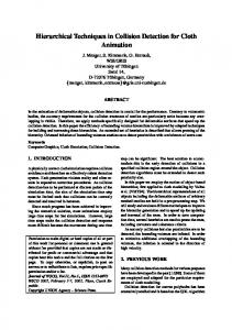
In this section we present a general overview of the V-Clip (Voronoi Clip) and Enhanced GJK (Gilbert, Johnson and Keerthi) algorithms. By describing the algorithms clearly, and highlighting their complete lack of similarity we hope to show the generality of our approach to collision detection algorithm analysis. V-Clip All feature-based schemes are broadly based on the Lin-Canny [Lin93a] closest features algorithm. The fastest available scheme is V-Clip [Mirti98a] – which has claimed an almost constant running time. It is interesting to note that, to our knowledge V-Clip is the only algorithm that was specifically developed for use in a physical simulation. Feature based algorithms are based on the following ideas. Given two polytopes, P and Q (the convex hulls of finite sets of points in R3), we partition them into features. A feature is categorized as a vertex, an edge (defined by its two endpoints) or a face (defined by its edges and, consequently their endpoints). Given two fixed points, a and b, and a third moving point, p, it is possible to quickly determine if p is closer to a or b by use of Voronoi regions. If a plane is constructed half way between a and b, perpendicular to the line connecting them, then it is a simple matter of deciding if p lies in the same halfspace as a or b. This can be extended to any number of fixed points, and is known as constructing the Voronoi diagram of the point set. The generalized Voronoi diagram extends this to higher dimensional features. Again, it uses bounding planes associated with a particular feature (rather than a point) to determine if an arbitrary point is closer to one feature than to another. Fig. 1 illustrates the Voronoi cells associated with a vertex, an edge and a face. The construction of the Voronoi cells is a preprocessing task. It is clear that if a point lies inside the cell associated with a feature, then the point is closer to that feature than to any other. Similarly, if two features lie inside each other’s voronoi regions then they are the closest features between the polytopes. Testing for the inclusion of a vertex in a region is a trivial; the vertex is checked for sidedness against the voronoi planes. If is outside the voronoi region the vertex it is said to violate the voronoi plane. Distinguishing between inclusion and exclusion of an edge or face relies on a clipping algorithm.

Voronoi Regions: (a) Face, (b) Edge, (c) Vertex Figure 1 When a feature lies outside a voronoi region, the region is stepped to a neighbour and the check is repeated. The new region is chosen based upon the results of the exclusion test, it will be the neighbour bordering the most violated voronoi plane. Stepping continues in this fashion until the closest features are found. Enhanced GJK This is an iterative method for computing the distance between polytopes. An important difference between the GJK algorithm and the VClip algorithm is that Enhanced GJK has been generalized to deal with all convex objects [Gilbe90a], including implicit surfaces and the VRML (Virtual Reality Mark-up Language) primitives. Hp(s) = max { p• s | p∈P }, s∈Rn Z = Q + P = { q + p | q∈Q, p∈P } M = Q - P = { q - p | q∈Q, p∈P }

(3) (4) (5)

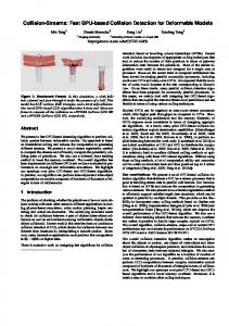
The supporting function, H(p), of a polytope P in direction s is defined in Eq. 3. Since there may be more than one supporting point, we define the contact function as one solution to the above equation. A graphical illustration of a contact function is given in Fig. 2.

When polytopes Q and P collide we can see that they have a common point, q - p = 0 for some p∈P and q∈Q. Thus the Minkowski difference, M, is defined as in Eq. 5 (this is based on the Minkowski sum, Eq. 4, also shown in Fig. 3). When Q and P collide we are sure that 0∈M. The problem of collision detection is now reduced to determining if the origin is contained in M, and the closest pair of points between Q and P is the point on M closest to the origin. It is important to note that the ideas of a supporting function and a contact function are still valid in the context of a Minkowski difference. Subdistance Algorithm (Johnson’s Algorithm) Given a polytope, P = {V1,...,Vm}, P∈Rn,1 < m ≤ ( n + 1), Johnson’s algorithm computes the point, V(p), on P that is closest to the origin. The algorithm is specifically designed to be efficient when the point set is small (at most 4 points in 3-space). The result of the algorithm is expressed in Eq. 7 and Eq. 8 where V(p) is the point closest to the origin and IS is the set of vertices describing the convex hull containing that point. This convex hull will be a simplex (which corresponds to a vertex, and edge or a face) and must be affinely independent or else the algorithm fails. V(p)=∑λiVi (λi∈R) λI > 0, ∑λi = 1, i∈ Is ⊂ {1,..,m}

(7) (8)

The algorithm operates by considering every possible IS. The closest point between the origin and this subset is calculated, and if a termination condition is met then the solution is found. If the termination condition is not met then we proceed to the next possible IS. Two points are worth noting: 1. Computation is not wasted when a possible solution is rejected as the figures computed will be used in a subsequent IS that contain the rejected IS. 2. When testing the subsets we proceed in order of ascending cardinality, thus enabling early acceptance.

s

P

p

Contact function with one supporting vertex Figure 2

Minkowski Sum Figure 3

Gilbert’s Algorithm The purpose of this algorithm is to find the simplex subset of each polytope that contains the point closest to the other polytope. If the algorithm is initialized with two arbitrary simplices, one from each polytope, then a call to Johnson’s algorithm will give us the closest points between these simplices, and possibly a lower dimensional simplex on which each point was found. Taking the direction of the point from the origin in Minkowski space, we can search for new points on the polytopes that may be supporting vertices in these directions. If the new supporting vertices are already known then the algorithm terminates, otherwise we call Johnson’s algorithm again, and repeat the process. Upon termination of the algorithm we have two simplices (each representing a feature on a polytope) and a point on each polytope that is the closest point to the other polytope. There are several implementations of Enhanced GJK algorithm available [Camer97a] [Chung96a] [Berge99a]. The former implementation is described as "the fastest descendent of GJK" [Mirti98a]. The primary performance gain is achieved through intelligent, rather than brute force, selection of supporting vertices (smart evaluation of the contact function). In a simple implementation, finding a supporting vertex in direction s would take O(n) time - the supporting function would be evaluated for each of the n vertices of the polytope. By taking into account the convex nature of the polyhedron (the fact that it is a polytope), a hill climbing approach can be employed. Starting with an arbitrary vertex, V, its support function is evaluated, followed by that of its neighbours. If none of the neighbours has a greater support function than V, the algorithm terminates with V as the supporting vertex, otherwise it steps to the greatest neighbour and repeats the process. Implementing a hill climbing scheme reduces the complexity to O(log n). Also, owing to the temporal and spatial coherence of time steps in a simulation, it is often the case that the support vertices of the two polytopes will not have changed, or will have changed to near neighbours of the previous solution. Thus the supporting vertices are cached between time frames.

RESULTS AND ANALYSIS

Test timings were averaged over 30,000 iterations at each sample point in order to smooth experimental errors. From the results it is clear that the V-Clip algorithm runs slightly faster than Enhanced GJK, but the time complexities are comparable. Performance In the static tests V-Clip took an average of 3.98×10-5s for each detection compared to 3.43×10-5s with Enhanced GJK. This results seems to contradict the dynamic test results, Fig. 4, where V-Clip is clearly faster. This anomaly can be explained by the caching system employed by each algorithm, and thus suggests that the caching policy used with V-Clip is significantly more beneficial that that of Enhanced GJK.

With a large foot-print, and poor locality of reference characteristics the resulted in large amounts of memory swapping – or thrashing.

300

Number of tests

4.

0 Number of primitives

0

600

Number of primitives vs. Number of tests Figure 5.

7.E-05

GJK

V-Clip

Time (s)

Time (s)

3.E-05

0.E+00 GJK

0.00

V-Clip

0.E+00 0.1

Linear Velocity (m/s)

Angular Velocity (rad/s)

12.57

Angular Velocity vs. Time (8 vertices) Figure 6.

1.5

Linear Velocity vs. Time Figure 4. 1.E-04 GJK

V-Clip

Time (s)

In the dynamic tests V-Clip is shown to perform slightly faster, but the algorithms are of comparable time complexity. Thus, the performance metric shows that V-Clip is a better choice where lowest detection times are the most important factor. Scalability Scalability in the number of primitives is shown to be linear (Fig. 5), a direct consequence of employing a sweep and prune broad phase to reduce the complexity from O(n2) (pairwise detection) to O(n). When considering primitive complexity both algorithms scaled as expected, with V-Clip consistently out-performing Enhanced GJK, these results are shown in Fig. 6, Fig. 7, and Fig. 8. The most surprising result is shown in Fig. 8 where a model of 386 vertices was used. Enhanced GJK performs as it did with both 8 and 38 vertices, whereas V-Clip behaves erratically. Upon further investigation we discovered that the V-Clip voronoi regions were consuming vast amounts of memory for such a complex primitive, and in our test environment of hundreds of such primitives we were consuming all available memory.

0.E+00 1


7


The significant memory overhead of the V-Clip data structures is highlighted as a notable short coming of the algorithm. Using double precision floating point number, each additional edge requires 168 bytes of feature space information (using single precision halves the overhead). These data structures also have the disadvantage of having to be pre-computed, adding not insignificant complexity to a system with deformable or fracturing models.

1.2E-03 V-Clip

Time (s)

GJK

0.0E+00 1


7


Robustness In our complete suite of tests we did not encounter one single case of algorithm failure. This result may suggest that a robustness metric is superfluous in a comparative study, even though it was invaluable in proving our implementations. In spite of this result, we still believe this to be a vital measure of an algorithm’s stability in the face of degenerate situations – it is a valid result to report zero failures rather than take no measurement at all. Ease of implementation Both of the algorithms considered use a tolerance parameter to decide the lowest allowable separating distance before a collision is reported. Even keeping these parameters ~10-5 presented us with no difficulties. Numerical problems do arise once the tolerance factor falls closer to the numerical precision limits on the chosen processor. The V-Clip algorithm requires substantial pre-processing to build the voronoi region associated with each feature. Aside from the time taken (which is frequently discounted in comparisons), the prebuilt regions require substantial amounts of memory, 168 bytes for every edge in the model. A further disadvantage of pre-processing is the restriction imposed on dynamically deforming the models – every deformation will require the regions to be modified or re-built. Enhanced GJK suffers none of these drawbacks and proves to be a better choice for deforming primitives. 5.

CONCLUSIONS AND FUTURE WORK

The metrics employed show some clear differences between Enhanced GJK and V-Clip, but in most areas performance is very similar. This is unsurprising, as Enhanced GJK is a numerical analog of the feature stepping algorithm. The considerable differences in performance as the primitive complexity increases is caused by the data structures employed by V-Clip. Each additional edge requires

168 bytes of storage, thus with large models the feature stepping algorithm is constantly trashing the fast access on-board cache of most modern processors. We believe that these results demonstrate the usefulness of the metrics we have developed; they clearly show the differences between two algorithms with very similar performance characteristics, but very different low-level (implementation) properties. Without our new metrics it would not have been possible to explicitly state these differences. Currently our research is focussing on the application of our metrics to methods that use bounding volume hierarchies, such as OBB Trees [Kloso97a] and k-DOPs [Gotts22a]. Through testing these algorithms we would like to show the universality of our approach to the problem of evaluating collision detection schemes. 6.

ACKNOWLEDGEMENTS

The authors would like to thank Brian Mirtich and Stephen Cameron for their help in understanding the workings of V-Clip and Enhanced GJK respectively. We would also like to thank Telekinesys Research Ltd., for use of the OmniateTM dynamics environment. REFERENCES [Aggar88a] Aggarwal, A., Chazelle, B., Guibas, L., Ó’Dúnlaing, C., Yap, C., Parallel Computational Geometry, Algorithmica, 3: pp. 293-327, 1988. [Baraf92a] Baraff, David, Lecture Notes for the SIGGRAPH '92 Course "An Introduction to Physically Based Modeling", July 27, 1992, ACM Siggraph '92. [Berge99a] Van Den Bergen, Gino, A Fast and Robust GJK Implementation for Collision Detection of Convex Objects, submitted to Journal of Graphics Tools and currently under review. [Camer97a] Cameron, Stephen, Enhancing GJK: Computing Minimum and Penetration Distances between Convex Polyhedra, International Conference on Robotics and Automation, Albuquerque, 22-24 April 1997. ©IEEE 1997. [Chung96a] Chung Tat Leung, Kelvin, An Efficient Collision Detection Algorithm for Polytopes in Virtual Environments, M. Phil Thesis, University of Hong Kong, 1996. [Chung96b] Chung, Kelvin, Wenping, Wang, Quick Elimination of Non-Interference Polytopes in Virtual Environments, ACM Symposium on Virtual Reality Software and Technology, 1996

[Cohen95a] Cohen, Jonathan D., Lin, Ming C., Manocha, Dinesh, Ponamgi, Madhav K., ICOLLIDE: An Interactive and Exact Collision Detection System for Large-Scale Environments, Proceedings of ACM Int. 3D Graphics Conference , pp. 189-196, 1995. [Gilbe88a] Gilbert, E. G., Johnson, D. W., Keerthi, S. S., A fast procedure for computing the distance between objects in three-dimensional space. IEEE Journal on Robotics and Automation, vol RA-4:pp. 193-203, 1988. [Gilbe90a] Gilbert, E. G., Foo, C. P., Computing the distance between general convex objects in three-dimensional space, IEEE Transactions on Robotics and Automation, 6(1) pp. 53-61, 1990. [Gotts96a] Gottschalk, S., Lin, M. C., Manocha, D., OBBTree: A Hierarchical Structure for Rapid Interference Detection, Proceedings of ACM Siggraph ‘96, 1996. [Gotts96b] Gottschalk, S., Separating Axis Theorem, Technical Report TR96-024, Department of Computer Science, UNC Chapel Hill, 1996. [Held95a] Held, Martin, Klosowski, James T., Mitchell, Joseph S. B., Evaluation of Collision Detection Methods for Virtual Reality Fly-Throughs, Proc. 7th Canad. Conf. Computat. Geometry, Québec, Canada, Aug 10-13, 1995. [Held95b] Held, M., Klosowski, J. T., Mitchell, J. S. B., Speed Comparison of Generalized Bounding Box Hierarchies. Technical Report, Department of Applied Math, SUNY Stony Brook, 1995. [Hubba95a] Hubbard, Philip M., Real-Time Collision Detection and Time-Critical Computing, Workshop on Simulation and Interaction in Virtual Environments, July 1995. [Kloso97a] Klosowski, James T., Held, Martin, Mitchell, Joseph S. B., Sowizral, Henry, Zikan, Karel, Efficient Collision Detection Using Bounding Volume Hierarchies of kdops, IEEE Transactions on Visualisation and Computer Graphics, 1997. [Len92a] Len, W., Fusco, M., Fast n-dimension extent overlap testing, Graphics Gems III, AP Professional, pp. 240-243, 1992. [Lin93a] Lin, Ming C., Efficient Collision Detection for Animation and Robotics. PhD thesis, University of California, Berkeley, 1993. [Lin98a] Lin, Ming C., Gottschalk, Stefan, Collision Detection between Geometric Models: A Survey, Proceedings of IMA Conference on Mathematics of Surfaces, 1998. [Mirti96a] Mirtich, Brian Vincent, Impulse-based Dynamic Simulation of Rigid Body Systems, PhD thesis, University of California, Berkeley, 1996.

[Mirti98a] Mirtich, Brian, V-Clip: Fast and Robust Polyhedral Collision Detection. ACM Transactions on Graphics, 1998. [Rabbi94a] Rabbitz, Rich, Fast Collision Detection of Moving Convex Polyhedra, Graphics Gems IV, pages 83-109, Heckbert, P., editor, Academic Press, Boston MA, 1994. [Welzl91a] Welzl, Emo, Smallest enclosing disks (balls and ellipsoids), Lecture Notes in Computer Science 555, pp. 359-370, 1991. [Wilhe88a] Wilhelms, Moore, Collision Detection using Beck Line Clipping, SIGGRAPH ’88, Conference proceedings, p. 289.