Ideally, this procedure should not change the basic symmetries of the .... Hy(x, t) and the electric field Ez(x, t) of the TM-mode in the 1D cavity of length L are.
ICAP 2002
New numerical methods for solving the time-dependent Maxwell equations H. De Raedt, J.S. Kole, K.F.L. Michielsen, and M.T. Figge Applied Physics - Computational Physics‡, Materials Science Centre University of Groningen, Nijenborgh 4, NL-9747 AG Groningen, The Netherlands Abstract. We review some recent developments in numerical algorithms to solve the time-dependent Maxwell equations for systems with spatially varying permittivity and permeability. We show that the Suzuki product-formula approach can be used to construct a family of unconditionally stable algorithms, the conventional Yee algorithm, and two new variants of the Yee algorithm that do not require the use of the staggered-in-time grid. We also consider a one-step algorithm, based on the Chebyshev polynomial expansion, and compare the computational efficiency of the one-step, the Yee-type and the unconditionally stable algorithms. For applications where the longtime behavior is of main interest, we find that the one-step algorithm may be orders of magnitude more efficient than present multiple time-step, finite-difference time-domain algorithms.
1. Introduction The Maxwell equations describe the evolution of electromagnetic (EM) fields in space and time [1]. They apply to a wide range of different physical situations and play an important role in a large number of engineering applications. In many cases, numerical methods are required to solve Maxwell’s equations [2, 3]. A well-known class of algorithms is based on a method proposed by Yee [4]. This finite-difference timedomain (FDTD) approach owes its popularity mainly due to its flexibility and speed while at the same time it is easy to implement [2, 3]. A limitation of Yee-based FDTD techniques is that their stability is conditional, depending on the mesh size of the spatial discretization and the time step of the time integration [2, 3]. Furthermore, in practice, the amount of computational work required to solve the time-dependent Maxwell equations by present FDTD techniques [2, 3, 5, 6, 7, 8, 9, 10, 11, 12] prohibits applications to a class of important fields such as bioelectromagnetics and VLSI design [2, 13, 14]. The basic reason for this is that the time step in the FDTD calculation has to be relatively small in order to maintain stability and a reasonable degree of accuracy in the time integration. Thus, the search for new algorithms that solve the Maxwell equation focuses on removing the ‡ http://www.compphys.org/
Numerical methods for solving the time-dependent Maxwell equations
2
conditional stability of FDTD methods and on improving the accuracy/efficiency of the algorithms. 2. Time integration algorithms We consider EM fields in linear, isotropic, nondispersive and lossless materials. The time evolution of EM fields in these systems is governed by the time-dependent Maxwell equations [1]. Some important physical symmetries of the Maxwell equations √ can be made explicit by introducing the fields X(t) ≡ µH(t) and Y(t) ≡ √ T εE(t). Here, H(t) = (Hx (r, t), Hy (r, t), Hz (r, t)) denotes the magnetic and E(t) = (Ex (r, t), Ey (r, t), Ez (r, t))T the electric field vector, while µ = µ(r) and ε = ε(r) denote, respectively, the permeability and the permittivity. Writing Z(t) = (X(t), Y(t))T , Maxwell’s curl equations [2] read
∂ Z(t) = ∂t
0 1 √ ∇× ε
√1 µ
− √1µ ∇ × 0
√1 ε
Z(t) ≡ HZ(t).
(1)
It is easy to show that H is skew symmetric, i.e. HT = −H, with respect to the inner � product �Z(t)|Z� (t) ≡ V ZT (t) · Z� (t) dr, where V denotes the system’s volume. In √ √ addition to Eq.(1), the EM fields also satisfy ∇ · ( µX(t)) = 0 and ∇ · ( εY(t)) = 0 [1]. Throughout this paper we use dimensionless quantities: We measure distances in units of λ and expresss time and frequency in units of λ/c and c/λ, respectively. A numerical algorithm that solves the time-dependent Maxwell equations necessarily involves some discretization procedure of the spatial derivatives in Eq. (1). Ideally, this procedure should not change the basic symmetries of the Maxwell equations. We will not discuss the (important) technicalities of the spatial discretization (we refer the reader to Refs. [2, 3]) as this is not essential to the discussion that follows. On a spatial grid Maxwell’s curl equations (1) can be written in the compact form [11] ∂ Ψ(t) = HΨ(t). (2) ∂t The vector Ψ(t) is a representation of Z(t) on the grid. The matrix H is the discrete analogue of the operator H. The formal solution of Eq. (2) is given by Ψ(t) = etH Ψ(0) = U (t)Ψ(0),
(3)
where U (t) = etH denotes the time-evolution matrix. If the discretization procedure preserves the underlying symmetries of the time-dependent Maxwell equations then the matrix H is real and skew symmetric, implying that U (t) is orthogonal [15]. Physically, the orthogonality of U (t) implies conservation of energy. There are two, closely related, strategies to construct an algorithm for performing the time integration of the time-dependent Maxwell equations defined on the grid [16]. The traditional approach is to discretize (with increasing level of sophistication) the derivative with respect to time [16]. The other is to approximate the formally exact solution, i.e. the matrix exponential U (t) = etH by some time evolution matrix
Numerical methods for solving the time-dependent Maxwell equations
3
U� (t) [16, 17]. We adopt the latter approach in this paper as it facilitates the construction of algorithms with specific features, such as unconditional stability [17]. If the approximation U� (t) is itself an orthogonal transformation, then U� (t) = 1 where X denotes 2-the norm of a vector or matrix X [15]. This implies that U� (t)Ψ(0) = Ψ(0) , for an arbitrary initial condition Ψ(0) and for all times t and hence the time integration algorithm defined by U� (t) is unconditionally stable by construction [16, 17]. We now consider two options to construct the approximate time evolution matrix � U (t). The first approach yields the conventional Yee algorithm, a higher-order generalization thereof, and the unconditional schemes proposed in Ref.[11]. Second, the Chebyshev polynomial approximation to the matrix exponential [18, 19, 20, 21, 22, 23]. is used to construct a one-step algorithm [24, 25]. 2.1. Suzuki product-formula approach A systematic approach to construct approximations to matrix exponentials is to make use of the Lie-Trotter-Suzuki formula [26, 27] etH = et(H1 +...+Hp ) = lim m→∞
� p �
etHi /m
m
,
(4)
i=1
and generalizations thereof [28, 29]. Expression Eq. (4) suggests that U1 (τ ) = eτ H1 . . . eτ Hp ,
(5)
might be a good approximation to U (τ ) if τ is sufficiently small. Applied to the case of interest here, if all the Hi are real and skew-symmetric U1 (τ ) is orthogonal by construction and a numerical scheme based on Eq. (5) will be unconditionally stable. For small τ , the error U (t = mτ ) − [U1 (τ )]m vanishes like τ [29] and therefore we call U1 (τ ) a first-order approximation to U (τ ). The product-formula approach provides simple, systematic procedures to improve the accuracy of the approximation to U (τ ) without changing its fundamental symmetries. For example the matrix U2 (τ ) = U1 (−τ /2)T U1 (τ /2) = eτ Hp /2 . . . eτ H1 /2 eτ H1 /2 . . . eτ Hp /2 ,
(6)
is a second-order approximation to U (τ ) [28, 29]. If U1 (τ ) is orthogonal, so is U2 (τ ). Suzuki’s fractal decomposition approach [29] gives a general method to construct higherorder approximations based on U2 (τ ) (or U1 (τ )). A particularly useful fourth-order approximation is given by [29] U4 (τ ) = U2 (aτ )U2 (aτ )U2 ((1 − 4a)τ )U2 (aτ )U2 (aτ ),
(7)
where a = 1/(4 − 41/3 ). In practice an efficient implementation of the first-order scheme is all that is needed to construct the higher-order algorithms Eqs.(6) and (7). The crucial step of this approach is to choose the Hi ’s such that the matrix exponentials exp(τ H1 ), ..., exp(τ Hp ) can be calculated efficiently. This will turn the formal expressions for U2 (τ ) and U4 (τ ) into efficient algorithms to solve the time-dependent Maxwell equations.
Numerical methods for solving the time-dependent Maxwell equations
4
2.2. One-step algorithm The basic idea of this approach is to make use of extremely accurate polynomial approximations to the matrix exponential. We begin by “normalizing” the matrix H. The eigenvalues of the skew-symmetric matrix H are pure imaginary numbers.
In practice H is sparse so it is easy to compute H 1 ≡ maxj i |Hi,j |. Then, by construction, the eigenvalues of B ≡ −iH/ H 1 all lie in the interval [−1, 1] [15]. Expanding the initial value Ψ(0) in the (unknown) eigenvectors bj of B, Eq. (3) reads Ψ(t) = eizB Ψ(0) =
� j
eizbj bj �bj |Ψ(0) ,
(8)
where z = t H 1 and the bj denote the (unknown) eigenvalues of B. There is no need to know the eigenvalues and eigenvectors of B explicitly. We find the Chebyshev polynomial expansion of U (t) by computing the expansion coefficients of each of the functions eizbj that appear in Eq. (8). In particular, as −1 ≤ bj ≤ 1, we can use the
k expansion [30] eizbj = J0 (z) + 2 ∞ k=1 i Jk (z)Tk (bj ) , where Jk (z) is the Bessel function of integer order k, to write Eq. (8) as
Ψ(t) = J0 (z)I + 2
∞ �
Jk (z)Tˆk (B) Ψ(0) .
(9)
k=1
Here Tˆk (B) = ik Tk (B) is a matrix-valued modified Chebyshev polynomial that is defined by Tˆ0 (B)Ψ(0) = Ψ(0), Tˆ1 (B)Ψ(0) = iBΨ(0) and the recursion Tˆk+1 (B)Ψ(0) = 2iB Tˆk (B)Ψ(0) + Tˆk−1 (B)Ψ(0) ,
(10)
for k ≥ 1. As Tˆk (B) ≤ 1 by construction and |Jk (z)| ≤ |z|k /2k k! for z real [30], the resulting error vanishes exponentially fast for sufficiently large K. Thus, we can obtain an accurate approximation by summing contributions in Eq. (9) with k ≤ K only. The number K is fixed by requiring that |Jk (z)| < κ for all k > K. Here, κ is a control parameter that determines the accuracy of the approximation. For fixed κ, K increases linearly with z = t H 1 (there is no requirement on t being small). From numerical analysis it is known that for fixed K, the Chebyshev polynomial is very nearly the same polynomial as the minimax polynomial [31], i.e. the polynomial of degree K that has the smallest maximum deviation from the true function, and is much more accurate than for instance a Taylor expansion of the same degree K. In practice, K ≈ z. In a strict sense, the one-step method does not yield an orthogonal approximation. However, for practical purposes it can be viewed as an extremely stable time-integration algorithm because it yields an approximation to the exact time evolution operator U (t) = etH that is exact to nearly machine precision [24, 25]. This also implies that within the same precision ∇·(µH(t)) = ∇·(µH(t = 0)) and ∇·(εE(t)) = ∇·(εE(t = 0)) holds for all times, implying that the numerical scheme will not produce artificial charges during the time integration [2, 3].
Numerical methods for solving the time-dependent Maxwell equations
5
3. Implementation The basic steps in the construction of the product-formula and one-step algorithms are best illustrated by considering the simplest case, i.e. the Maxwell equations of a 1D homogeneous problem. From a conceptual point of view nothing is lost by doing this: the extension to 2D and 3D nonhomogeneous problems is straigthforward, albeit technically non-trivial [11, 12, 24, 25]. We consider a system, infinitely large in the y and z direction, for which ε = 1 and µ = 1. Under these conditions, the Maxwell equations reduce to two independent sets of first-order differential equations [1], the transverse electric (TE) mode and the transverse magnetic (TM) mode [1]. As the equations of the TE- and TM-mode differ by a sign we can restrict our considerations to the TM-mode only. The magnetic field Hy (x, t) and the electric field Ez (x, t) of the TM-mode in the 1D cavity of length L are solutions of ∂ ∂ ∂ ∂ (11) Hy (x, t) = Ez (x, t) , Ez (x, t) = Hy (x, t), ∂t ∂x ∂t ∂x subject to the boundary condition Ez (0, t) = Ez (L, t) = 0 [1]. Note that the divergence of both fields is trivially zero. Following Yee [4], to discretize Eq.(11), it is convenient to assign Hy to odd and Ez to even numbered lattice sites. Using the second-order central-difference approximation to the first derivative with respect to x, we obtain ∂ (12) Hy (2i + 1, t) = δ −1 (Ez (2i + 2, t) − Ez (2i, t)), ∂t ∂ (13) Ez (2i, t) = δ −1 (Hy (2i + 1, t) − Hy (2i − 1, t)), ∂t where we have introduced the notation A(i, t) = A(x = iδ/2, t). The integer i labels the grid points and δ denotes the distance between two next-nearest neighbors on the lattice (hence the absence of a factor two in the nominator). We define the n-dimensional vector Ψ(t) by �
Ψ(i, t) =
Hy (i, t), i odd . Ez (i, t), i even
(14)
The vector Ψ(t) contains both the magnetic and the electric field on the lattice points i = 1, . . . , n. The i-th element of Ψ(t) is given by the inner product Ψ(i, t) = eTi · Ψ(t) where ei denotes the i-th unit vector in the n-dimensional vector space. Using this notation (which proves most useful for the case of 2D and 3D for which it is rather cumbersome to write down explicit matrix representations), it is easy to show that Eqs.(12) and (13) can be written in the form (2) where the matrix H is given by
0 δ −1 −δ −1 0 . .. H=
δ −1 ... −δ −1
... 0 −δ −1
n−1 � �� = δ −1 ei eTi+1 − ei+1 eTi .(15) i=1 δ −1
0
Numerical methods for solving the time-dependent Maxwell equations
6
We immediately see that H is sparse and skew-symmetric by construction. 3.1. Yee-type algorithms First we demonstrate that the Yee algorithm fits into the product-formula approach. For the 1D model (15) it is easy to see that one time-step with the Yee algorithm corresponds to the operation T
U1Y ee (τ ) = (I + τ A)(I − τ AT ) = eτ A e−τ A ,
(16)
where A = δ −1
n−1 � � � i=2
�
ei eTi−1 − ei eTi+1 ,
(17)
and we used the arrangements of H and E fields as defined by Eq.(14). We use the
notation � to indicate that the stride of the summation index is two. Note that since A2 = 0 we have eτ A = 1+τ A exactly. Therefore we recover the timestep operator of the Yee algorithm using the first-order product formula approximation to eτ H and decomposing H = A − AT . However, the Yee algorithm is second-order, not first order, accurate in time [2, 3]. This is due to the use of a staggered grid in time [2, 3]. To perform one time step with the Yee algorithm we need to know the values of Ez (t) and Hy (t + τ /2), not Hy (t). Another method has to supply the Hy -field at a time shifted by τ /2. Within the spirit of this approach, we can easily eliminate the staggered-in-time grid at virtually no extra computational cost or progamming effort (if a conventional Yee code is available) by using the second-order product formula T
U2Y ee (τ ) = eτ A/2 e−τ A eτ A/2 = (I + τ A/2)(I − τ AT )(I + τ A/2).
(18)
The effect of the last factor is to propagate the Hy -field by τ /2. The middle factor propagates the Ez -field by τ . The first factor again propagates the Hy field by τ /2. In this scheme all EM fields are to be taken at the same time. The algorithm defined by U2Y ee (τ ) is second-order accurate in time by construction [17]. Note that eτ A/2 is not orthogonal so nothing has been gained in terms of stability. Since [U2Y ee (τ )]m = e−τ A/2 [U1Y ee (τ )]m e+τ A/2 , we see that, compared to the original Yee algorithm, the extra computational work is proportional to (1 + 2/m), hence negligible if the number of time steps m is large. According to the general theory outlined in Sec.2, the expression U4Y ee (τ ) = U2Y ee (aτ )U2Y ee (aτ )U2Y ee ((1 − 4a)τ )U2Y ee (aτ )U2Y ee (aτ ),
(19)
defines a fourth-order accurate Yee-like scheme, the realization of which requires almost no effort once U2Y ee has been implemented. It is easy to see that the above construction of the Yee-like algorithms holds for the much more complicated 2D, and 3D inhomogeneous case as well. Also note that the fourth-order Yee algorithm U4Y ee does not require extra storage to hold field values at intermediate times.
Numerical methods for solving the time-dependent Maxwell equations
7
3.2. Unconditionally stable algorithms Guided by previous work on Schr¨odinger and diffusion problems [17], we split H into two parts H1 = δ H2 = δ
−1
n−1 � � �
i=1 n−2 �� −1 i=1
�
�
ei eTi+1 − ei+1 eTi ,
(20) �
ei+1 eTi+2 − ei+2 eTi+1 .
(21)
such that H = H1 + H2 . In other words we divide the lattice into odd and even numbered cells. According to the general theory given above, the first-order algorithm is given by U�1 (τ ). Clearly both H1 and H2 are skew-symmetric block-diagonal matrices, containing one 1 × 1 matrix and (n − 1)/2 real, 2 × 2 skew-symmetric matrices. As the matrix exponential of a block-diagonal matrix is equal to the block-diagonal matrix of the matrix exponentials of the individual blocks, the numerical calculation of eτ H1 (or eτ H2 ) reduces to the calculation of (n − 1)/2 matrix exponentials of 2 × 2 matrices. Each of these matrix exponentials only operates on a pair of elements of Ψ(t) and leaves other elements intact. The indices of each of these pairs are given by the subscripts of e and eT . Using the U�1 (τ ) algorithm it is easy to construct the unconditionally stable, higher-order algorithms U�2 (τ ) and U�4 (τ ), see Eq.(6) and Eq.(7). 3.3. One-step algorithm The one-step algorithm is based on the recursion Eq.(10). Thus, the explicit form Eq.(15) is all we need to implement the matrix-vector operation (i.e. Ψ� ← HΨ) that enters Eq.(10). The coefficients Jk (z) (and similar ones if a current source is present) should be calculated to high precision. Using the recursion relation of the Bessel functions, all K coefficients can be obtained with O(K) arithmetic operations [31], a neglible fraction of the total computational cost for solving the Maxwell equations. Performing one time step amounts to repeatedly using recursion (10) to obtain ˆ Tk (B)Ψ(0) for k = 2, . . . , K, multiply the elements of this vector by the appropiate coefficients and add all contributions. This procedure requires storage for two vectors of the same length as Ψ(0) and some code to multiply such a vector by the sparse matrix H. The result of performing one time step yields the solution at time t, hence the name one-step algorithm. In contrast to what Eq.(10) might suggest, the algorithm does not require the use of complex arithmetic. 4. Numerical experiments Except for the conventional Yee algorithm, all algorithms discussed in this paper operate on the vector of fields defined at the same time t. We use the one-step algorithm (with a time step τ /2) to compute Ez (τ /2) and Hy (τ /2). Then we use Ez (0) and Hy (τ /2) as the initial values for the Yee algorithm. In order to permit comparison of the final
Numerical methods for solving the time-dependent Maxwell equations
8
2
log (error)
0 -2 -4 Yee U2(Yee) U2 U4(Yee) U4
-6 -8 -10 -3.5
-3
-2.5
-2
-1.5
-1
-0.5
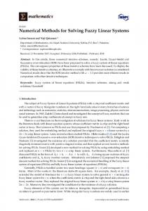
log (time step) ˜ ˆ ˆ Figure 1. The error Ψ(t) − Ψ(t) / Ψ(t) at time t = 100 as a function of the time step τ for five different FDTD algorithms, plotted on a double logarithmic scale. The initial values of the EM fields are random, distributed uniformly over the interval [-1,1], on a grid of n = 5001 sites with δ = 0.1 (corresponding to a physical length of 250.05). ˆ Ψ(t) is the vector obtained by the one-step algorithm κ = 10−9 , using K = 2080 matrix-vector operations Ψ� ← M Ψ. The results of the Yee and U2Y ee algorithm lie on top of each other. Lines are guides to the eye.
result of the conventional Yee algorithm with those of the other methods, we use the one-step algorithm once more to shift the time of the Hy field by −τ /2. This procedure to prepare the initial and to analyse the final state of the Yee algorithm does in fact make the results of the Yee algorithm look a little more accurate than they would be if the exact data of the τ /2-shifted fields were not available. ˜ ˜ ˆ ˆ We define the error of the solution Ψ(t) for the wave form by Ψ(t)− Ψ(t) / Ψ(t) ˆ where Ψ(t) is the vector of EM fields obtained by the one-step algorithm. Thereby we have already assumed that the one-step algorithm yields the exact (within numerical precision) results but this has to be demonstrated of course. A comparison of the results of an unconditionally stable algorithm, e.g. U�4 with those of the one-step algorithm is sufficient to show that within rounding errors the latter yields the exact answer. ˆ ˜ ˜ ˆ Using the triangle inequality Ψ(t) − Ψ(t) ≤ Ψ(t) − Ψ(t) + Ψ(t) − Ψ(t) and 4 ˜ the rigorous bound Ψ(t) − Ψ(t) ≤ c4 τ t Ψ(0) [17], we can be confident that the one-step algorithm yields the numerically exact answer if i) this rigorous bound is not ˜ ˆ violated and ii) if Ψ(t) − Ψ(t) vanishes like τ 4 . From the data in Fig.1 we conclude that the error of algorithm U�4 vanishes like τ 4 , demonstrating that the one-step algorithm yields the numerically exact result. The high precision of the one-step algorithm also allows us to use it for genuine time stepping with
Numerical methods for solving the time-dependent Maxwell equations
9
arbitrarily large time steps, this in spite of the fact that strictly speaking, the one-step algorithm is not unconditionally stable. If the initial EM field distribution is random then, for sufficiently small τ , algorithm � U2 is more accurate than the two second-order accurate Yee algorithms, as is clear from Fig.1 [32]. However, this conclusion is biased by the choice of the model problem and does not generalize. For the largest τ -values used in Fig.1, the Yee and U2Y ee algorithm are operating at the point of instability, signaled by the fact that the norm of Ψ(t) grows rapidly, resulting in errors that are very large. If the initial state is a Gaussian wave packet that is fairly broad, the Yee-type algorithms are much more accurate than the unconditionally stable algorithms employed in this paper (results not shown). The data of Fig.1 clearly show that for all algorithms, the expected behavior of the error as a function of τ is observed only if τ is small enough. The answer to the question which of the algorithms is the most efficient one crucially depends on the accuracy that one finds acceptable. The Yee algorithm is no competition for U�4 if one requires an error of less than 1% but then U�4 is not nearly as efficient (by a factor of about 6) as the one-step algorithm. Increasing the dimensionality of the problem favors the one-step algorithm [24, 25]. These conclusions seem to be quite general and are in concert with numerical experiments on 1D, 2D and 3D systems [25]. A simple theoretical analysis of the τ dependence of the error shows that the one-step algorithm is more efficient than any other FDTD method if we are interested in the EM fields at a particular (large) time only [24, 25]. This may open possibilities to solve problems in computational electrodynamics that are currently intractable. The Yee-like algorithms do not conserve the energy of the EM fields and therefore they are less suited for the calculation of the eigenvalue distributions (density of states), a problem for which the U�4 algorithm may be the most efficient of all the algorithms covered in the paper. The main limitation of the one-step algorithm lies in its mathematical justification. The Chebyshev approach requires that H is diagonalizable and that its eigenvalues are real or pure imaginary. The effect of relaxing these conditions on the applicability of the Chebyshev approach is left for future research. In this paper we have focused entirely on the accuracy of the time integration algorithms, using the most simple discretization of the spatial derivatives. For practical purposes, this is often not sufficient. In practice it is straightforward, though technically non-trivial, to treat more sophisticated discretization schemes [2, 12] by the methodology reviewed is this paper. Acknowledgments H.D.R. and K.M. are grateful to T. Iitaka for drawing our attention to the potential of the Chebyshev method and for illuminating discussions. This work is partially supported by the Dutch ‘Stichting Nationale Computer Faciliteiten’ (NCF), and the EC IST project CANVAD.
Numerical methods for solving the time-dependent Maxwell equations
10
References [1] M. Born and E. Wolf, Principles of Optics, (Pergamon, Oxford, 1964). [2] A. Taflove and S.C. Hagness, Computational Electrodynamics - The Finite-Difference TimeDomain Method, (Artech House, Boston, 2000). [3] K.S. Kunz and R.J. Luebbers, Finite-Difference Time-Domain Method for Electromagnetics, (CRC Press, 1993). [4] K.S. Yee, IEEE Transactions on Antennas and Propagation 14, 302 (1966). [5] See http://www.fdtd.org [6] F. Zheng, Z. Chen, and J. Zhang, IEEE Trans. Microwave Theory and Techniques 48, 1550 (2000). [7] T. Namiki, IEEE Trans. Microwave Theory and Techniques 48, 1743 (2001). [8] F. Zheng and Z. Chen, IEEE Trans. Microwave Theory and Techniques 49, 1006 (2001). [9] S.G. Garcia, T.W. Lee, S.C. Hagness, IEEE Trans. and Wireless Prop. Lett. 1, 31 (2002). [10] W. Harshawardhan, Q. Su, and R. Grobe, Phys. Rev. E 62, 8705 (2000). [11] J.S. Kole, M.T. Figge and H. De Raedt, Phys. Rev. E 64, 066705 (2001). [12] J.S. Kole, M.T. Figge and H. De Raedt, Phys. Rev. E 65, 066705 (2002). [13] O.P. Gandi, Advances in Computational Electrodynamics - The Finite-Difference Time-Domain Method, A. Taflove, Ed., (Artech House, Boston, 1998). [14] B. Houshmand, T. Itoh, and M. Piket-May, Advances in Computational Electrodynamics - The Finite-Difference Time-Domain Method, A. Taflove, Ed., (Artech House, Boston, 1998). [15] J.H. Wilkinson, The Algebraic Eigenvalue Problem, (Clarendon Press, Oxford, 1965). [16] G.D. Smith, Numerical solution of partial differential equations, (Clarendon Press, Oxford, 1985). [17] H. De Raedt, Comp. Phys. Rep. 7, 1 (1987). [18] H. Tal-Ezer, SIAM J. Numer. Anal. 23, 11 (1986). [19] H. Tal-Ezer and R. Kosloff, J. Chem. Phys. 81, 3967 (1984). [20] C. Leforestier, R.H. Bisseling, C. Cerjan, M.D. Feit, R. Friesner, A. Guldberg, A. Hammerich, G. Jolicard, W. Karrlein, H.-D. Meyer, N. Lipkin, O. Roncero, and R. Kosloff, J. Comp. Phys. 94, 59 (1991). [21] T. Iitaka, S. Nomura, H. Hirayama, X. Zhao, Y. Aoyagi, and T. Sugano, Phys. Rev. E 56, 1222 (1997). [22] R.N. Silver and H. R¨ oder, Phys. Rev. E 56, 4822 (1997). [23] Y.L. Loh, S.N. Taraskin, and S.R. Elliot, Phys. Rev. Lett. 84, 2290 (2000); ibid. Phys.Rev.Lett. 84, 5028 (2000). [24] H. De Raedt, K. Michielsen, J.S. Kole, and M.T. Figge, in Computer Simulation Studies in Condensed-Matter Physics XV, eds. D.P. Landau et al., Springer Proceedings in Physics, (Springer, Berlin, in press). [25] H. De Raedt, K. Michielsen, J.S. Kole, and M.T. Figge, submitted to IEEE Antennas and Propagation, LANL prepint: physics/0208060 [26] M. Suzuki, S. Miyashita, and A. Kuroda, Prog. Theor. Phys. 58, 1377 (1977). [27] H.F. Trotter, Proc. Am. Math. Soc. 10, 545 (1959). [28] H. De Raedt and B. De Raedt, Phys. Rev. A 28, 3575 (1983). [29] M. Suzuki, J. Math. Phys. 26, 601 (1985); ibid 32 400 (1991). [30] M. Abramowitz and I. Stegun, Handbook of Mathematical Functions, (Dover, New York, 1964). [31] W.H. Press, B.P. Flannery, S.A. Teukolsky, and W.T. Vetterling, Numerical Recipes, (Cambridge, New York, 1986). �4 yield more accurate �2 and U [32] This also explains why the unconditionally stable algorithms U eigenvalue distributions than the Yee algorithm [11].