Pyx. JTyx j j j j θ θ . However, errors-in-variables complicate matters. The influence of errors-in-variables is difficult to assess in general, because it depends on ...
New Tools for Dealing with Errors-in-Variables in DEA Laurens Cherchye Catholic University of Leuven Center for Economic Studies Naamsestraat 69 3000 Leuven, BELGIUM
Timo Kuosmanen Helsinki School of Economics and Business Administration Department of Economics and Management Science P.O. Box 1210, FIN-00101 Helsinki, FINLAND
Thierry Post Erasmus University Rotterdam Department of Finance Burg. Oudlaan 50 3062 PA Rotterdam, THE NETHERLANDS
All rights reserved. This study may not be reproduced in whole or in part without the authors' explicit permission
1
Abstract We develop a series of novel conceptual tools to systematically account for errors-invariables in Data Envelopment Analysis (DEA). These tools allow for statistical inference while requiring minimal statistical distribution assumptions, and therefore constitute a valuable addition to the tools currently available for dealing with errors-in-variables. An empirical application for large European Union financial institutions illustrates the proposed approach. Keywords: Data Envelopment Analysis (DEA), errors-in-variables, efficiency depth, robust reference sets, financial institutions
1. Introduction Data Envelopment Analysis (DEA), originating from Farrell's (1957) work and popularized by Charnes et al. (1978), is a collection of non-parametric methods for evaluating the productive efficiency of Decision Making Units (DMUs). DEA does not require an explicit specification of a functional relationship between inputs and outputs or a statistical distribution for the inefficiencies. These features are the key advantage of DEA over alternative parametric approaches. However, the original DEA methodology requires the production process is completely characterized by the observed input-output variables, which are free of errors. This is generally recognized as the most serious limitation of DEA. In practice, the data sets are almost always incomplete and contaminated by errors. In addition to obvious typographical or measurement errors, there are at least three other important potential sources of errors. Firstly, the use of instrumental variables when data is not available for some relevant inputs or outputs entails the possibility of errors. For example, much empirical research uses accounting data that can give a flawed representation of the underlying economic values, e.g. because of debatable valuation and depreciation schemes. Secondly, aggregation over production establishments, input-output variables and time periods, which is a frequent practice in DEA applications, introduces another potential source of errors. Thirdly, the variables included in the model may not fully account for all omitted input-output variables. Note that the influence of omitted variables could be accounted for by appropriate compensation on the variables included in the model. Ignorance of this compensation when it would be necessary may be viewed as an error in the included production variables.
Unfortunately, DEA results are highly sensitive to errors-in-variables, because DEA relies on comparison with extreme observations (see also Sexton et al., 1986). A potential solution to errors-in-variables is to analyse the sensitivity of DEA results with respect to variations in the data (e.g. Charnes et al. (1985), Charnes and Neralic (1990), Charnes et al. (1992) and Zhu (1996)). However, the correct interpretation of the outcomes is not immediately clear in general. For example, sensitivity to a particular data variation is meaningless if that specific variation is highly unlikely. Stochastic DEA models that explicitly account for the statistical distribution of the errors provide another potential solution. In the DEA literature, a number of such 2
models have been proposed (e.g. Gong and Sun (1995), Land et al. (1994), Olesen and Petersen (1995), Post (1997), Cooper et al. (1998), Gstach (1998), and Li (1998)). However, in contrast to the nonparametric nature of the original DEA models, the stochastic models typically require the specification of a particular statistical distribution for the errors. Unfortunately, in many research environments, the specification of the error distribution can not be justified using prior theory or available economic data. In addition, the robustness of stochastic DEA models with respect to erroneous distribution assumptions remains as an open question.
In this paper, we develop a series of novel tools to systematically account for errors-invariables in DEA. We introduce novel concepts including efficiency depth and robust reference sets. These conceptual tools allow for statistical inference while requiring minimal statistical distribution assumptions, and therefore constitute a valuable addition to the tools currently available for dealing with errors-invariables. The rest of the paper is organised as follows. Section 2 discusses the essentials of the original DEA model and the role of errors-in-variables. Section 3 introduces a nonparametric test statistic (efficiency depth) for testing for efficiency in case of errors-in-variables. Section 4 introduces robust reference sets and robust efficiency measures. Section 5 provides Mixed Integer Linear Programming models for computing the test statistic and the robust efficiency measures from empirical data. Section 6 illustrates our approach using an empirical application for large European Union financial institutions. Finally, Section 7 presents our conclusions.
2. The original model DEA is used for evaluating efficiency of the DMUs relative to the "best-practice" production possibilities' frontier. Theoretically, the production possibilities can be represented by the production set: (1)
{
}
P = ( x, y ) ∈ ℜ m+ + s input x can produce output y ,
where x ∈ ℜ m+ and y ∈ ℜ s+ denote input and output vectors respectively. Unfortunately, the production set is typically unknown and has to be approximated using empirical production data of a sample of comparable DMUs. In this study, J represents an index set, and X ( J ) = ( x1 ...x card ( J ) ) T , with x j = ( x1 j ⋅ ⋅ ⋅ xmj ) , and Y ( J ) = ( y1 ... y card ( J ) )T , with y j = ( y1 j ⋅ ⋅ ⋅ y sj ) , represent the input-output vectors for the DMUs in the sample. The original DEA methodology assumes that the production vectors are feasible, i.e.
3
( x j , y j ) ∈ P ∀j ∈ J . In addition, the original methodology assumes the observed values for the input-output variables are free of errors. In this study, we adhere to the assumption that the production vectors are feasible. However, we explicitly assume that the input-output variables may contain errors. Specifically, we assume the true values are not observed and that only inaccurate estimates are available, that randomly deviate from the true values1. In the analysis below, we will let (2)
yˆ rj = y rj + wrj′
(3)
xˆ ij = xij + wij
r = 1,..., s; j = 1,..., card ( J ) , i = 1,..., m; j = 1,..., card ( J )
represent the estimated values, where wrj′ (wij ) denote the errors in output (input) variables. In addition,
we
use
Xˆ ( J ) = ( xˆ1...xˆcard ( J ) )T ,
with
xˆ j = ( xˆ1 j ⋅ ⋅ ⋅ xˆ mj ) ,
and
Yˆ ( J ) = ( yˆ1... yˆ card ( J ) )T , with ( yˆ1 j ⋅ ⋅ ⋅ yˆ sj ) . For simplicity, we assume that the errors-invariables are independent random variables with a symmetric zero-mean distribution. Independence is assumed both between the different errors-in-variables and between the errorsin-variables and the true production vectors. Notice that we do not impose a particular distribution function, and that we allow for heteroskedasticity of errors across DMUs and across input-output variables, so as to preserve the nonparametric nature of the DEA methodology.
In DEA, the production set is approximated as the smallest subset in input-output space that is consistent with the assumptions imposed on the production possibilities, and the implicit or explicit assumptions imposed on the statistical distribution of the observations in the data set. We have already introduced the original distribution assumptions (the production vectors are feasible and measured accurately). For the sake of transparency, this study restricts the production assumptions to the assumptions of the original Banker, Charnes and Cooper (1984) model, henceforth the BCC model. However, we emphasise that the analysis presented in the subsequent sections directly applies to alternative production assumptions, such as those imposed in the original Charnes, Cooper and Rhodes model or in the free disposal hull model (Deprins et al., 1984, Tulkens, 1993). The BCC model assumes that the production set satisfies free disposability and convexity. The associated approximation is the convex monotone hull of the observations: (4)
{
}
(J ) T ( J ) = ( x, y ) ∈ ℜ m+ + s λT Xˆ ( J ); y ≥ λT Yˆ ( J ); λT e = 1; λ ∈ ℜ card . +
Consider the following example that is carried throughout the paper. Table 1 presents the data set on 7 hypothetical DMUs that operate under a single-input single-output technology. Table 1: Example data set DMU A B C D E
Input 20 37 39 9 10
1
Output 12 32 27 15 20
The observed values are possible estimators. However, depending on the particular theory and data available, alternative estimators could be used, such as the mean of a sample of multiple observations.
4
F G
32 13
38 25
Figure 1 displays the associated BCC set, which is bounded by the line segments through DEGF and the extensions from D and F.
40 F B
30
C output
G 20
E D
A
10
0 0
10
20
30
40
50
input
Figure 1: Original DEA set
Apart from different empirical production sets, different DEA models use different efficiency measures. In this study, we focus on the Farrell (1957) input efficiency measure. However, the analysis applies directly to alternative efficiency measures, like output efficiency and non-radial measures. Focusing on the evaluation of DMU j ∈ J , the input efficiency measure is defined as: (5)
{
}
θ ( x j , y j P) = min θ (θx j , y j ) ∈ P . θ
An empirical estimator for this efficiency measure is obtained by substituting the empirical production set T (J ) for the true production set P and the observed production vector ( xˆ j , yˆ j ) for the true production vector ( x j , y j ) , i.e.: (6)
{
}
(J ) θ ( xˆ j , yˆ j T ( J )) = min θ λT Xˆ ( J ) ≤ θxˆ j ; λT Yˆ ( J ) ≥ yˆ j ; λT e = 1; λ ∈ ℜ card . + θ ,λ
This estimator can be computed by solving a Linear Programming model (see e.g. Banker et al. (1984) for details). We illustrate the Farrell input measure (6) for our example data set in Figure 2. DMUs D,E,G and F are Farrell input efficient, which also appears from the fact that they lie on the boundary of the BCC production set in Figure 1. DMU B and, to an even greater extent, DMUs A and C would obviously be revealed as inefficient when using the original BCC model.
5
1,000 1,000 1,000 1,000 BCC efficiency estimate
1,0
0,628 0,5
0,450
0,408
0,0 A
B
C
D
E
F
G
DMU
Figure 2: Original DEA efficiency scores
If the underlying production assumptions (convexity and free disposability) and statistical distribution assumptions (production vectors are feasible and measured accurately) hold, the BCC set is contained within the true production set, i.e. T ( J ) ⊆ P , and the evaluated production vector is measured accurately, i.e. ( xˆ j , yˆ j ) = ( x j , y j ) . In that case, the efficiency estimator is biased above true efficiency, i.e. θ ( xˆ j , yˆ j T ( J )) ≥ θ ( x j , y j P) , and hence inefficiency relative to the convex monotone hull is sufficient evidence to diagnose DMU j as inefficient, i.e.: (7)
θ ( xˆ j , yˆ j T ( J )) < 1 ⇒ θ ( x j , y j P) < 1 .
However, errors-in-variables complicate matters. The influence of errors-in-variables is difficult to assess in general, because it depends on both the statistical distribution of the true production vectors in the production set and the errors-in-variables. Errorsin-variables generally cause uncertainty for the exact location of the evaluated production vector within the true production set. In addition, observations can lie outside the true production set, causing the empirical production set to extend beyond the true production set. Hence, if errors-in-variables are relevant, inefficiency relative to the BCC set does not provide sufficient evidence for diagnosing a DMU as inefficient.
3. Efficiency Depth If errors-in-variables are relevant, dominance by a single observation, or a convex combination of a few observations, is not convincing evidence for inefficiency. This finding motivates the following statistic: DEFINITION 1 Efficiency depth for DMU j ∈ J is the maximum number of observations that is consistent with efficiency of that DMU, and is defined as:
{
}
δ ( xˆ j , yˆ j ) = max card ( K ) θ ( xˆ i , yˆ i T ( K )) = 1 . K ⊆J
If a DMU is efficient in the original BCC model, its efficiency depth statistic equals card(J). The higher the efficiency depth associated with a DMU, the greater the
6
evidence that supports efficiency of that DMU. In fact, classifying a DMU j ∈ J as efficient requires removing at least card ( J ) − δ ( xˆ j , yˆ j ) other observations from the data set. In this sense, efficiency depth is parallel to the notion of regression depth in econometrics (see e.g. Koenker (2000)). Figure 3 continues the example by illustrating the efficiency depth statistic for the artificial production vector H, added to the example data set introduced in Section 2. At most 5 observations are consistent with the efficiency of vector H (e.g. A, B, C, D and E, or A, C, D, E and G). Equivalently, classifying vector H as efficient requires the removal from the data set of at least two observations (e.g. G and F, or B and F). F
40
B 30
C
output
G H
E
20
D
A
10
0 0
10
20
30
40
50
input
Figure 3: Measuring the efficiency depth of vector H
The statistical distribution of the efficiency depth generally depends on the statistical distribution of the true production vectors within the production set and the statistical distribution of the errors-in-variables. As discussed above, strong statistical distribution assumptions do not fit well to the nonparametric nature of the original DEA model. Nevertheless, resorting to the minimal assumptions discussed in Section 2, we can derive the following theorem (the appendix presents a formal proof): THEOREM 1 (EFFICIENCY DEPTH THEOREM) For efficient DMU j ∈ J , the probability that the efficiency depth δ ( xˆ j , yˆ j ) is smaller than or equal to q is bounded from above by the binomial cumulative density q −1 card ( J ) − 1 card ( J )−1 0.5 FB (q − 1, card ( J ) − 1) = ∑ . i i =0 This theorem allows us to test the zero hypothesis that the evaluated DMU is efficient. Specifically, FB (δ ( xˆ j , yˆ j ) − 1, card ( J ) − 1) bounds the p-value for the efficiency hypothesis. Hence, efficiency can be rejected at a level of confidence of at least 1 − FB (δ ( xˆ j , yˆ j ) − 1, card ( J ) − 1) . In the remainder of this text, we will refer to the probability bound as:
7
DEFINITION 2 The maximum probability of efficiency for DMU j ∈ J equals the upper bound for the p-value associated with the maintained assumption of efficiency for that DMU, i.e. FB (δ ( xˆ j , yˆ j ) − 1, card ( J ) − 1) . For large samples, the binomial cumulative density FB (q − 1, card ( J ) − 1) can be approximated using the cumulative normal density
(8)
2q − card ( J ) − 2 , FN (q − 1, card ( J ) − 1) = Φ card J ( ) 1 −
where Φ (⋅) denotes the cumulative standard normal density function.
To illustrate the use of the efficiency depth theorem, we return to the example. Table 2 contains the maximum probability of efficiency for different efficiency depths, for a sample size of 7. Table 2: The maximum probability of efficiency q
FB (q − 1,6)
1 2 3 4 5 6 7
0.016 0.109 0.344 0.656 0.891 0.984 1.000
probability of efficiency
Figure 4 depicts the probability of efficiency for each DMU in the data set. Obviously, for observations located on the boundary of the BCC set (i.e. D, E, F, and G), the efficiency depth equals the sample size (i.e. 7), and the maximum probability of efficiency is unity. 1.000 1.000 1.000 1.000
0.984
1.0
0.891 0.656
0.5
0.0 A (4)
B (6) C (5) D (7) E (7)
F (7) G (7)
DMU (efficiency depth)
Figure 4: Maximum probability of efficiency
In small samples, like the one above, efficiency is unlikely to be rejected at conventional levels of confidence (e.g. 95 or 99 percent). However, the empirical
8
application in Section 6 demonstrates that conventional levels of confidence can be achieved in larger samples. Apart from testing for efficiency, the efficiency depth and the associated maximum probability of efficiency together constitute a possible tool for discriminating between different DMUs. This can offer valuable new insights in addition to the results obtainable by the original DEA approach. For example, DMU A has the lowest efficiency depth/maximum probability of efficiency, while DMU C has the lowest BCC efficiency score (see Figure 2). This reflects the fact that the relatively low efficiency score of DMU C is supported by relatively few observations. The original model uses the relative distance from a single extreme reference unit as empirical evidence against efficiency. By contrast, the efficiency depth approach uses empirical evidence in terms of the number of observations that support the efficiency classification. As discussed above, the relative distance from a single extreme reference unit does not constitute convincing evidence of inefficiency if errors-invariables are important. By contrast, the number of supporting observations can provide such evidence. Hence, the efficiency depth and the associated maximum probability of efficiency are ready, complementary tools for discriminating between different DMUs.
4. Robust Reference Sets In the previous section we found that the efficiency depth can test for efficiency. This finding naturally introduces the idea of measuring efficiency relative to a DEA frontier spanned by a subset of DMUs instead of the complete set of observations. More specifically, we propose to measure efficiency relative to the smallest set that contains k out of card(J) observations and satisfies the maintained production assumptions (convexity and free disposability): DEFINITION 3 The k-unit robust reference set for DMU j∈J , k ∈ ℵ : 1 ≤ k ≤ card ( J ) , is the intersection of the convex monotone hulls of all subsets K ⊆ J of k observations, that include that DMU, i.e.: S (k , j ) =
I
T (K ) .
K ⊆ J :cardK = k , j∈K
Notice that all S (k , j ) reference sets include the evaluated DMU. Self-comparison is harmless, because the evaluated unit and the reference unit are equally affected by errors-in-variables if the evaluated unit is compared with itself. In this respect, our approach is the opposite of the super-efficiency model by Andersen and Petersen (1990). That model removes the evaluated DMU from the reference set and includes all (n-1) other DMUs, whereas the robust reference sets include the evaluated DMU and allow for the removal of (n-k) out of the (n-1) other DMUs. Figure 5 continues the earlier example by displaying the reference set S (5, A) for the example data set. This subset of the original model is constructed as the intersection of the convex monotone hulls of all subsets of (at least) 5 observations that include DMU A. Notice that DMU A is located in the interior of this set, because its efficiency depth is smaller than 5.
9
40
F B
30
C
output
G E
20
S(5,A)
D A
10
0 0
10
20
30
40
50
input
Figure 5: Constructing the robust reference set S(5,A)
Obviously, the original BCC set corresponds to the largest robust reference set S(card ( J ) ,j) . The smaller robust reference sets S(k,j) , 1 ≤ k < card ( J ) , decompose the BCC set into nested reference sets, where each reference set is contained within the 'higher level' set, i.e. S(k,j) ⊆ S (l , j ) 1 ≤ k , l ≤ card ( J ), k ≤ l . Figure 6 decomposes the original BCC set into the different robust reference sets S(j,A) ( j = 1,..,7 ). Notice that DMU A is on the boundary of all robust reference sets with cardinality less than or equal to its efficiency depth of 4.
40
F
S(7,A)
B S(6,A)
30
C
output
G E
20
S(5,A) S(4,A) S(3,A) S(2,A) S(1,A)
D 10
A
0 0
10
20
30
40
50
input Figure 6: All robust reference sets S(j, A), j = 1,…,7
By decomposing the original BCC set into nested reference sets, the robust reference set approach has some analogy with the context dependent DEA model proposed by Seiford and Zhu (1999). That model decomposes the BCC set into nested reference sets by removing from each higher-level set all efficient DMUs. By contrast, the robust reference sets remove a fixed number of most influential DMUs, where the
10
number of removals can be determined by statistical inference using the efficiency depth theorem. The robustness of the original efficiency estimate can be assessed by comparing to the efficiency scores measured relative to k-unit robust reference sets. DEFINITION 4 The robust efficiency measure for DMU j ∈ J relative to robust reference set S (k , j ) equals θ (xˆ j , yˆ j S (k, j)) =
max
K ⊆ J :cardK=k , j∈K
θ (xˆ j , yˆ j T (K )) ,
A DMU j ∈ J that is classified as inefficient relative to S (k , j ) , k ∈ ℵ : 1 ≤ k ≤ card ( J ) , has an efficiency depth of at most k-1. Hence, it follows from the efficiency depth theorem that efficiency can be rejected with a level of confidence of at least 1 − FB (k − 2, card ( J ) − 1) . Consequently, if we first specify the minimal confidence level required, we can compute the robust efficiency measure corresponding to that level. Continuing the example, Figure 7 displays the 'full house' of efficiency scores for DMU A relative to its robust reference sets. For the sake of completeness, we have added for each reference set the maximum probability of efficiency for DMUs that are classified as efficient relative to that set. 1.000 1.000 1.000 1.000
efficiency
1.0 0.650 0.5
0.450
0.500
0.0 S(7,A) S(6,A) S(5,A) S(4,A) S(3,A) S(2,A) S(1,A) (1.000) (0.984) (0.891) (0.656) (0.343) (0.109) (0.016)
reference set (maximum probability of efficiency) Figure 7: The full house for DMU A
The full house gives much information in addition to the original model, which computes efficiency relative to S(7,A) solely. More specifically, the full house gives the efficiency relative to the more robust reference sets and the associated maximum probabilities of efficiency. For example, the diagram indicates that the original efficiency score of 0.450 can not be demonstrated to involve a high level of confidence, as the efficiency score increases rapidly as the number of included observations is reduced.
11
5. Mathematical programming problems The original DEA efficiency measure can be computed by solving a Linear Programming problem. Computing the efficiency depth statistic and the robust efficiency measures is more complicated, because it involves the selection of a subset of observations for which the original constraints are satisfied. In this section we show the efficiency depth statistic and the robust efficiency measures can be computed by Mixed Integer Linear Programming (MILP). For our purpose, the problem is best phrased in terms of the dual formulation of the BCC model (6). That formulation measures efficiency as the distance from a hyperplane g ∈ G = {g : ℜm+ + s → ℜ1 g ( x, y ) = µ + yν − xω ; xˆ jω = 1; µ ∈ ℜ;ν ∈ ℜ+s ;ω ∈ ℜ+m } that envelops all observations. Specifically, the dual amounts to: (9)
{
}
θ ( xˆ j , yˆ j T ( J )) = max µ + yˆ jν g ( Xˆ ( J ), Yˆ ( J )) ≤ 0 . g∈G
Using this dual, the efficiency depth statistic can equivalently be defined as the maximum number of observations enveloped by a hyperplane g ∈ G that envelops the evaluated unit: (10)
{
}
δ ( xˆ j , yˆ j ) = max card ( K ) g ( Xˆ ( K ), Yˆ ( K ) ≤ 0); g ( xˆ j , yˆ j ) = 0 . g∈G , K ⊆ J
The objective is to maximise the number of observations for which the original constraints are satisfied. Similarly, the robust efficiency problem can equivalently be defined as the distance from a hyperplane g ∈ G that envelops k out of card(J) observations, i.e.: (11)
θ ( xˆ j , yˆ j S ( k , j )) =
max
g∈G ; K ⊆ J : card ( K ) = k ; j∈K
{µ + yˆ ν g ( Xˆ ( K ),Yˆ ( K )) ≤ 0} . j
The original objective is maximised subject to the condition that k out of card(J) observations satisfy the original constraints. In the original problem, all observations are enveloped, i.e. g ( Xˆ ( J ), Yˆ ( J )) ≤ 0 . By contrast, the efficiency depth statistic and the robust efficiency measures allow for non-enveloped observations. To deal with this problem, we first determine an upper bound for g ( xˆ j , yˆ j ), j ∈ J in (10) and (11), by solving the following Linear Programming problem: (12)
{
}
ξ ( xˆ j , yˆ j ) = max ξ g ( Xˆ ( J ), Yˆ ( J )) ≤ ξ ; g ( xˆ j , yˆ j ) = 0 . g∈G ,ξ ∈ℜ
Using this upper bound, the following MILP problem can compute the efficiency depth statistic (10):
12
(13)
{
}
max β T e g ( Xˆ ( J ), Yˆ ( J )) ≤ (e − β )ξ ( xˆ j , yˆ j ); g ( xˆ j , yˆ j ) = 0; β t ∈ {0,1} ∀t ∈ J ,
g ∈G , β
where β represents a (n × 1) vector of binomial integers variables. Similarly, the following MILP problem can compute the robust efficiency measure (11): (14)
{
}
max µ + yˆ jν g ( Xˆ ( J ), Yˆ ( J )) ≤ ( e − β )ξ j ( xˆ j , yˆ j );β j = 1; β T e = k ; β t ∈ {0,1} ∀t ∈ J . g∈G , β
These MILP problems are computationally more complex than the original Linear Programming problem. However, with modern-day solvers and computation power, the problems should not involve substantial computational burden, even for largescale problems with numerous DMUs and numerous input-output variables. For example, using the CPLEX Mixed Integer Optimizer, the computations for the example below (involving 453 DMUs and 4 input-output dimensions) required only minimal effort using an ordinary PC desktop.
6. Application for the EU Banking Industry To illustrate our approach, we conducted an empirical application using financial statement data of the 453 largest commercial banks in the European Union, for 19972. DEA has seen extensive application in the financial industry. For example, Berger and Humphrey (1997) find that 69 out of 122 frontier efficiency studies of financial institutions use the DEA approach. For convenience, we use a simplified representation of the bank technology, which involves a single output, total earning assets, and three inputs, 1) equity capital, 2) debt capital and 3) operational costs (which aggregates all inputs apart from equity and debt). All variables are measured in millions of Euro. Following the discussion in the previous sections, we focus exclusively on the original input oriented BCC model (6). Figure 9 presents the distribution of the original DEA efficiency estimates. The figure suggests substantial inefficiencies throughout the banking industry in the European Union. Only 16 banks (i.e. 3.5 percent of the sample) were found fully efficient, and the majority of banks have efficiencies of less than 0.5 (the median efficiency is 0.338, and the mean score is 0.378).
2
In this article, we use BankScope data provided by Bureau van Dijk Nederland. See Kuosmanen and Post
(1999) for further information.
13
1.000
BCC efficiency
0.900 0.800 0.700 0.600 0.500 0.400 0.300 0.200 0.100 0.000 20
40
60
80 100 120 140 160 180 200 220 240 260 280 300 320 340 360 380 400 420 440
Bank # Figure 9: Efficiency distribution
These results suggest that astronomical cost savings could be achieved in the banking industry. However, before jumping to such far-reaching conclusions, it is reasonable to test for the robustness of the results with respect to errors-in-variables. After all, the data set contains aggregated accounting variables, which may give a flawed representation of the underlying economic variables, because of debatable valuation and depreciation schemes. Moreover, these input-output variables only allow for an incomplete characterization of the production process in banking industry. To account for errors-in-variables, we computed, for each bank separately, the upper bounds for the probability of efficiency, as discussed in Section 3. Tables 3 and 4 summarise some interesting test results. In this data set, 2 banks are inefficient at a confidence level of 99 percent. Lowering the confidence level increases the number of inefficient banks. For example, 5 (3) banks are inefficient at a confidence level of 90 (95) percent. These findings suggest that efficiency can be rejected at conventional levels of confidence in large data sets. Table 3: The number of inefficient banks at different levels of confidence
Confidence level 0.99 0.95 0.90
Critical efficiency depth 200 208 211
# of inefficient banks 2 3 5
Table 4: Summary of the most significantly inefficient banks
Bank #
Efficiency depth
260 269 252 274 244
194 199 202 209 210
Maximum Probability of efficiency 0.0015 0.0063 0.0135 0.0603 0.0724
BCC Efficiency 0.0847 0.1174 0.0983 0.1144 0.0998
# of banks with smaller BCC score 15 58 32 52 34
In general, the banks with low efficiency depths and probabilities of efficiency have relatively low efficiency scores in the original BCC model. However, in some cases, the efficiency depth and the probability of efficiency gives substantially different results as compared to the original model. For example, the bank with the (second)
14
lowest efficiency depth and probability of efficiency, i.e. Bank #260 (Bank #269), outranks 15 (58) other banks in terms of BCC efficiency. By contrast, bank #438 (Bank #120), which has the (second) lowest BCC score of 2.31 (4.04) percent, has an efficiency depth as high as 247 (334) banks, yielding a probability bound of 0.978 (1.000). To further illustrate this point, table 4 includes, for the five 'most significantly inefficient' banks, the number of banks with a smaller BCC efficiency score. Finally, as discussed in section 4, measuring efficiency relative to robust reference sets can assess the robustness of the original DEA results. Figure 10 displays the efficiency measure of Bank #269 as a function of the number of observations included in the robust reference sets. 1.000 robust efficiency measure
0.900 0.800 0.700 0.600 0.500 0.400 0.300 0.200 0.100 0.000 453
403
353
303
253
203
153
103
53
3
# of included observations (k )
Figure 10: The full house for Bank #269
The efficiency score increases relatively smoothly as the size of the reference data set decreases, reflecting additional empirical evidence for most efficiency levels. However, the efficiency measure sharply increased from 11.74% to 17.26% after excluding the single most influential bank. Yet, the efficiency measure remained below 20% for the next 20 exclusions, which suggests a substantial improvement in stability of the efficiency measure was obtained by excluding the single most influential bank. These finding suggest that robust reference sets can offer useful insights for sensitivity analysis in DEA.
7. Concluding remarks We have developed a series of novel conceptual tools to systematically account for errors-in-variables in DEA. The efficiency depth statistic can test for efficiency. In addition, efficiency depth and the associated maximum probability of efficiency statistics constitute ready complements for the conventional DEA performance indicators. The robust reference sets decompose the original DEA reference set into a series of nested reference sets, and measuring efficiency relative to these sets can offer valuable information for assessing the robustness of the original DEA results.
Unlike the existing techniques for sensitivity analysis in DEA, these tools enable statistical inference. In contrast to the existing stochastic DEA models, our approach 15
requires minimal statistical distribution assumptions, and hence preserves the nonparametric nature of the original model. We focused on presenting a systematic framework that is general enough to deal with various types of potential errors. Resorting to minimal assumptions can reduce the discriminating power of the technique. However, the application convincingly demonstrated that the model can provide discriminatory information in larger samples. Still, the model may have little discriminating power in other applications. Hence, future research may concentrate on improving the power by introducing additional distribution assumptions. Additional assumptions could be meaningfully imposed in a context of a specific application area, or if the errors are due to a specific source only. In addition, future research efforts could be targeted on relaxing the maintained assumptions of symmetry and independence of the error distribution so as to avoid specification error.
Appendix This appendix develops the proof for the efficiency depth theorem. PROOF The proof is best phrased in terms of the dual formulation (11), i.e.:
{
}
δ ( xˆ j , yˆ j ) = max card ( K ) g ( Xˆ ( K ), Yˆ ( K ) ≤ 0); g ( xˆ j , yˆ j ) = 0
(i)
g∈G , K ⊆ J
= max card {i ∈ J : g ( xˆi , yˆ i ) ≤ g ( xˆ j , yˆ j )}. g ∈G
The evaluated unit necessarily is included in subset K. By contrast, the inclusion or exclusion of the other (card(J)-1) units, i ∈ J : i ≠ j , depends on their location in input-output space. The statistical distribution assumptions introduced in Section 2 allow for statistical inference on the probability of inclusion for these DMUs. Specifically, if the errors have a symmetric zero-mean distribution that is independent across the different inputs and outputs, then for each DMU i ∈ J : i ≠ j : (ii) Pr[g(xˆi , yˆi ) ≤ g(xˆ j , yˆ j )] ≥ Pr[(vi − vj )ν − (ui − u j )ω ≤ 0] ≥ 0.5 g ∈G : g(xi , yi ) ≤ g(xj , y j ) . Hence, if the errors are independent across observations, then for all q ∈ℵ:1 ≤ q ≤ card(J ) :
[
} ]
{
(iii) Pr card i ∈ J : g (xˆi , yˆi ) ≤ g(xˆ j , yˆ j ) ≤ q ≤ FB (q − 1, card(J ) − 1) g ∈ G : g ( X (J ),Y ( J )) ≤ g(x j , y j ) .
In addition, since the production set is convex and free disposable, we have: (iv) θ (x j , y j P) = 1 ⇒ ∃g ∈ G : g( X (J ),Y (J )) ≤ g( x j , y j ) . Combining (i), (iii) and (iv), we find (v) Prδ (xˆ j , yˆ j ) ≤ qθ (x j , y j P) = 1 ≤ FB (q − 1, card ( J ) − 1) .
[
]
References Andersen, P., N.C. Petersen. 1993. A Procedure for Ranking Efficient Units in Data Envelopment Analysis. Management Science 39 1261-1264. Banker, R.D., A. Charnes, W.W. Cooper. 1984. Some Models for Estimating Technical and Scale Efficiencies in Data Envelopment Analysis. Management Science 30 1265-1273.
16
Berger, A.N., D.B. Humphrey. 1997. Efficiency of Financial Institutions: International Survey and Directions for Future Research. European Journal of Operational Research 98 175-212. Charnes, A., W.W. Cooper, A.Y. Lewin, R.C. Morey, J.J. Rousseau. 1985. Sensitivity and Stability Analysis in DEA. Annals of Operations Research 2 139-150. Charnes, A., W.W. Cooper, E. Rhodes. 1978. Measuring the Efficiency of Decision Making Units. European Journal of Operational Research 2 429-444. Charnes, A., S. Haag, P. Jaska, J. Semple. 1992. Sensitivity of Efficiency Classifications in the Additive Model of Data Envelopment Analysis. Journal of Systems Science 23 789-798. Charnes, A. and L. Neralic. 1990. 'Sensitivity analysis of the additive model in data envelopment analysis', European Journal of Operational Research 48 332-341.
Cooper, W.W., Z.M. Huang, V. Lelas, S. Xi, O.B. Olesen. 1998. Chance Constraint Programming Formulations for Stochastic formulations of Efficiency and Dominance in DEA. Journal of Productivity Analysis 9 53-79. Deprins, D., L. Simar, H. Tulkens. 1984. Measuring Labour Efficiency in Post Offices. The Performance of Public Enterprises. M. Marchand, P. Pestieau, H. Tulkens, Eds. North-Holland. Amsterdam. Farrell, M.J. 1957. The Measurement of Efficiency of Production. Journal of the Royal Statistical Society Series A 120 251-281. Gong, L., B. Sun. 1995. Efficiency Measurement of Production Operations under Uncertainty. International Journal of Production Economics 39 55-66. Gstach, D. 1998. Another Approach to Data Envelopment Analysis in Noisy Environments: DEA+. Journal of Productivity Analysis 9 161-176. Koenker, R. 2000. Galton, Edgeworth, Frisch and Prospects for Quantile Regression in Econometrics. Journal of Econometrics 95 347-374. Kuosmanen, T., G.T. Post. 1999. Measuring Economic Efficiency with Incomplete Price Information. Rotterdam Institute for Business Economics Studies (RIBES) working paper 9934, ISBN 90-5086-346-9. Under revision for European Journal of Operational Research. Land, K., C.A.K. Lovell, S. Thore. 1994. Chance-Constrained Data Envelopment Analysis. Managerial and Decision Economics 14 541-554. Li, S.X. 1998. Stochastic Models and Variable Returns to Scale in Data Envelopment Analysis. European Journal of Operational Research 104 532-548. Olesen, O.B., N.C. Petersen. 1995. Chance Constrained Efficiency Evaluation. Management Science 41. 442-457. Post, G.T. 1997. 'Performance benchmarking in stochastic environments using Mean-Variance Data Envelopment Analysis', Rotterdam Institute for Business Economics Studies (RIBES) Report R9701/ O, ISBN 90-5086-235-7. Forthcoming in Operations Research.
Sexton, T.R., R.H. Silkman, A.J. Logan. 1986. Data Envelopment Analysis: Critique and extensions. Measuring Efficiency: An Assessment of Data Envelopment Analysis. R.H. Silkman, Ed. Jossey-Bass. San Francisco. Seiford, L.M.and J. Zhu. 1999. Profitability and Marketability of the Top 55 U.S. Commercial Banks, Management Science 45(9), 1270-1288 Tulkens, H. 1993. On FDH Efficiency Analysis: Some Methodological Issues and Application to Retail Banking, Courts and Urban Transit. Journal of Productivity Analysis 4 183-210.
17
Zhu, J. 1996. Robustness of Efficient DMUs in Data Envelopment Analysis. European Journal of Operational Research 90 451-460.
18