Nov 17, 2004 - ized by Spin Polarization Induced Nuclear Overhauser. Effect [4]. However ... Here we demonstrate first detection of NMR free induction decay.
NMR detection with an atomic magnetometer I. M. Savukov and M. V. Romalis
arXiv:physics/0411163v1 [physics.atom-ph] 17 Nov 2004
Department of Physics, Princeton University, Princeton, New Jersey 08544 (Dated: February 2, 2008) We demonstrate detection of NMR signals using a non-cryogenic atomic magnetometer and describe several novel applications of this technique. A water free induction decay (FID) signal in a 0.5 µT field is detected using a spin-exchange-relaxation-free K magnetometer and the possibility of using a multi-channel magnetometer for 3-D MRI requiring only a single FID signal is described. We also demonstrate detection of less than 1013 129 Xe atoms whose NMR signal is enhanced by a factor of 540 due to Fermi-contact interaction with K atoms. This technique allows detection of less than 109 129 Xe spins in a flowing system suitable for remote NMR applications. PACS numbers: 33.25.+k,82.56.-b,83.85.Fg, 87.61.-c
Nuclear magnetic resonance is a powerful technique widely used in both basic research and medical applications. Traditionally, NMR signals from thermal nuclear polarization are detected with an RF pick-up coil. A high magnetic field, usually produced by a superconducting magnet, increases the strength of the signal approximately as B 2 and improves the ability to resolve NMR chemical shifts. In applications that do not require chemical shift information it is possible to avoid using a large magnetic field by utilizing a magnetometer instead of an inductive pick-up coil to detect the NMR signal, making the signal strength proportional only to the first power of B. Detection of NMR signals in fields as low as a few µT has been demonstrated using SQUID magnetometers [1, 2]. It is even possible to completely eliminate the dependence of the signal strength on the magnetic field by utilizing hyperpolarized nuclei, such as 129 Xe polarized by spin-exchange optical pumping [3] or protons polarized by Spin Polarization Induced Nuclear Overhauser Effect [4]. However, NMR detection with SQUID magnetometers still requires a cryogenic system and precludes many applications of NMR and MRI requiring portable, maintenance-free systems. In this Letter we demonstrate NMR detection using an atomic magnetometer and describe several novel applications based on unique properties of atomic magnetometers. Recent advances in atomic magnetometry [5], in particular demonstration of a spin-exchangerelaxation-free (SERF) magnetometer [6] have allowed alkali-metal magnetometers to exceed the sensitivity of low-temperature SQUID detectors [7]. In addition to high sensitivity, atomic magnetometers also allow lowcost multi-channel measurements with a high spatial resolution and do not require cryogenic cooling. Here we demonstrate first detection of NMR free induction decay (FID) signals from a thermally polarized water sample with an atomic magnetometer. Previous measurements using atomic magnetometers have only detected DC magnetization of hyperpolarized gases [8, 9, 10]. We also describe a novel MRI method that allows reconstruction of a 3-D image from a single FID signal in the presence of a constant magnetic field gradient by relying on multichannel magnetic field measurements. In a separate ex-
periment, we investigate a unique method for enhancing NMR sensitivity by allowing the nuclei to occupy the same volume as the active atoms of the magnetometer. In addition to reducing the distance between the nuclear spins and the atoms measuring the magnetic field, this method can also enhance the NMR signal due to Fermicontact interaction between the alkali-metal valence electron and the nuclei spins [11, 12]. With this technique we detect a signal from 2 × 10¹³ 129 Xe atoms with a signalto-noise ratio of 10 in a single shot with a bandwidth of 10 Hz. Straight-forward optimization of this technique can achieve sensitivity of about 109 129 Xe spins without averaging. For comparison, detection of NMR using traditional pick-up coils is limited at a level 3 × 10¹² spins even with substantial averaging [15, 16]. Detection of optically pumped Ga spins using magnetic resonance force microscopy has achieved sensitivity of 7 × 10⁸ spins [17]. Hyperpolarized 129 Xe is widely used for MRI [18], as a biosensor [19, 20], and for remote NMR detection [21]. However, measurements with human subjects are restricted due to anesthetic properties of xenon in high concentrations. Combining the techniques of remote NMR encoding with a flow-through spin-detection system using an atomic magnetometer would allow one to use much smaller 129 Xe concentrations. Atomic magnetometers operate by measuring the precession of electron spins in a magnetic field, usually using an alkali metal vapor. The sensitivity of the magnetometer is determined by the number of atoms in the active volume and their transverse spin relaxation time. Atomic collisions usually limit the transverse spin relaxation time, particularly at high alkali-metal density. As was first shown in [22], the dominant relaxation mechanism due to spin-exchange collisions can be eliminated by operating in a very low magnetic field with a high alkali-metal density. Such spin-exchange relaxation-free (SERF) magnetometer has achieved magnetic field sensitivity of 0.5 fT/Hz1/2 using an active volume of only 0.3 cm3 [7]. The small active volume is important for obtaining a short effective distance between the magnetometer and the NMR sample. The magnetometer consists of a glass cell containing K vapor and a high pressure buffer gas to slow the diffusion of atoms across the
2 Magnetometer plane
Hot Air
a)
B
Vacuum Tube Pump beam
Imaging volume
Microporous Insulation
FIG. 2: Schematic of an MRI technique using a planar array of magnetometers. In a uniform magnetic field the size of a spherical magnetization distribution can not be determined because it produces a purely dipolar field. Applying a linear gradient separates the object into slices in the frequency domain and the image of each slice can be uniquely obtained from sensitive measurements of the magnetic field outside.
Bsol Probe beam
1.0
0.25
b)
c)
0.5
FFT amplitude
NM R Signal (pT)
0.20
0.0
0.5
0.15 0.10 0.05 0.00
1.0
0.0
0.5
1.0
1.5
Time (sec)
2.0
2.5
3.0
15
20 25 Frequency (Hz)
FIG. 1: Water NMR Detection. a) Experimental Setup: Tap water is thermally polarized by passing through a 2 kG permanent magnet before flowing into a 1.25” diameter cylinder located near the magnetometer inside magnetic shields. Pump and probe laser beams pass through evacuated glass tubes to avoid air turbulence. The K cell is a 1” glass sphere containing 2.5 atm of He gas and 60 torr of N2 gas and a small droplet of K metal. b) Single FID decay following a π/2 pulse. The signal is filtered with a bandwidth of 20 Hz. From the fit (dashed line) we determine T2 = 1.7 sec. c) FFT of a single FID signal. The magnetic noise has a flat spectrum with a noise floor of 2 × 10⁻¹⁴ T/Hz1/2 .
cell. An optical pumping laser spin-polarizes the atoms while an orthogonal probe laser detects their precession in the magnetic field. Because of slow K diffusion, a single probe laser expanded to fill the whole cell can be used to simultaneously measure the magnetic field in multiple points by imaging it on a multi-channel photo-detector. In this arrangement most elements of the magnetometer are common, allowing one to construct an inexpensive system with hundreds or even thousands of channels. One challenge for using an atomic magnetometer for NMR detection is the need to match the resonance frequencies of the electron and nuclear spins whose gyromagnetic ratios are different by a factor of 100-1000. One possibility is to use a set of coils to create different magnetic fields in the NMR sample and the magnetometer cell as was recently demonstrated in [10]. If the nuclear spins are directly interacting with the atomic magnetometer, one can use these interactions to match the two resonance frequencies [23]. The experimental arrangement for detection of water NMR is shown in Fig. 1a). To obtain independent control of the magnetic fields experienced by the protons and
the K magnetometer, the water sample is contained in a solenoid. The magnetic flux produced by the solenoid is returned through the magnetic shields, so it’s external field is a factor of 1000 smaller than the internal field. In previous experiments designed to detect NMR with SQUIDs in a very low magnetic field the thermal polarization was increased by briefly sending a large current through a solenoid [1]. In our system the inner-most magnetic shield is made from a soft METGLAS material which easily magnetizes and creates a large field drift. To avoid this problem we used a flow system where the water was polarized by a permanent magnet outside of the shields. The K cell is heated to 180◦C in a double-wall oven made from thin G7 sheets. Hot air flows between the two walls of the oven but does not cross the path of the laser beams to avoid optical noise. Microporous thermal insulation is used to insulate the oven, keeping the total distance between the K cell and the room-temperature surface to about 1 cm. Magnetometer coils inside the shields are used to set to zero the magnetic field at the K cell in order to achieve the maximum sensitivity of the SERF magnetometer. One coil is also used to generate a π/2 pulse to tip the proton spins. The transverse relaxation time of K spins is much faster than those of protons in water, so the transient signal of the magnetometer decays quickly relative to water FID. A single-shot water NMR signal is shown in Fig. 1b) and its FID is shown in Fig. 1c) The Fourier transform reveals a single peak at a frequency of 20 Hz with a S/N ratio of greater than 10. The S/N ratio is comparable or better than those obtained with SQUID magnetometers [1]. In addition to avoiding the need for cryogenics, NMR detection using atomic magnetometers also allows simple construction of multi-channel systems. The electronics needed for each channel is much simpler than for an RF pick-up coil or a SQUID detector and there is no inductive coupling between different channels. This opens the possibility of using spatial information obtained from a large number of channels to implement more efficient MRI techniques. Parallel MRI techniques using phased RF arrays have been used to reduce imaging time by omitting some phase-encoding steps in a traditional MRI
3
BK =
8π κ0 M, 3
(1)
where M is the nuclear magnetization [12]. Hence, the classical dipolar field produced by nuclear spins is increased by a factor of κ0 which ranges from 6 for 3 He [13] to about 600 for 129 Xe [14]. The magnetization of K atoms MK also creates an effective field experienced by the noble gas, BXe =
8π 8π κ0 M K = κ0 gs µB PK [K] 3 3
(2)
In a high-density alkali-metal vapor this field causes 129 Xe atoms to precesses at a frequency of a few Hz while K atoms remain in a nearly zero field. In Fig. 3 a) we illustrate the principle of the experiment. A small concentration of 129 Xe atoms (740 µTorr of 129 Xe enriched to 80%) is added to the magnetometer
a) K P robe
K
Xe
K K
Xe
Xe Xe
Pump
Xe
Xe
Bx
Magnetic Field (pT)
b) 2 1 0 -1 -2 -3
Time (sec) 1.0
T1−1 (sec−1)
1.2
1.4
1.6
1.8
2.0
2.2
2.4
c)
0 .05 0 .04 0 .03 0.02
Density (cm−3)
0.01 0
Frequency (Hz)
sequence [24]. It is well known that even a complete knowledge of the magnetic field outside of a closed volume is not sufficient to reconstruct the distribution of an arbitrary static current or magnetization inside the volume. The situation is different in NMR, where the magnetization starts out parallel to the magnetic field and always has a non-zero net magnetic moment, eliminating possible silent sources. However, the information obtained from the external fields is still insufficient for imaging. For example, uniform spherical magnetization distributions of different sizes can produce the same magnetic dipole field. As a result, inversion procedures using a 3-D grid of discrete dipoles [25, 26] are not unique. It can be shown that at least one magnetic field gradient has to be applied to solve the inverse problem uniquely, as illustrated in Fig. 2. The magnetic field gradient separates different slices of the sample in frequency and within each slice an image can be uniquely obtained from the array of sensors outside. This problem is analogous to the determination of a 2-dimensional current density or susceptibility distribution using magnetic field measurements [27, 28, 29]. The inverse problem can be solved exactly, however the spatial resolution drops exponentially with the distance between the magnetometer plane and the imaging slice. Thus, this imaging method would sacrifice some spatial resolution to obtain very fast imaging speed. With a large array of sensitive detectors it should be possible to obtain a complete 3-D image from a single FID in less than 1 msec, enabling new MRI applications of time-varying processes. Another unique aspect of alkali-metal magnetometers is their ability to interact directly with the nuclei of interest. This interaction is particularly well understood in the case of noble gases and has been used to produce hyperpolarized gases for a wide range of applications [30]. The attraction of the alkali metal valence electron to the noble gas nucleus results in an enhancement of the dipolar field created by the nuclear spins. For a spherical cell, the effective field experienced by the K atoms is given by
5 4 3 2 1 0
1
2
3
4
5
6×10¹³
d)
Density (cm−3)
0
1
2
3
4
5
6×10¹³
FIG. 3: Detection of 129 Xe NMR signal. a) Schematic of the experiment and 3 main steps in the process: polarization of 129 Xe by spin exchange, tipping of 129 Xe spins with a constant field, and precession of 129 Xe spins around the K magnetization. b) A single 129 Xe FID signal following the tipping pulse at t = 0 with a fit (dashed line). From the fit, the initial amplitude of the signal at t = 0 is 11.4 pT, the frequency is 2.46 Hz, and the transverse relaxation time T2∗ = 0.78 sec. c) Measurement of T1 as a function of K density. The slope of the fit gives the K-Xe spin-exchange rate σSE v¯ = 3.6(9) × 10−16 s−1 cm−3 and the intercept gives the −1 wall relaxation rate T1wall = 0.016(3) s−1 . d) The 129 Xe spin precession frequency as a function of K density. The slope of the fit 8.4(3)×10−14 Hz/cm3 is proportional to κ0 .
cell. 129 Xe is polarized parallel to the pump beam by spin-exchange collisions with K atoms. To tip the 129 Xe spins, a static transverse magnetic field Bx of 1 mG is turned on for about 200 msec. The field causes K atoms to depolarize and 129 Xe atoms to precess by π/2. After the field is turned off, K atoms are quickly repolarized and 129 Xe precess around the field BXe . The transverse oscillating magnetization generates the field BK which is detected by the K magnetometer. Fig. 3b) shows the FID signal of 129 Xe nuclear precession. The data are well described by an exponentiallydecaying oscillation after subtracting a slowly-varying background. The transverse spin relaxation time T2∗ is determined by the inhomogeneities of the K polarization
4 across cell. We found that applying a Bz field of 10100 µG and increasing the optical pumping rate increases the 129 Xe signal due to a more uniform K polarization. By measuring the equilibrium 129 Xe signal from a train of π/2 pulses as a function of the separation time between the pulses we determined T1 relaxation of 129 Xe for different temperatures corresponding to different densities of K. Measurements of the effects of K-K spin-exchange collisions [6, 31] on the K Larmor resonance frequency and linewidth were used to determined the density and the polarization of K atoms. For example at 180◦C the potassium polarization is PK = 85% and the density is [K] = 2.9 × 1013 cm−3 , about 3 times smaller than saturated vapor pressure. The dependence of 1/T1 on the density of K is shown in Fig. 3c) from which we determine the K-129 Xe spin-exchange cross-section, σSE = 6.3 × 10⁻²¹ cm2 , which compares well with a theoretical estimate σSE = 8 × 10⁻²¹ cm2 [14]. We also measured the Xe precession frequency as a function of K density, as shown in Fig. 3d). In accordance with Eq. (2) the frequency is proportional to the density of K atoms. From the slope of the fit we determine κ0 = 540, in good agreement with the theoretical estimate κ0 = 660 [14]. The equilibrium 129 Xe polarization is given by PXe =
−1 PK σSE v¯[K]/(T1wall + σSE v¯[K]) and is equal to approximately 35% at 180◦ C. For the 129 Xe density of 2 × 1013 cm−3 the effective field seen by K atoms BK = 12 pT, in excellent agreement with the measured signal of 11.4 pT after correcting for the signal decay during the dead time of the magnetometer. The S/N is approximately equal to 10 in a bandwidth of 10 Hz and the effective measurement volume determined by the intersection of the pump and probe beams was about 1 cm3 . Thus, the magnetometer sensitivity is about 7 × 10¹¹ /Hz1/2 129 Xe atoms. With additional optimization and better magnetic field shielding it should be possible to achieve magnetic field sensitivity of better than 1 fT/Hz1/2 , giving sensitivity to about 109 129 Xe spins in a single shot. This detection technique can be easily adapted for detection of low 129 Xe concentration in a flow-though system [32] as long as 129 Xe spends much less than T1 ∼ 20 sec in the cell. 129 Xe can be initially polarized by optical pumping, flow through the sample where the information is encoded in the longitudinal polarization and then flow through the K cell for detection. This work was supported by NSF, Packard Foundation and Princeton University.
[1] R. McDermott, A.H. Trabesinger, M. Muck, E.L. Hahn, A. Pines, J. Clarke, Science 295 2247 (2002). [2] Ya.S. Greenberg, Rev. Mod. Phys., 70, 175 (1998). [3] D.M. TonThat, M. Ziegeweid, Y.Q. Song, E.J. Munson, S. Appelt, A. Pines, J. Clarke, Chem. Phys. Lett. 272, 245 (1997). [4] J.J. Heckman, M.P. Ledbetter, M.V. Romalis, Phys. Rev. Lett. 91 067601 (2003). [5] D. Budker, W. Gawlik, D.F. Kimball, S.M. Rochester, V.V Yashchuk, A. Weis, Rev. Mod. Phys. 74 1153 (2002). [6] J.C. Allred, R.N. Lyman, T.W. Kornack, and M.V. Romalis, Phys. Rev. Lett. 89, 130801 (2002). [7] I. K. Kominis, T. W. Kornack, J. C. Allred and M. V. Romalis, Nature, 422, 596 (2003). [8] C. Cohen-Tannoudji, J. DuPont-Roc, S. Haroche, and F. Lalo¨e, Phys. Rev. Lett. 22 , 758 (1969). [9] N. R. Newbury, A. S. Barton, P. Bogorad, G. D. Cates, M. Gatzke, H. Mabuchi, and B. Saam, Phys. Rev. A 48 , 558 (1993). [10] V. V. Yashchuk, J. Granwehr, D. F. Kimball, S. M. Rochester, A. H. Trabesinger, J. T. Urban, D. Budker, and A. Pines, physics/0404090. [11] B.C. Grover, Phys. Rev. Lett. 40, 391 (1978). [12] S.R. Schaefer, G.D. Cates, T.R. Chien, D. Gonatas, W. Happer, and T.G. Walker, Phys. Rev. A 39, 5613 (1989). [13] M.V. Romalis and G.D. Cates, Phys. Rev. A 58, 3004 (1998). [14] T. G. Walker, Phys. Rev. A 40, 4959 (1989). [15] K.R. Minard, R.A. Wind, J. Magn. Res. 154, 336 (2002). [16] L. Ciobanu, D.A. Seeber, C.H. Pennington, J. Magn. Res. 158, 178 (2002). [17] S.R. Garner, S. Kuehn, J.M. Dawlaty, N.E. Jenkins, J.A.
Marohn, Appl. Phys. Lett. 84, 5091 (2004). [18] M.S. Albert, G.D. Cates, B. Driehuys, W. Happer, B. Saam, C.S. Springer, and A. Wishnia, Nature, 370 199 (1994). [19] M.M. Spence, S.M. Rubin, I.E. Dimitrov, R.J. Ruiz, D.E. Wemmer, A. Pines, S.Q. Yao, F. Tian, P.G. Schultz, Proc. Natl. Acad. Sci. 98 10654 (2001). [20] A. Cherubini, A. Bifone, Prog. Nucl. Magn. Res. Spectr. 42, 1 (2003). [21] A.J. Moule, M.M. Spence, S.I. Han, J.A. Seeley, K.L. Pierce, S. Saxena, A. Pines, Proc. Natl. Acad. Sci. 100 9122 (2003). [22] W. Happer and H. Tang, Phys. Rev. Lett. 31, 273 (1973). [23] T.W. Kornack and M.V. Romalis, Phys. Rev. Lett. 89, 253002 (2002). [24] R. M. Heidemann et. al, Eur. Radiol. 13, 2323 (2003). [25] D. Kwiat, S. Einav, and G. Navon, Med. Phys. 18, 251 (1991). [26] N.G. Sepulveda, and I.M. Thomas, J.P. Wikswo, IEEE Trans. Magn. 30, 5062, (1994). [27] B. J. Roth, N.G. Sepulveda, and J.P. Wikswo, J. Appl. Phys. 65, 361 (1988). [28] S. Tan, Y.P. Ma, I.M. Thomas, and J.P. Wikswo, IEEE Trans. Magn. 32, 230 (1996). [29] D.J. Sheltraw and E.A. Coutsias, J. Appl. Phys. 94, 5307 (2003). [30] T.G. Walker and W. Happer, Rev. Mod. Phys. 69, 629 (1997). [31] I.M. Savukov and M.V. Romalis, (unpublished) (2004). [32] B. Driehuys et al., Appl. Phys. Lett. 69, 1668 (1996).