IEEE TRANSACTIONS ON BROADCASTING
1
No-Reference Bitstream-based Visual Quality Impairment Detection for High Definition H.264/AVC Encoded Video Sequences Nicolas Staelens, Associate Member, IEEE, Glenn Van Wallendael, Karel Crombecq, Nick Vercammen, Jan De Cock, Member, IEEE, Brecht Vermeulen, Rik Van de Walle, Member, IEEE, Tom Dhaene, Senior Member, IEEE, and Piet Demeester, Fellow, IEEE
Abstract—Ensuring and maintaining adequate Quality of Experience towards end-users are key objectives for video service providers, not only for increasing customer satisfaction but also as service differentiator. However, in the case of High Definition video streaming over IP-based networks, network impairments such as packet loss can severely degrade the perceived visual quality. Several standard organizations have established a minimum set of performance objectives which should be achieved for obtaining satisfactory quality. Therefore, video service providers should continuously monitor the network and the quality of the received video streams in order to detect visual degradations. Objective video quality metrics enable automatic measurement of perceived quality. Unfortunately, the most reliable metrics require access to both the original and the received video streams which makes them inappropriate for real-time monitoring. In this article, we present a novel no-reference bitstream-based visual quality impairment detector which enables real-time detection of visual degradations caused by network impairments. By only incorporating information extracted from the encoded bitstream, network impairments are classified as visible or invisible to the end-user. Our results show that impairment visibility can be classified with a high accuracy which enables real-time validation of the existing performance objectives. Index Terms—Quality of Experience (QoE), Objective video quality, No-Reference, H.264/AVC, High Definition.
I. I NTRODUCTION UALITY of Experience (QoE), defined as the overall acceptability of an application or service as perceived subjectively by the end-user [1], is considered a key parameter for determining the success or failure of broadband video services such as Internet Protocol Television (IPTV) and Video on Demand (VoD) [2]. When switching to new digital video services, customers expect superior quality compared to the traditional TV services (such as analogue TV), for which they are willing to pay [3], [4], [5]. However, delivering high quality video services over existing IP-based networks can be a real challenge for video service providers, certainly when
Q
N. Staelens, N. Vercammen, B. Vermeulen, T. Dhaene and P. Demeester are with Ghent University - IBBT, Department of Information Technology, Ghent, Belgium (e-mail: {nicolas.staelens, nick.vercammen, brecht.vermeulen, tom.dhaene, piet.demeester}@intec.ugent.be). G. Van Wallendael, J. De Cock and R. Van de Walle are with Ghent University - IBBT, Department of Electronics and Information Systems, Ghent, Belgium (e-mail: {glenn.vanwallendael, jan.decock, rik.vandewalle}@ugent.be). K. Crombecq is with the Department of Mathematics and Computer Science, University of Antwerp, Antwerp, Belgium (e-mail:
[email protected]).
taking into account the packet-based, best-effort characteristics of such networks. In the event of network impairments, the perceived audiovisual quality can fluctuate significantly and drop below the acceptability thresholds [6], [7], [8]. To some extent, consumers tolerate minor impairments if the (discount) price for the provided service is acceptable and the error frequency remains low enough. But on the other hand, very few consumers accept more than one visual artifact per hour [5]. Overall, service providers should strive for optimizing and maximizing the QoE of the offered video services, not only as a service differentiator but also as means for increasing customer satisfaction and revenues [9], [10]. Ensuring adequate QoE requires that the quality of the streamed video sequence is continuously monitored. On the network level, objective Quality of Service (QoS) parameters such as packet loss, bandwidth, delay and jitter can be measured in order to detect possible network failures which could lead to a degradation of the received video signal [11], [12], [13], [14]. Several standard organizations have established a minimum set of objective QoE performance measurements which should be achieved in order to maintain satisfactory QoE. Recommendations such as ITU-T Recommendation G.1080 [15] or Technical Report TR-126 of the DSL Forum [2], specify for example the maximum allowable number of error events, defined as the loss of a small number of IP packets, per time unit in order to ensure adequate QoE. In the case of High Definition (HD) video streaming, a maximum of one error event per 4 hours of video playback is tolerable. From the end-user point of view, results have shown that frame freezes are perceived differently from visual impairments caused by random packet loss [16] and that visual impairment visibility also depends both on the type of video content and the location of the loss [17]. As such, not all network impairments result necessarily in a visible degradation, which has also been accounted for in ITU-T G.1080 and TR126. This indicates that additional information from the video level is required in order to determine and predict the influence of network impairments on perceived quality. Measuring perceived video quality can be automated using objective video quality metrics. Currently, the most reliable quality metrics either require access to the complete original video sequence or require a complete decoding of the received video signal [18], [19], [20]. Furthermore, these metrics usu-
IEEE TRANSACTIONS ON BROADCASTING
ally process the entire video sequence and output an overall average quality rating. In the case of real-time video streaming, service providers want to receive instantaneous feedback when visual quality degradations occur. In this article, we present a novel no-reference bitstreambased objective video quality metric for real-time detection of visual artifacts resulting from network impairments. Our approach focuses on modeling the visibility of network impairments to the average end-user based on a decision tree classifier. As we are targeting a no-reference bitstream-based metric, only parameters extracted solely from the received encoded video bitstream are taken into account. The remainder of this article is structured as follows. We start by providing a high level overview on the different types of metrics and how they can be classified based on the information they use from the video stream in section II. Then, in section III, we present related work and highlight the importance of the research presented in this article. Our entire test methodology, including a description of the different sequences, encoding parameters and impairment scenarios is detailed in section IV. In section V, we motivate the use of decision trees for modeling packet loss visibility. Based on different parameters extracted from the received video bitstream, we constructed several decision trees for modeling impairment visibility. These results are presented in section VI. Finally, conclusions are drawn in section VII. II. O BJECTIVE VIDEO QUALITY METRIC CLASSIFICATION Objective video quality metrics can be classified into different categories based on several criteria as depicted in Figure 1. A first classification is made based on the availability of the original video sequence and the amount of information which is extracted from it. As such, objective quality metrics are classified into Full-Reference (FR), Reduced-Reference (RR) and No-Reference (NR) metrics. FR metrics, as standardized in [19] , require access to the complete original video sequence whereas NR metrics only estimate visual quality based on the received video sequence. The RR-based objective metrics extract certain features from the original video sequence and signal this information over an ancillary error-free channel which is then combined with the information extracted from the received video sequence [18]. Next, quality metrics can also be categorized based on the type of information or processing level where the information is extracted. Using this classification, metrics are called pixel-based, bitstreambased or parametric-based. Pixel-based metrics process the decoded video sequence in order to access pixel data whereas bitstream-based quality metrics extract the necessary information directly from the encoded video stream without fully decoding the sequence. By parsing the encoded video stream, information on the macroblocks and motion vectors can be obtained [21]. The third kind of metrics, called parametric video quality metrics, estimate quality using only information available in the packet headers in the case of streaming video delivery [22]. Video quality metrics can also use a combination of pixel, bitstream and network information for calculating perceived quality. Such objective metrics are also known as
2
hybrid metrics and are currently being evaluated by the Video Quality Experts Group (VQEG) [23], [24]. Amount information of reference sequence Full-Reference Reduced-Reference No-Reference
Processing level for information gathering Pixel-based Bit stream-based
+
Hybrid
Parametric
Fig. 1. Classification of video quality metrics based on the amount of information which is used from the reference sequence or based on the processing level for extracting information in order to model perceived quality.
In order to enable real-time impairment detection, we are targeting a no-reference bitstream-based objective quality metric which does neither require a complete decoding of the video stream nor access to the original video sequence. This way, quality monitoring can also be performed at intermediate measurement points along the video delivery channel where the decoded video stream itself is not available. In this section, we only presented a brief overview of different types of objective video quality metrics. For a more complete and detailed overview of objective video quality metric classifications, the reader is referred to [25] or [26]. III. V ISUAL QUALITY IMPAIRMENT DETECTION Traditionally, most existing objective video quality metrics output a quality rating for the entire sequence which can be directly mapped to the Mean Opinion Score (MOS), as used during subjective video quality assessment [27]. However, as explained in the introduction, we are interested in real-time detection of visible impairments resulting from network failures during video playback. Consequently, our main objective is to determine when network impairments will be deemed visible or invisible to the end-users. Suresh et al. [28] introduced the Mean Time Between Failures (MTBF), commonly used for measuring QoS, as a new means for subjective video quality assessment. The MTBF represents how often a typical viewer perceives a visual impairment and simplifies subjective testing as viewers only need to evaluate a video sequence and indicate when they perceive a visual artifact [29], [30]. Closely related to the MTBF, the authors define the PFAIL metric as the fraction of the viewers who find a given video portion of acceptable quality. During video playback, viewer’s frequency of indicating the occurrence of visual impairments correlates well with perceived video quality. As such, lower quality video will result in a higher frequency of impairment detection and a lower MTBF. In order to estimate the MTBF in real-time, the authors developed the Automatic Video Quality (AVQ) metric [31], [32], [33], capable of detecting both compression artifacts and network artifacts. The former are detected using a combination of the quantization step size and scene activity whereas the latter are detected during error concealment. Therefore, the AVQ metric requires access to both the network bitstream and the decoded video sequence [34].
IEEE TRANSACTIONS ON BROADCASTING
Reibman et al. [35] used a decision tree to model the visibility of individual packet loss in the case of MPEG-2 encoded video. The classifier is built using a combination of parameters which are extracted from the received and decoded video stream and parameters which are computed from the original video sequence and signaled inside the bitstream. These parameters include, among others, the spatial and temporal extent of the error and the mean squared error of the initial error averaged over the macroblocks initially lost. As the latter can only be estimated from the complete bitstream, the proposed classifier can be regarded as a hybrid RR objective metric. In order to construct and validate the classifier, a subjective experiment was conducted during which test subjects had to indicate when they perceived a visual impairment. The followed methodology thus corresponds with measuring the MTBF as proposed by Suresh et al. The classification accuracy when only considering parameters which can be extracted from the decoded video stream or the received encoded bitstream was further investigated by Kanumuri et al. [36]. Results indicate that there is a slight drop in performance when only considering NR parameters. However, no significant differences were found between the classifier built using parameters extracted only from the decoded pictures and the classifier built using parameters extracted from the encoded bitstream. Based on a regression analysis, Kanumuri et al. also modeled the probability that a packet loss is visible to the average end-user by incorporating the same parameters used by the decision tree classifier. However, classifying packet loss visibility using regression resulted in a lower classification accuracy compared to classification based on the decision tree. Reibman and Kanumuri both classify packet loss visibility in MPEG-2 encoded video sequences using two different detection thresholds. If 75% or more of the subjects perceived the impairment, the packet loss is classified as visible. When the visual degradation is detected by only 25% or less of the subjects, the packet loss remains invisible. All other packet losses which cannot be classified according to these two thresholds were not taken into account when constructing the decision tree. This implies that not every packet loss occurrence can be classified using the proposed decision tree. In [37], Kanumuri et al. further applied a linear model to predict the probability that visual impairments in H.264/AVC encoded video sequences caused by isolated or multiple lost packets will be perceivable by the end-user. The study was focused on small Source Input Format (SIF) 1 resolution video sequences which were encoded using a fixed number of Bpictures and a fixed GOP length. The parameters building up the proposed linear model are extracted from the decoded (erroneous) video stream and the original encoded video sequence resulting in an RR objective quality metric. In [38], the authors used support vector regression to continuously predict packet loss visibility for SD and HD H.264/AVC encoded sequences based on parameters extracted and calculated solely from the received bitstream. Lin et al. [39] combined the research of Reibman and 1 SIF
resolution corresponds with 352 by 240 pixels.
3
Kanumuri and used the above mentioned visibility models to implement an efficient packet dropping policy algorithm for routers. Upon arrival in the router, each packet is labeled high or low priority depending on whether the loss of that particular packet would result in respectively a visible or an invisible degradation in the decoded video. Research [40] has shown that the accuracy of predicting packet loss visibility can be increased when taking into account scene-level characteristics such as camera motion. Results show that impairments in scenes with a still camera are significantly less detectable compared to degradations in scenes with global camera motion. In general, camera motion (e.g., panning) does influence packet loss visibility. According to Liu et al. [41], saliency is also an important parameter for estimating packet loss visibility. Although, it has been shown [42] that impairments outside of the Region Of Interest (ROI) are only rated better quality in case of video content with a clear distinct ROI area. In previous research [17], we proposed an NR bitstreambased visual quality impairment detector, called ViQID, for estimating packet loss visibility in H.264/AVC encoded video sequences of Common Interchange Format (CIF) 2 resolution. We also used a decision tree classifier to model packet loss visibility, but only using parameters which can be extracted solely from the received encoded video bitstream. Furthermore, the research was mainly focused on the effect and visibility of losing one or more entire pictures. Our results show that it is possible to classify packet loss visibility with high accuracy, using only a limited number of parameters. The goal of the research presented in this article is to extend our existing classifier in order to enable packet loss visibility prediction of HD H.264/AVC encoded sequences taking into account NR parameters which can be estimated using only the received encoded video bitstream without the need for complete decoding. Furthermore, in this article we also consider multiple encoding settings.
IV. A SSESSING THE VISIBILITY OF NETWORK IMPAIRMENTS
Prior to the construction of an objective video quality metric, proper training data and validation data must be collected [43]. Currently, the most reliable way for obtaining such data is using subjective video quality assessment where human observers evaluate the visual quality of a series of short video sequences. These sequences usually contain visual artifacts caused by encoding and/or network impairments. As such, in order to conduct subjective experiments, different video sequences must be selected, encoded and impaired. In the next sections, we will discuss in more details how different test sequences were selected, encoded and impaired. The impaired sequences where then used to conduct a subjective experiment in order to assess the visibility of visual artifacts caused by network impairments. 2 CIF
resolution corresponds with 352 by 288 pixels.
IEEE TRANSACTIONS ON BROADCASTING
4 35
A. Source sequences selection and encoding
SI = maxtime {stdspace [Sobel(Fn )]}.
(1)
basketball
30
foxbird 3e
25
Q3.TI
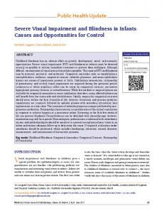
When assessing the influence of visual impairments on perceived quality, the type of video can have a significant impact [44], [45], [46]. It is generally known that, for example, the amount of motion and spatial details in a video sequence affect the visibility of visual degradations [47]. In order to quantify the spatial and temporal information of a video sequence, ITU Recommendation P.910 [44] defines two complexity measures which are calculated for each video frame at time n (Fn ). The spatial perceptual information measurement (SI) is based on a Sobel-filter and is calculated as the maximum value of the standard deviations of each Sobelfiltered frame at time n:
cheetah
15
BBB SSTB
10
rush hour
(2)
where Mn (i, j) = Fn (i, j) − Fn−1 (i, j). Since both the SI and TI values for a video sequence are represented by the maximum value over all the video frames, peaks (caused by for example scene cuts) may result in an overall SI or TI value which is not representative for a particular video sequence [48]. Results showed that the human perception of spatial and temporal information in a video sequence can be better approximated by calculating the upper quartile value instead of the maximum value. Hence, the authors in [48] propose the Q3.SI and Q3.T I perceptual information measurements. These are calculated similar to equations 1 and 2, but the third quartile value (Q3) is calculated over all the video frames instead of taking the maximum SI and TI value. In the case of subjective video quality testing, the selected test sequences should span a wide range of spatial and temporal information. Therefore, we calculated the Q3.SI and Q3.T I values for a series of test sequences available from the Consumer Digital Video Library (CDVL) [49]3 , the Technical University of Munich (TUM) and open source movies and selected eight different sequences to be used in our subjective test. All original test sequences were taken from progressively scanned content with a resolution of 1920x1080 pixels and a frame rate of 25 frames per second. Each video sequence was trimmed to a duration of exactly 10 seconds. Figure 2 shows the calculated Q3.SI and Q3.T I values for our selected sequences and a short description of each sequence is provided in Table I. Sequences marked with a star indicate that the content is taken from an open source movie. For encoding our eight selected HD sequences, we first collected realistic encoding settings by analyzing HD content from online video services and by inspecting the default settings recommended by commercially available H.264/AVC encoders. More specifically, we are interested in discovering 3 http://www.cdvl.org
ED
5 0 0
10
20
30
40
50
60
70
80
90
Q3.SI Fig. 2. Calculated Q3.SI and Q3.TI values, as suggested in [48], for our eight selected source sequences.
The temporal perceptual information (TI) is similarly calculated as SI, but is based on the pixel difference between two consecutive frames: T I = maxtime {stdspace [Mn (i, j)]},
purple4e
20
TABLE I D ESCRIPTION OF THE SELECTED TEST SEQUENCES . Sequence basketball
Source CDVL
BBB*
Big Buck Bunny
cheetah
CDVL
ED*
Elephants Dream
foxbird3e
CDVL
purple4e
CDVL
rush hour
TUM
SSTB*
Sita Sings the Blues
Description Basketball game with score. Camera pans and zooms to follow the action. Computer-Generated Imagery. Close-up of a big rabbit. Slight camera pan while following a butterfly in front to the rabbit. Cheetah walking in front of a chainlink fence. Camera pans to follow the cheetah. Computer-Generated Imagery. Fixed camera focusing on two characters. Motion in the background. Cartoon. Fox running towards a tree and falling in a hole. Fast camera pan with zoom. Spinning purple collage of objects. Many small objects moving in a circular pattern. Rush hour in Munich city. Many cars moving slowly, high depth of focus. Fixed camera. Cartoon. Close-up of two characters talking. Slight camera zoom in.
the most commonly used number of slices per picture, the Group Of Pictures (GOP) size and the number of B-pictures. We found that the video sequences are usually encoded using 1, 4 or 8 slices per picture and a GOP structure containing 0, 1 or 2 B-pictures. We also noticed that different GOP sizes are used but an average GOP size between 12 and 15 frames is typically used in an IPTV environment [50]. In this article, we are primarily interested in the influence of network impairments on perceived quality. Therefore, the encoding bit rate was set high enough in order to avoid the presence of visual coding artifacts. Based on this analysis, we used the following encoding settings: • • • • •
Number of slices: 1, 4 and 8 Number of B-pictures: 0, 1 and 2 GOP size: 15 (0 or 1 B-picture) or 16 (2 B-pictures) Closed GOP structure Bit rate: 15 Mbps
This way, each original sequence was encoded using nine different configurations giving a total number of 72 encoded sequences. We also visually inspected each encoded sequence in order to ensure the absence of any coding artifacts.
IEEE TRANSACTIONS ON BROADCASTING
5
B. Impairment generation Any H.264/AVC compliant bitstream must only contain complete slices. Even in the case when only a small portion of a slice is lost, the entire slice should be discarded. Therefore, we impaired the encoded sequences by dropping particular slices. We used Sirannon4 [51], our in-house developed open source modular multimedia streamer, in order to drop specific slices from an encoded H.264/AVC video stream according to the configuration depicted in Figure 3. In our setup, a raw H.264/AVC Annex B bitstream is first packetized into RTP packets according to RFC3984 [52]. No aggregation was used during the packetization process which implies that a single RTP packet never contains data belonging to more than one encoded picture. Next, slices are dropped by discarding all the RTP packets carrying data belonging to the same slice. After unpacketizing, the resulting impaired H.264/AVC Annex B compliant bitstream is saved to a new file.
further reduce the number of scenarios we searched for the least unique scenarios and removed them from the design. This will result in a design for which the remaining points lie as far away from each other as possible [54]. As each scenario is identified by a combination of the six parameters (6-tuple) described above, the least unique scenario is the one for which every parameter value occurs the most in the design. For example, in the following scenarios the third one is the least unique: (1, I, begin, 2, bottom, 0) (1, P, middle, 1, top, 1) (2, P, begin, 2, top, 0) Using this experimental design, 48 impairment scenarios were selected which we applied to our eight selected sequences resulting in a total number of 384 impaired video sequences. No visual impairments were injected in the first and last two seconds of video playback. Since the impaired video sequences cannot be decoded properly with the H.264/AVC reference software except in the simplest cases of loss patterns, we adjusted the JM Reference Software version 16.1 [55] to enable error concealment in case of picture drops [56]. As a concealment technique, frame copy has been implemented.
Fig. 3. RTP packets, which carry data from particular slices, are dropped using the nalu-drop classifier component. After unpacketizing, the resulting impaired sequence is saved to a new file.
C. Subjective quality assessment methodology
We are interested in investigating the visibility of losing one or more slices and one or more entire pictures. Therefore, the following parameters were used to create different impairment scenarios: • Number of B-pictures between two reference pictures (0, 1 or 2) • Type of picture in which the first loss is inserted (I, P or B) • Location within the GOP where the loss is inserted (begin, middle or end) • Number of consecutive slice drops (1, 2 or 4) • Location within the picture of the first dropped slice (top, middle or bottom) • Number of consecutive entire picture drops (0 or 1) In the case of consecutive slice drops, all dropped slices belonged to the same picture. As such, dropping two or four consecutive slices was not taken into account when the pictures were encoded using a single slice. Consecutive pictures were only dropped in sequences encoded with one slice per picture. Furthermore, we only considered dropping two consecutive P-pictures and two consecutive B-pictures. Creating a full factorial [53] of all possible combinations of the parameters for impairing the sequences would result in 486 scenarios. However, not all combinations are feasible; for example, changing the location within the picture of the first dropped slice is only meaningful when the sequence is encoded using multiple slices. Therefore, all illegal combinations were removed after generating the full factorial. To 4 Sirannon
is formerly known as xStreamer.
The different sequences were presented to the subjects based on the Single Stimulus (SS) Absolute Category Rating (ACR) assessment methodology as specified in [44]. Using this methodology implies that the video sequences are shown one at a time without the presence of an explicit reference sequence. This also corresponds with watching television, where viewers can only evaluate the received video signal [57], [58]. Prior to the start of the subjective experiment, all subjects received specific instructions on how to evaluate the different video sequences. After screening the subjects for color vision and visual acuity (using Ishihara plates and a Snellen chart, respectively), three training sequences were presented. This training session was used to get the subjects familiarized with the different kinds of impairments which could be perceived during the experiment. After watching each sequence, viewers first had to indicate whether they perceived a visual impairment. If the latter was the case, they were also asked to provide a quality score for that particular sequence using the 5-grade ACR scale depicted in Figure 4. 5 4 3 2 1
_ _ _ _ _
Imperceptible Perceptible but not annoying Slightly annoying Annoying Very annoying
Fig. 4. Five-level grading scale [44] presented to the subjects, after each sequence, for recording impairment visibility and annoyance.
In order to avoid viewer fatigue, the overall experiment duration should not exceed 30 minutes. Therefore, we created
IEEE TRANSACTIONS ON BROADCASTING
six different datasets each containing 76 sequences, which include both original encoded and impaired video sequences. As such, the duration of each dataset was limited to about 20 minutes. The order of the video sequences within a single dataset was randomized at the start of the trail so that no two subjects evaluated the sequences in exactly the same order. The video sequences were displayed on a 40 inch full HD LCD screen with subjects seated at a distance of 4 times the picture height. A total number of 40 non-expert viewers, aged between 18 and 34 years old, participated with the subjective experiment. Amongst them, 11 were female and 29 were male test subjects. Each dataset was evaluated by exactly 24 subjects. As a result, most of the subjects evaluated more than one dataset although not necessarily on the same day. We also performed a post-experiment screening of our test subjects using the methodology described in Annex V of the VQEG HDTV report [20] in order to ensure no outliers were present in our subjective data. This methodology is based on the linear Pearson correlation coefficient and rejects a subject’s quality scores in case the correlation with the average of all the other subjects’ quality ratings drops below the acceptability threshold. V. D ECISION TREE - BASED MODELING OF IMPAIRMENT VISIBILITY
In this article, we are interested in determining whether the loss of some part of the video stream will result in a visible impairment. In other words, we want to be able to classify the occurrence of packet loss as visible or invisible for the average end-user. Reibman et al. [35] and Kanumuri et al. [36] both used a decision tree classifier for modeling packet loss visibility, which we also used in our previous research [17]. A decision tree, as depicted in Figure 5, is built up using different nodes and end nodes (also known as leaves) and is traversed from top to bottom.
Fig. 5. Basic decision tree composed of different nodes and leaves which is traversed from top to bottom.
While traversing the tree, a decision on which path to follow down is made at every node based on the value of one or more of the attributes used to construct the tree. This evaluation continues until a leaf node is reached at which point the classification is completed. The label associated with this leaf node then determines, for example, error visibility. The use of a decision tree for performing classification offers several advantages. First of all, the decision tree is a white
6
box showing the complete internal structure of the classifier. This implies that an in-depth analysis can be performed which can lead to better insights and more conclusions on how the classification is performed. As the evaluation of a node in the decision tree comes down to an if-else evaluation, a decision tree can also easily be implemented. Another big advantage of decision trees is that they can handle both numerical and categorical parameters [59]. For evaluating the performance and reliability of a decision tree, the overall classification accuracy and the true positive (TP) rate can be considered. The classification accuracy is defined as the ratio between the number of correctly made classifications and the total number of classifications. In the case of classifying packet loss as visible or invisible, the TP rate for the visible packet losses represents the percentage of visible losses correctly classified as being visible. VI. R ESULTS For modeling packet loss visibility, parameters need to be extracted from the network and/or video bitstream in order to identify the location and extent of the initial loss. These parameters are then used for building different decision trees. In this section, we first provide an overview of the different parameters used for predicting impairment visibility. Next, we present different decision trees for classifying packet loss as visible of invisible to the average end-user. A. Parameter extraction As we are targeting a no-reference bitstream-based visual quality metric, only information extracted from the network and the received encoded (impaired) video stream is available for constructing our decision tree. Different parameters are extracted from the network and the video bitstream in order to identify the location of the loss and characterize the video sequence. The location of the loss is identified by the type of the lost slice, the location of this slice within the picture and the GOP, and the number of consecutive slice losses. Characterizing the pictures affected by the loss is performed by extracting information at the macroblock and the motion vector level. As such, we calculate the average motion vector lengths and standard deviations. Statistics concerning the macroblock partitions and types are also calculated. All these statistics are calculated within the GOP containing the loss. In case the loss occurs in the I picture, the statistics are calculated from the remaining B and P pictures in the GOP. When the impairment originates from a P picture, statistics are calculated from the I picture (at the beginning of the GOP) and all the other P pictures in the GOP, the B-pictures are not used in this case. Similar when a loss occurs in a B picture, only the I picture and the other B-pictures in the GOP are taken into account when calculating the statistics. An overview of all extracted parameters is listed in Table II. B. Modeling packet loss visibility For constructing different decision trees, we used the Waikato Environment for Knowledge Analysis (WEKA) [60],
IEEE TRANSACTIONS ON BROADCASTING
VIDEO BITSTREAM IN ORDER TO IDENTIFY THE LOCATION OF THE LOSS AND CHARACTERIZE THE VIDEO SEQUENCE .
Parameter b pics, nb slices, gop size
contentclass imp pic type, perc pic lost
imp in gop pos, imp in pic pos
imp imp imp drift perc perc perc perc perc perc perc
cons slice drops, cons b slice drops, pic drops pb 4x4, perc pb 8x8, pb 16x16, pb 8x16, pb 16x8, perc i 4x4, i 8x8, perc i 16x16 i mb, perc skip, ipcm
I perc 4x4, I perc 8x8, I perc 16x16 abs avg coeff, avg qp
I abs avg coeff, I avg qp
perc zero coeff, I perc zero coeff
avg mv x, avg mv y, stdev mv x, stdev mv y
avg mv xy, stdev mv xy
perc zero mv
Description Number of B-pictures, slices per picture and GOP size as specified during encoding. Sequence content classification (see Table IV). Type (I, P or B) and percentage of slices lost of the picture where the loss originates. Temporal location within the GOP (begin, middle, end) and spatial location within the picture (top, bottom, middle) of the first lost slice. Number of consecutive slice drops, number of consecutive B-slice drops and number of entire picture drops. Temporal duration of the loss. Percentage of I, P & B macroblocks of type 4x4, 8x8, 16x16, 8x16 and 16x8, averaged over the pictures in the GOP containing the loss.
indicate whether they perceived a visual impairment or not. Based on these results, we classify packet loss to be visible when 75% or more of the subjects perceived the impairment. Otherwise, the impairment is classified as invisible. When plotting the Mean Opinion Score (MOS) of each sequence against the percentage of the subjects who perceived an impairment in the corresponding sequence, as depicted in Figure 6, we also noticed that the MOS drops below 4 starting from a detection threshold of 75%. 5
4
3
MOS
TABLE II OVERVIEW OF ALL PARAMETERS EXTRACTED FROM THE RECEIVED
7
2
1
0 0
Percentage of macroblocks encoded as I, skip and PCM, averaged over the pictures in the GOP containing the loss. Percentage of macroblocks of type 4x4, 8x8 and 16x16 in the first I or IDR picture of the GOP containing the loss. Absolute average value of the macroblock coefficients and QP value, averaged over the P or B pictures in the GOP containing the loss. Absolute average value of the macroblock coefficients and QP value in the first I or IDR picture of the GOP containing the loss. Percentage of zero coefficients, averaged over the P or B pictures in the GOP containing the loss and average of zero coefficients in the first I or IDR picture of the GOP containing the loss. Average absolute motion vector length and standard deviation in x- and ydirection, averaged over the P or B pictures in the GOP containing the loss. Motion vector magnitudes have quarter pixel precision. Average and standard deviation of the sum of the motion vector magnitudes in x- and y-direction, averaged over the P or B pictures in the GOP containing the loss. Motion vector magnitudes have quarter pixel precision. Average percentage of zero motion vectors, calculated over the P or B pictures in the GOP containing the loss.
an open source data mining software package. As our total number of sequences is limited to 384, we used 10-fold cross validation for constructing and validating the built trees. During k-fold cross validation, the entire dataset is split into k subsets of which k − 1 are used for building the tree and one dataset is used for validating the tree. This process is repeated exactly k times, each time selecting a different subset for validation. A common value used for k is 10, which minimizes the variance over the different runs [61]. During the subjective experiment, subjects were required to
10
20
30
40
50
60
70
80
90
100
% Perceived Fig. 6. Percentage of the viewers who perceived the impairment versus the MOS of the corresponding sequence.
As such, we classify packet loss visibility based on a single threshold as opposed to the two thresholds (75% and 25%) used by Reibman [35] and Kanumuri [36] as explained in section III. Our previous research [17] showed that the classification accuracy can be improved when considering the two thresholds mentioned above. However, the drawback of this approach is that not all packet losses can be classified, i.e. packet losses which have a detection threshold between 25% and 75%. By using a single detection threshold, we ensure that all losses will be classified as visible or invisible. In our previous research [17], we used high-level information extracted from the bitstream for modeling packet loss visibility without the need for parsing the video data. Our results showed that the obtained decision trees had a high accuracy taking into account that only a limited amount of parameters were used during the modeling process. Using the data obtained in this article, we start off by modeling a decision tree using the following high level parameters: imp_pic_type, imp_in_gop_pos, imp_in_pic_pos, imp_cons_slice_drops, imp_cons_b_slice_drops, perc_pic_lost, imp_drop_next_pic. The resulting tree, depicted in Figure 7a, shows that only five parameters are needed to classify packet loss visibility. Looking at the tree into more detail, we see that a loss of up to two B-pictures is not perceivable and that losses in Ipictures are always perceived, even if only one out of eight slices is lost. In case the loss originates from a P-picture, error visibility depends on the percentage of the slices lost and the location of the P-picture within the GOP. To be more precise, when only a small portion of the slices is lost, the impairment is not perceived. When more than 25% of the slices in the picture is lost, impairment visibility is determined by the
IEEE TRANSACTIONS ON BROADCASTING
8
TABLE III C ALCULATED AVERAGE DRIFT ( TEMPORAL EXTENT ) AND STANDARD DEVIATIONS OF IMPAIRMENTS ORIGINATING FROM PACKET LOSS IN
P- PICTURES , DEPENDING ON THE LOCATION WITHIN THE GOP OF THE FIRST AFFECTED P- PICTURE .
avg(drift) stdev(drift)
(a)
Location within GOP BEGIN MIDDLE END 14 9 4 1 2 2
spectively 84.0% and 82.1%. Taking into account that only a limited number of high-level parameters are used, packet loss visibility can be predicted with a high accuracy. Results in [17] and [41] show that the prediction accuracy can be increased when taking into account the video content and characteristics. Therefore, we clustered our eight sequences (cfr. Figure 2) into four different content classes as shown in Table IV and make this additional parameter (’contentclass’) available to the modeling process. TABLE IV C LUSTERING OF THE DIFFERENT VIDEO SEQUENCES , BASED ON THE AMOUNT OF MOTION AND SPATIAL DETAILS , INTO FOUR CONTENT CLASSES . Content class A B C D
(b) Fig. 7. Decision trees for classifying the occurrence of packet loss as visible or invisible to the average end-users, using only high level parameters extracted solely from the received encoded video bitstream (a) and with additional content classification (b).
temporal extent of the error (drift). As such, impairments are not visible in case the packet loss affects a P-picture located at the end of the GOP which results in a short drift of the error. Table III shows the average drift caused by losses in Ppictures, depending on the location of that picture within the GOP. In our experimental design, we dropped up to four slices in our sequences encoded with eight slices. As such, the branch imp_cons_slice_drops > 2 implies that the errors are always perceived when 50% of a P- or I-picture is lost in these sequences. Our data analysis showed that impairments are not always perceived when 50% of a picture, encoded with four slices, is lost. Hence, a lower number of slices per picture might be preferred as this appears to be better in terms of error visibility. The overall classification accuracy of this tree equals 83.1%. The TP rates for visible and invisible impairments are re-
Characteristics low motion, low spatial details high motion, medium spatial details high motion, high spatial details low motion, high spatial details
Sequences BBB, rush hour cheetah, foxbird3e basketball, purple4e ED, SSTB
As can be seen in Figure 7b, including the content classification increases the overall complexity of the tree in terms of tree size. However, still only five parameters are used throughout the entire tree. Similar to the previous tree, losses in B-pictures are never detected, independent of the type of video. According to the tree, content classification becomes an important factor in case packet loss occurs in I- or P-pictures. Perceptibility of impairments originating in I-pictures depends on the number of slices lost. During our impairment generation, we dropped 25%, 50% or 100% of the slices belonging to a particular picture. As such, the branch corresponding with perc_pic_lost > 0.5 implies that an entire I-picture is lost. At this point, our error concealment comes into play and shows that impairments can be masked in sequences with low amounts of motion (content class D). The fact that packet loss impairments are less visible in video sequences with still camera motion also corresponds with the research findings of Reibman et al. [40]. From Figure 2 it can be seen that the amount of motion in the rush hour sequence corresponds with the sequences of content class D. According to the tree, losing an entire I-picture in content class A sequences results in a visible impairment. However, inspecting the classification accuracy of that branch revealed that only 50% of the predictions is correct. The data analysis showed that loosing an entire I-picture in the rush hour sequence is never perceived whereas the loss is perceived in case it occurs in the BBB sequence. This indicates that
IEEE TRANSACTIONS ON BROADCASTING
it might be better to drop an entire I-picture (even if only a limited number of slices is lost) in low motion sequences and use the concealment at the decoder to mask the error. In our case, low motion sequences are characterized by a Q3.T I value ≤ 13. Losses originating from P-pictures are not perceivable in case only a small portion of the picture is lost. As was the case in our previous tree, the branch imp_cons_slice_drops > 2 again only applies to the sequences encoded with eight slices per picture. Again, losing 50% of the slices in our sequences encoded with eight slices per picture results in a visible impairment. The path imp_cons_slice_drops 1 refers to losses of half a picture or losing two consecutive B-pictures. In that case, impairment visibility is content dependent and more clearly visible in high motion areas. Content is identified based on the distribution of the macroblocks and the average length of the motion vectors. As mentioned in section VI-A, these parameters are calculated only using the information available in the correctly received B-pictures of the current GOP. The amounts of motion and spatial details are also important factors when more than 25% of a P-picture is lost. According to the tree, impairments are again easier detected in areas with high motion, corresponding with our previous trees and our previous research [17]. The classification avg_mv_xy 2), similar to our previous tree. When losing two out of four slices or two consecutive Ppictures, impairment visibility is dependent on the amount of spatial information. The parameter perc_pb_16x16 refers to the average percentage of inter coded 16x16 macroblock partitions in the correctly received P-pictures of the current GOP. The split perc_pb_16x16