congested urban road networks. Phenomena such as the formation and dispersion of queues are relevant and cannot be reproduced by traditional static models ...
MATHEMATICAL AND COMPUTER MODELLING
PERGAMON
Mathematical and Computer Modelling 35 (2002) 643-656 www.elsevier.com/locate/mcm
N o d e and Link M o d e l s for N e t w o r k Traffic F l o w S i m u l a t i o n V. ASTARITA Dipartimento di Pianificazione Territoriale University of Calabria Arcavacata di Rende (CS), Italy vastarit©unina, it
A b s t r a c t - - I n this paper, after introducing a classification of dynamic network loading (DNL) procedures (based on time, space, and demand discretization), many new methodologies recently presented are discussed. Some analytical properties of the point packet approach, recently studied by Chabini and Kachani [1], using generalized Dirac functions, are discussed, and results are extrapolated to the proposed procedure (called MICE [2]). The connection between the dynamic network loading procedure MICE and the analytical formulation presented in [3] is explained. The same demand discretization is suggested in the solution of all analytical traffic flow models. (~) 2002 Elsevier Science Ltd. All rights reserved.
Keywords--Traffic flow, Trafficsimulation. 1. I N T R O D U C T I O N The classical network models of transportation systems are based on the assumptions of stationarity. This assumption, which is acceptable for many applications (i.e., city planning), does not allow us to simulate satisfactorily certain types of transportation systems such as heavily congested urban road networks. Phenomena such as the formation and dispersion of queues are relevant and cannot be reproduced by traditional static models (see [4-6] for a good introduction to the problem). Traffic engineer scientists have been studying for years the modelling of the dynamic behaviour of many of the components of a transportation system, but only recently the research efforts in traffic modeling and traffic assignment have been focused on the modelling of traffic dynamic behaviour in a complete network system. A large number of models and procedures have been proposed that are usually referred to, in the literature, as (within-day) dynamic traffic assignment (DTA) models. These models can be used both to evaluate traffic flows and, what is more relevant, to simulate the effects of regulation strategies on users' behaviour. These models originate from static network traffic assignment models based on stochastic or deterministic user equilibrium. In many early cases, dynamic traffic assignment models were merely an extension of the concepts contained in static models. But the extension of within-day static models to take into account within-day dynamics is by no means straightforward, since within-day dynamic supply modeling requires completely new definitions and formulation of the problem [7]. In order to perform DTA, in fact, it is necessary Research supported by the Italian M.U.R.S.T. 0895-7177/02/$ - see front matter (~) 2002 Elsevier Science Ltd. All rights reserved. PII: S0895-7177(01)00187-X
Typeset by A.h/cS-TEX
644
V. ASTARITA
to solve the dynamic network loading problem (DNL) that has been indicated (by the specialists of static traffic assignment) as the reproduction of within-day variable link performances given a corresponding O/D demand and users'choice model. The dynamic network loading problem, in other words, is the reproduction of the traffic flow motion on the network. It has to be studied with time advancing mathematical models that are commonly referred (by traffic engineering specialists) as traffic simulation models. The DNL problem, so far, has been studied with a great number of different approaches that are sometimes indicated as: • microsimulation models [8-11]; • mesosimulation models: heuristic generalization of within-day static methods [12,13]; exitfunction methods [14-20]; packet-approaches and simulation procedures [2,21-31]; continuous time link models [32-36], where often the problem of finding conditions for the respect of FIFO on a link is discussed; • macrosimulation models (continuous in time and space flow models [37-42]). The above-mentioned types of DNL are not so dissimilar from each other: there is a continuous spread among the conceivable network franc simulation models. Due to a different discretization of time, space, and demand, sometimes different simulation procedures are not recognized as being originated by the same underlying model (very interesting the case in [39,41,42]). Sometimes the confusion arises also because a distinct discretization of the same model can lead to quite different results. Moreover, two important problems are still open in traffic network simulation: • a bad representation of traffic dynamics: some of the proposed models do not even address the significant problem of the backward propagation of congestion; • the difficulty of collecting experimental data to test (and sometimes even to run) the models. Both problems are far from being solved, and many researchers are concentrating their efforts on this topic (DNL) that has so many practical applications. The model proposed in this paper has some advantages and also many disadvantages compared to other approaches. The model is discussed in the following not because it is better than other approaches, but because it is used as a starting point to clarify that some common problems, the backward propagation of congestion at the intersection level, can be solved by using packets to represent traffic vehicles. In fact, the model is a time-advancing algorithm that follows explicitly the motion of packets on the network, but can be seen also as a discrete solution of a time advancing continuous analytical differential equation system. The model is based on the analytical DNL model presented in [3], which is able to deal with the spill-back of congestion and is based on the preceding link model formulation presented in [19,32,33,35,36]. This paper is organized as follows: in Section 2, a classification of dynamic network loading (DNL) procedures (based on time, space, and demand discretization) is introduced. Many problems that arise in DNL models are discussed in Section 3. In Section 4, some general definitions are introduced. In Section 5, the proposed model is briefly discussed, and at last in Section 6 some analytical properties of the point packet approach are discussed and results are extrapolated from the proposed procedure (called MICE [2]) to other analytical models.
2. TIME, SPACE, A N D D E M A N D DISCRETIZATION As pointed out in the introduction, a great number of different DNL approaches have been presented and, due to the continuous spread among the conceivable network traffic simulation models, many others still are conceived every year. In the following, a classification based on the discretization adopted by several models is proposed even if some approaches consist of "mixed" modelling so that differences are not so considerable as to allow a definite grouping. Moreover, it is quite hard to state that all the same
Network Traffic Flow Simulation
645
requirements are respected by a group of similar models, since very similar models may not respect the same requirements. The following main modelling approaches can be identified: (1) (2) (3) (4) (5)
microsimulation models, continuous in time link models, discrete in time link models, models following a packet approach, and macrosimulation models (continuous in time and space models).
According to time, space, and demand discretization, it is possible to represent models in a three-dimensional space where the x, y, and z axes are time, space, and demand. The 0 value would be representative of a continuous model, and a finite value would represent a finite step for the representation of time, space, or demand. A continuous in-time model will be located on the space-demand plane (y-z). In Figure 1, examples of the above-mentioned models are located by four points and a plane. Microsimulation models are based on the simulation of the movement of single users. Microscopic simulation is indicated in reproducing some specific local traffic situations, such as intersection and parking facilities, or for the evaluation of control strategies which act on single individual driver behaviour. Some mixed models have been proposed, based on a microscopic or quasi-microscopic simulations, obtaining macroscopic link characteristics such as speed and density [28].
Demand
Micro-simulation models (1) . - "
e
~ " .
models (5)
~ n u o u s
Discrete in t i m e link m o d e l s (3) O
in t i m e link m o d e l s (2)
Space
Figure 1. Three-dimensional representation of network traffic models according to time, space, and demand discretization.
Many authors (Friesz et al. [18], Wie et al. [20], Boyce et al. [151, Fernandez and De Cea [431, and Adamo et al. [3]) have proposed formulations of continuous in time link models that are based on a space discretization which divides up the path of the users into links which together form the network. Some of these continuous models have been numerically solved with a time discretization and so can be related to concepts originated in the discrete in time link model proposed by Merchant and Nemhauser [14]. Discrete in time link models are based on the two following equations: x, u, and w are defined in the following, respectively, as number of vehicles
646
v. ASTARITA
on a link, entering and exiting flows; i and j are, respectively, time interval and link number:
(1) (2)
Xi+l,j = xi,j + ui,j -- wi,j, =
w (xia)
.
In packet approach methods, users are grouped together to form packets that can be moved along the network so to realize a discretization of the demand of each OD couple. It is possible to distinguish between a point packet approach [2,27,31] in which a group of users is concentrated into a single point and a continuous packet approach [23-25,29], where the users are supposed uniformly distributed in time or space along the packet between the packet edges. This approach can rely on a link modelling which facilitates the computation and can respect all the requirements described in this paper. Other mesosimulation models include [44], where a traffic assignment model with distributed parameters is proposed in the context of system optimal conditions with particular attention to FIFO rule respect. Continuous in time and space models (or macroscopic models) are more sophisticated models that are based on continuous traffic simulation such as in the Lighthill and Whitham's model [38] or Payne's model [45]. In macroscopic DNL models, vehicles are modelled with piecewise continuous functions of density and flow, in space-time, analogous to fluid flow. The mathematical theory behind these models is based on temporal, one-dimensional fluid dynamics. Conservation laws are respected. The state variable(s), density (and sometimes speed), is described over the entire length of each link. Flow and speed are functions of the state variable(s). Also, macroscopic models assume homogeneous traffic characteristics and sometime deterministic modelling relationships. The simplest macroscopic traffic models are based on the concept that vehicle traffic at a given point in space-time is affected only by local traffic within a neighbourhood of that point [5]. Flow and density are related by empirical measurements [46]. Their limits consist of their applicability, arising from the complex numerical solution. Many models of this type have been developed for freeway network simulation [40,47]. The cell transmission models of Daganzo [5] originate from the Lighthill and Whitham's model [38], as shown in Figure 2.
Demand
~
_Lightill and Whitham model
/J "--Time
"-., 1
Cell transmission model
nsion dx
Space
Figure 2. The Daganzo cell transmission model [5] originates from the Lighthilland Whitham's model.
The following two simple categories can be defined for DNL methods and are quite different in demand (traffic flow) discretization. •
Time-advancing differential equation systems that represent the motion of traffic as being the motion of a fluid. These equations have the same numerical problems as nonstationary fluid dynamics equations. In these models, the traffic being a continuous fluid, the FIFO
Network Traffic Flow Simulation
647
rule has to be respected, but in practice when the models are discretized, for solution, it is very difficult to maintain a complete respect of FIFO rule. These models can be represented as being on the time-space plane as in Figure 3. * Time-advancing algorithms that follow explicitly the motion of vehicles on the network. Sometimes vehicles are grouped into packets. These models can be represented, in Figure 3, as all the points over the time-space plane.
Demand Planeof all the modelsbaSe:u:~on
~'Tme
.
.
.
.
.-
Spa2
Figure 3. Models based on time advancing differential equation systems.
3. T R A F F I C FLOW ARE DIFFICULT
FEATURES THAT TO REPRODUCE
The main problem with DNL approaches is the bad representation of traffic dynamics, which is caused by the difficulties in reproducing traffic flow. Traffic flow analysis is complicated both by the human factor present in drivers' behaviour and because it has some peculiar aspects unusual to other fluids (some are discussed in the following). Moreover, the complication of collecting experimental data (even only aggregated), to test the models, is the cause for so many unrealistic approaches not being rejected. Traffic flow models are different in dealing with some traffic flow aspects. In this section, the following problems are discussed and some recommendations are given for good modelling techniques: • the representation of bottlenecks and connected flow capacities and storage capacities, • traffic waves, and • intersection modelling. The spill-back of congestion on a network is the propagation of congestion backwards from a link to its upstream links. It occurs whenever a bottleneck causes a downstream queue to be so large that it impedes the incoming speed and flow of vehicles. This very common situation in many urban networks is usually caused by recurrent congestion on a day-to-day basis and is not always well represented by DNL models• In all analytical approaches to DNL, road bottlenecks can be reproduced at least at the end of links where a downstream capacity is imposed to flows exiting from each link. But a great number of microsimulation models do not have explicit capacity constraints. The idea is that the mechanism that reproduces the movement of vehicles through lane-changing and car-following rules will give as a result an intrinsic capacity constraint. Road capacities can be easily measured on the field or inferred from analogue situations, but in most microsimulation models, capacities are the outcome of not less than ten different (on average) parameters. Some of these parameters are related to the behaviour of different types of drivers,
648
V. ASTARITA
some are related to the local characteristics of the road, but usually there is no clear relation with the obtained final implicit capacity value or with the factors identified by the HCM as being related with capacity. This is perhaps the biggest pitfall of most microsimulation packages and is based on the assumption that the performance of the optimized parameters set obtained with calibration provides an approximation of the potential performance of this set in the future. The calibration of many of these models can be performed only by research institutes and so, as a result, most of the microsimulation models that are used in common practice are similar to many calibrated stock trading systems: they work only with data of the past! Among the others, one remarkable exception is the work of Van Aerde with INTEGRATION where explicit capacities can be imposed in a microsimulation model [11]. But also the representation of a network with only downstream capacities for the links is too approximate and may not be representative of real situations. In many DNL models, there has never been an attempt to give a limit to the flows entering the links through an inflow capacity and a storage capacity. The resulting flow obtained with these models may exhibit links filled with enormous numbers of vehicles, indicating that these models are essentially unqualified for practical application. Relying on common physical experience, the flow entering a link is not only limited by the upstream capacity, but when the link is full (all the space is occupied by vehicles waiting to exit), the entering flow should be smaller than or equal to the exiting flow. And this should be reflected in a dynamic network assignment model. Then two simple concepts must be taken into consideration by DNL models: • the spill-back of queues is caused by limited upstream capacity and/or link storage space; • the surplus of flow that cannot be received by a saturated link is accumulated on the preceding links. So concluding, to well represent traffic, all network models should have explicitly associated with every link a at least: • upstream capacities, Cian, • downstream capacities, C °ut, and • link storage space, C~s. The conditions of traffic in one point of the road are originated by the conditions at preceding instants of time in points situated downstream and upstream. The propagation of a traffic flow condition is usually called traffic wave. The representation of traffic waves in network traffic models is necessary. An example: the spill-back of congestion on a network is in fact the linear back-propagation of one or more congestion waves. Only analytical continuous models are able to deal well with traffic waves. But the numerical solution of many of these models faces many practical difficulties that arise from the numerical discontinuities of traffic flow parameters on the two sides of the waves. Some micro and mesosimulation models, but not many, are also able to propagate waves in both directions as a consequence of microrules for car-following. Correct traffic simulation procedures models should be able to propagate waves in both directions as explained also by Daganzo [6]. Traffic intersections have to be represented allowing congestion and queues to propagate backwards. An attempt to identify some of the problems related to intersections and queue propagation can be found in [4]. The problem is to distribute the limited resource of flow capacity on the downstream links of a node to its upstream links. The intersection representation also needs to take into account the gap acceptance phenomenon. Microsimulation models are good in achieving this target. In fact, an analytical representation of intersections that is really complete has still to be proposed. In [48], the following sentence is stated: "to be useful, analytic modellers must incorporate all meaningful physical and behavioural considerations. To do less, would be to yield the problem of traffic dynamics to simulation specialists, leaving no plausible mathematical constructs to use
Network Traffic Flow Simulation
649
in addressing the fundamental questions of existence, stability, controllability, and complexity." But it is the opinion of the author t h a t to obtain a reliable simulation of traffic flow on a network (for its intrinsic complexity), it is necessary to use some finite numerical methods or simulation techniques. Traffic specialists should address their efforts through simulation techniques t h a t at least reproduce the main features of the physical phenomenon. The difficulties of dealing with both microscopical phenomena (as gap acceptance) and macrosopical traffic behaviour (as capacities) can be solved with hybrid approaches: microsimulation models such as I N T E G R A T I O N based also on analytical considerations and/or, on the other side, macrosimulation or mesosimulation models that are solved tracking the explicit movement of vehicles on the network. These hybrid models have the potential to reproduce much better traffic flow than other approaches because they are able to reproduce both micro and macro characteristics of the traffic flow fluid. The main idea of this paper is the suggestion to reconsider micro and mesosimulation models introducing analytical relationships among aggregated traffic flow variables or alternatively (but this is only a formal difference), to solve analytical models with a demand discretization t h a t will turn these analytical models into micro or mesosimulation procedures.
4. D E F I N I T I O N S F O R T H E G E N E R A L DYNAMIC NETWORK LOADING PROBLEM T h e dynamic network loading problem can be generally stated mathematically as follows. On a t r a n s p o r t a t i o n network f~ = (N, A) composed of a set of nodes i, i E N and a set of directed arcs (links) a, a ¢ A. Traffic originates at nodes o, o E O, o C N and is destined to nodes d, dED, DcN. We have: origin-destination (o-d) pairs designated as: r, r E R C 0 x D; • a set of paths k, k E KT, t h a t connects o-d pairs r; • DT(t) as the time varying demand flow rate t h a t uses these paths, traffic departs from origins in the interval [0, T] and all traffic arrives at destination within the interval [0, T'], •
(T' > T); • the sets of arcs A + and A~- which are, respectively, the forward and backward stars of node i. The rules t h a t determine the flow of traffic on the network are different in each traffic model, but some general variables, t h a t are related to the traffic motion, can be defined in all the proposed models and are described in this section. Traffic flow introduced in the models t h a t apply a ttuidodynamic analogy in the representation of traffic is defined as the flow q(t) through a point section S of the road,
qs(t) = lim
z~t--0
N. of veh. passed through S during [t, t + At] At
(3)
This definition can be held also in models that follow explicitly the motion of vehicles on the network as microsimulation and mesosimulation models. From that definition, it is useful to indicate the flow at the first (entrance) and last section (exit) of every link a (time varying inflow rates and outflow rates) for o-d pair r, as: Ura(t) and w~(t), respectively, at time t. The number of vehicles for o-d pair r on link a at time t can be indicated as
x~(t).
(4)
We have t h a t the total inflow rates, outflow rates, and vehicles at time t on link a can be defined as
..(t)
(5)
=
r
wo(t) =
(6) r
V . ASTARITA
650
and
xo(t) = ~
x:(t),
(7)
r
respectively. ua(t), wa(t), and Xa(t) are functions of time and are related by the link flow conservation equation dxa(t) = ua(t) - wa(t). (8) dt Ura(t), Wra(t), and Xra(t) also are related by a link o-d pair flow conservation equation
dxr(t) = Ura(t) -- Wra(t). dt
(9)
The principle contained in equations (8) and (9) is valid also in microsimulation and mesosimulation models but, in this case, because u~ (t), war(t), u~ (t), and w~ (t) are not necessarily continuous, the following integral equations replace (8) and (9):
xa(t) = • X(t) =
f f
(ua(t) - wa(t)) dt,
(10)
(u~(t) - w~(t)) at.
(11)
A travel time on link a at time t (the travel time of the traffic particle that enters the link at time t) denoted as ~o(t) (12) can also be defined in every model. It is possible also to identify local variables that are useful in space continuous models. The density p (also know as concentration) between time t and time t + At at location x is the average number of vehicles on a slice of road divided by its length
E dt/At p(x,t),,~= n dx '
(13)
where ~-~ndt is the sum of the times of the n vehicles to cross the slice of road. The space-mean speed v is the average vehicle speed weighted according to the time for each vehicle to cross the slice of road, which is equivalent to the ratio of flow to density /7, • d x
v-
•dt"
(14)
n
If equations (3), (13), and (14) are defined, on the same slice of r o a d and time interval, the fundamental speed-flow-density relationship is obtained, q = vp,
(15)
which can be used to obtain the value of the third parameter given the values of the other two parameters. It is possible also to identify a local conservation equation that is equivalent to (8) with continuous space and can be obtained from (8) if the length of the link goes to 0,
Op(x, t)
----&---
+
Oq(x, t) o~
= 0.
(16)
Network Traffic Flow Simulation
651
5. T H E A N A L Y T I C A L F O R M U L A T I O N OF T H E P R O P O S E D M O D E L A simple link modelling approach has been developed in [33]. It is essentially the same as that presented in [19] and in [35], and consists (for a single destination) of the following system (17) of differential equations that constitutes a complete link model:
{
@ t t) -- u ( t ) - w(t),
T(t) = T(x(t)),
proposed model
(17)
~(t + r(t)) =
~(t)
1 + dr(t)/dt'
where each link has the following characteristics at time t: upstream flow u(t), downstream flow w(t), and a total number of users x(t) on the link, where x(t), u(t), and w(t) are continuous functions of time and r(t) is the travel time at time t (travel time of the particle that enters the link at time t). This simple model has been studied to establish the FIFO conditions and the field of applicability also for u(t) not continuous: • Lipschitz continuous functions have been investigated in [34] and in [36]; • Dirac functions have been studied in [1]. The FIFO condition can be stated formally as
t' + r (t') < t" + r (t"),
vt' < t",
(18)
which is equivalent to
W(t) = U(t + 7(t)),
(19)
where U(t) and W(t) are, respectively, the total number of vehicles entered (exited) at time t
u(t) = ~0 t u(~) d~,
(20)
/o'
(21)
w(t) =
w(~) d~.
From the results presented in [1], it is clear that the model can always be applied if FIFO violations are accepted. In this case, the third equation in (17) (equivalent to FIFO rule) has to be changed in ¢ *
w(t) = /
Jw e{zlz+r(z)